Explicit Characterization of Performance of a Class of Networked Linear Control Systems
Hossein K. Mousavi, Nader Motee

TL;DR
This paper provides a unified framework to analyze the steady-state variance performance of networked linear control systems, linking it to Laplacian eigenvalues and offering insights into connectivity thresholds and scalability.
Contribution
It introduces a general method to characterize network performance via Laplacian eigenvalues, extending previous results to arbitrary nodal dynamics and observer-based feedback.
Findings
Performance expressed as sum over Laplacian eigenvalues
Derived bounds and scaling laws for network performance
Extended methodology to observer-based and composite networks
Abstract
We show that the steady-state variance as a performance measure for a class of networked linear control systems is expressible as the summation of a rational function over the Laplacian eigenvalues of the network graph. Moreover, we characterize the role of connectivity thresholds for the feedback (and observer) gain design of these networks. We use our framework to derive bounds and scaling laws for the performance of the dynamical network. Our approach generalizes and unifies the previous results on the performance measure of these networks for the case of arbitrary nodal dynamics. We bring extensions of our methodology for the case of decentralized observer-based output feedback as well as a class of composite networks. Numerous examples support our theoretical contributions.
Click any figure to enlarge with its caption.
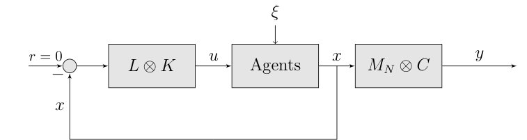 Figure 1
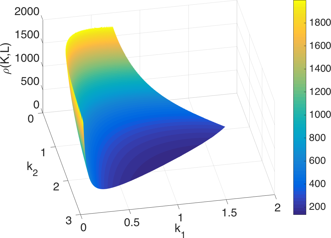 Figure 2
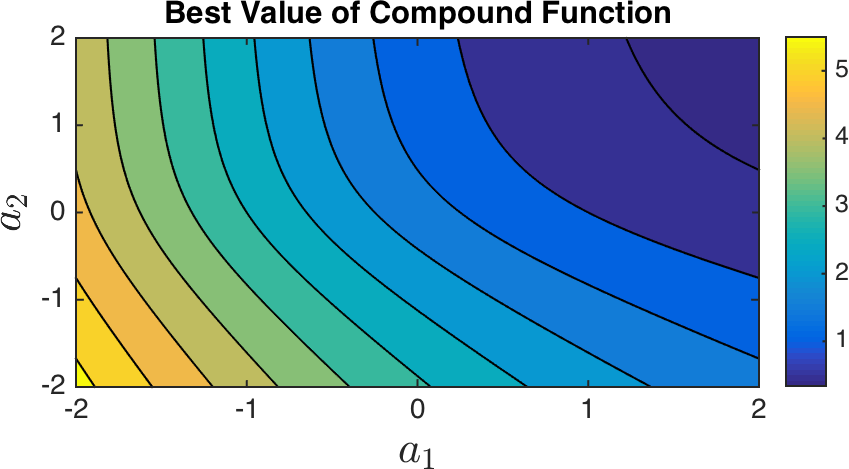 Figure 3
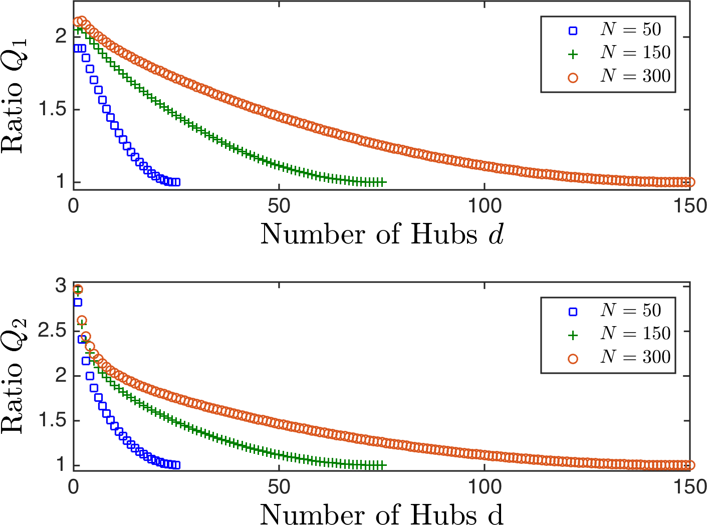 Figure 4
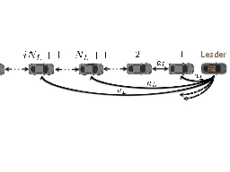 Figure 5
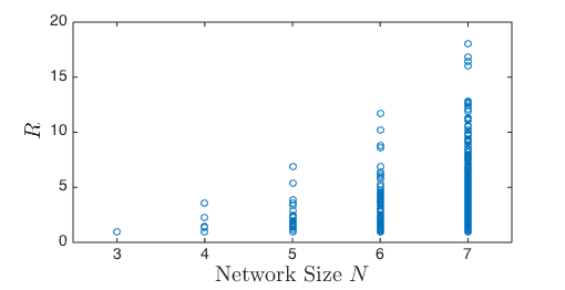 Figure 6
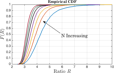 Figure 7
 Figure 8
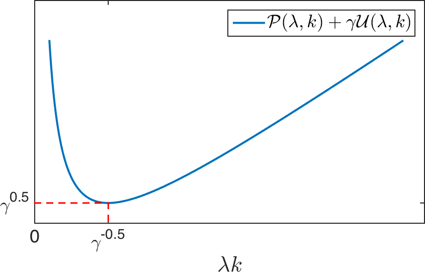 Figure 9
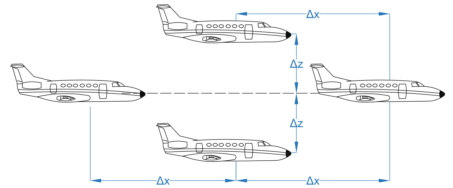 Figure 10
 Figure 11
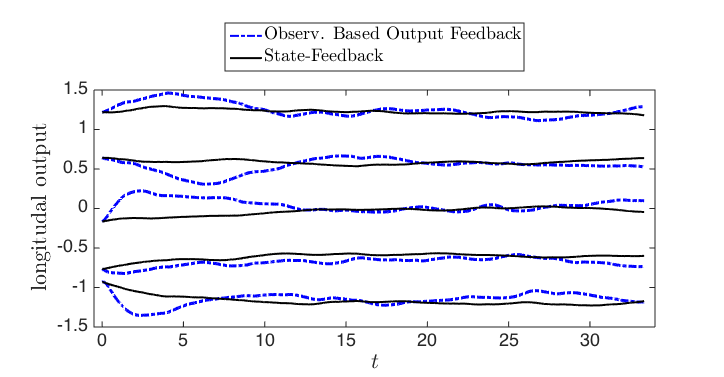 Figure 12
 Figure 13
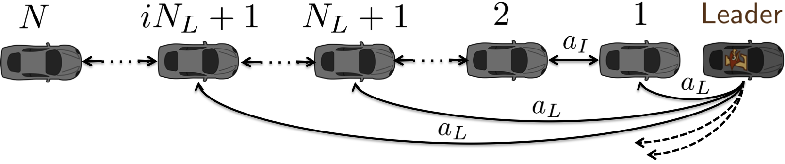 Figure 14
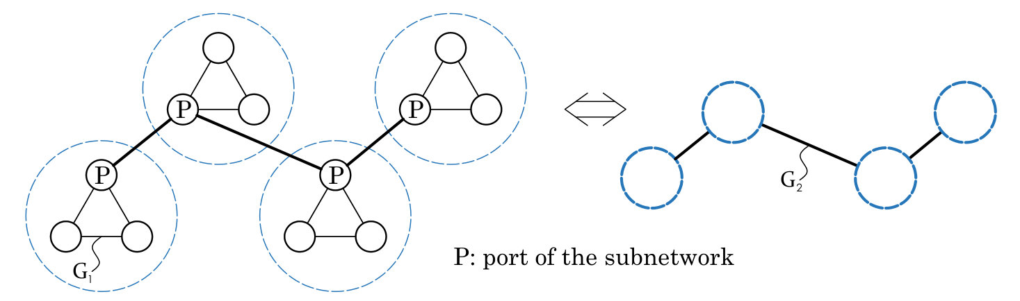 Figure 15
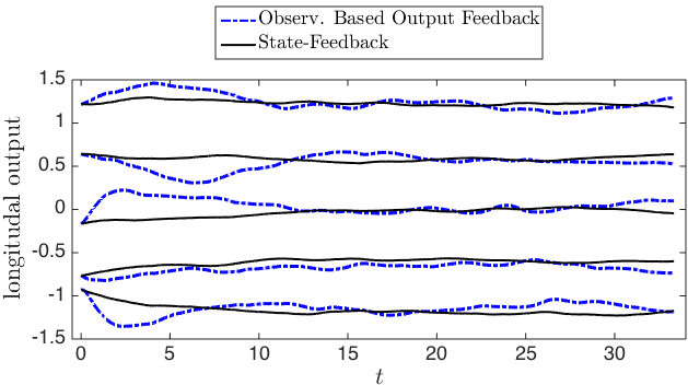 Figure 16
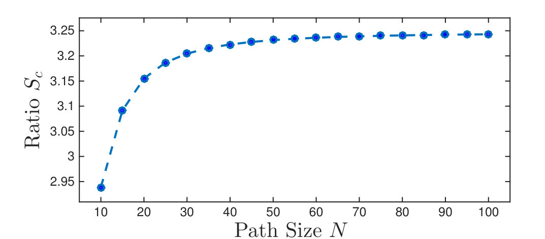 Figure 17
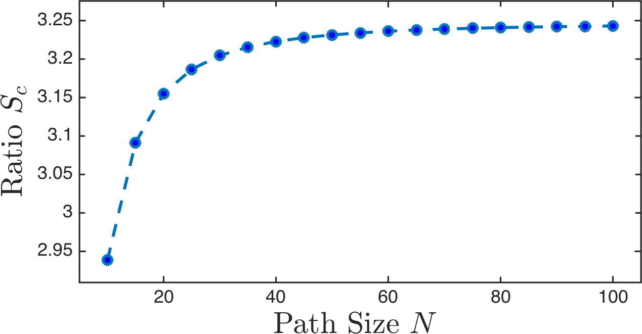 Figure 18
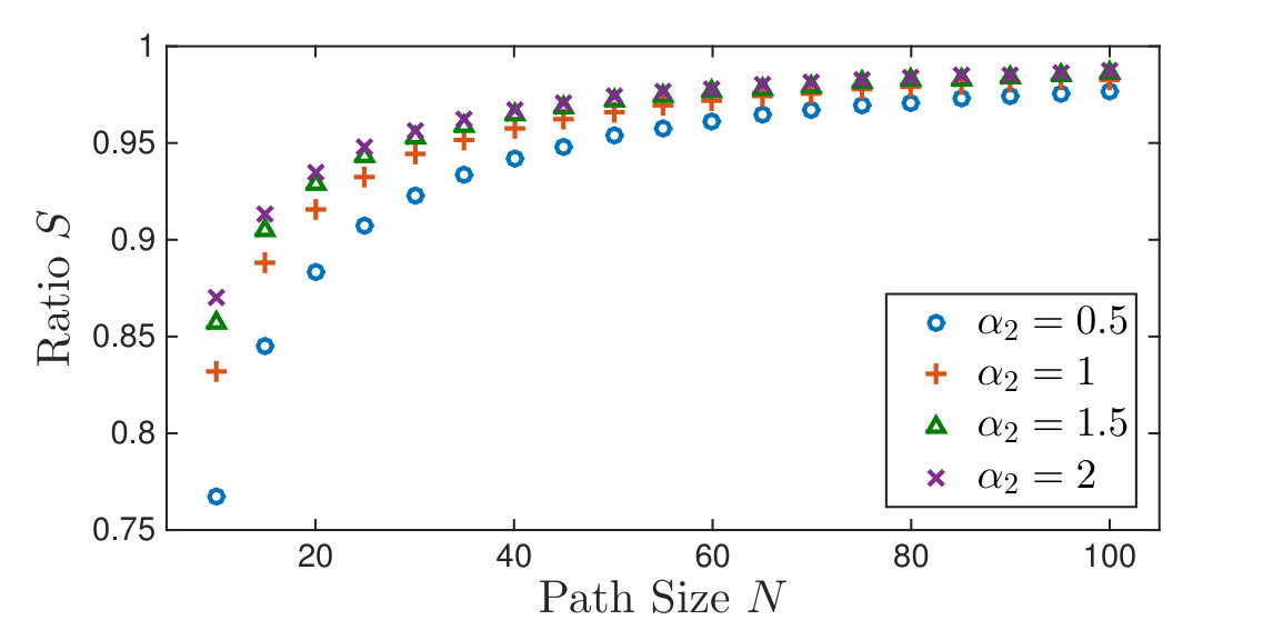 Figure 19
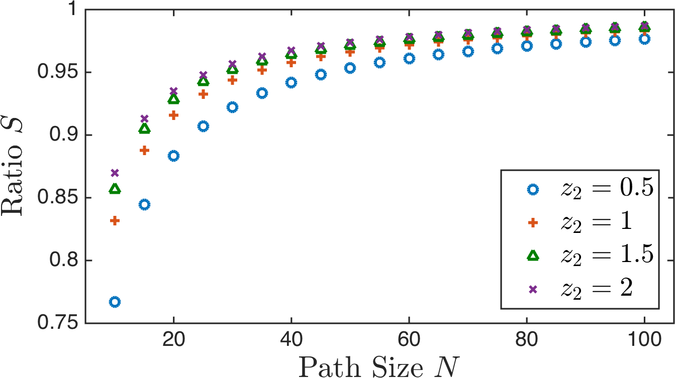 Figure 20
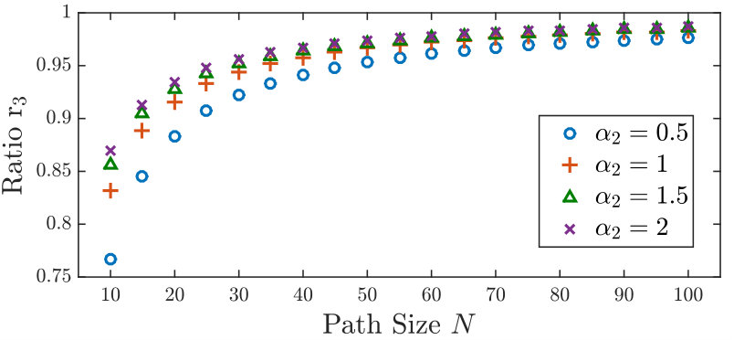 Figure 21
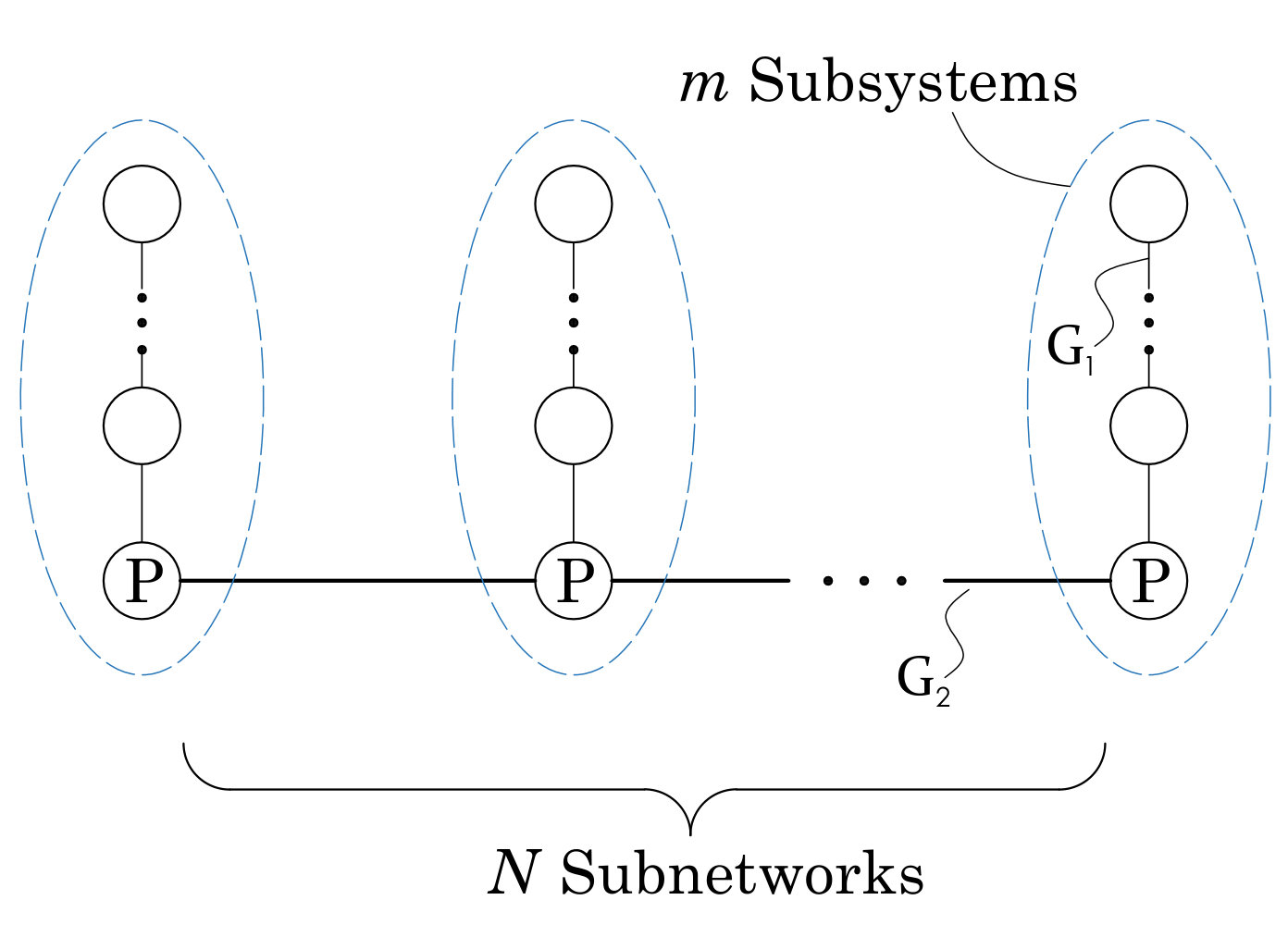 Figure 22
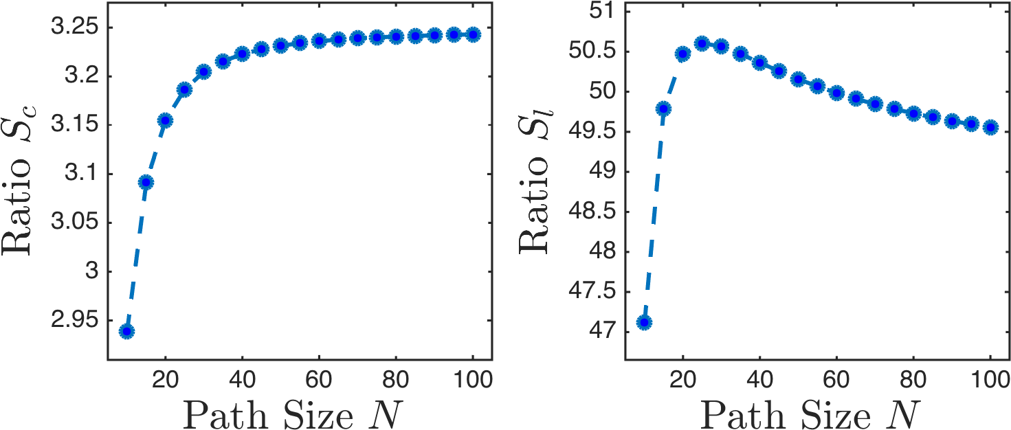 Figure 23
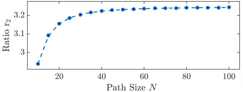 Figure 24
 Figure 25
 Figure 26
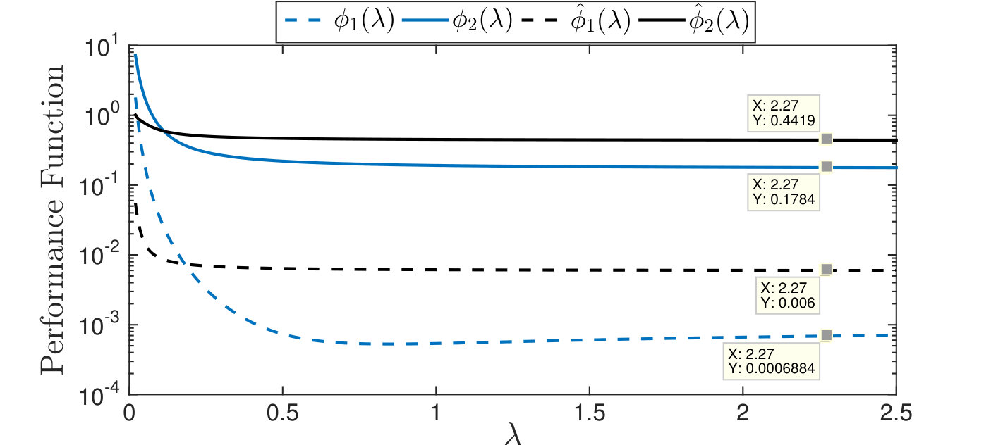 Figure 27
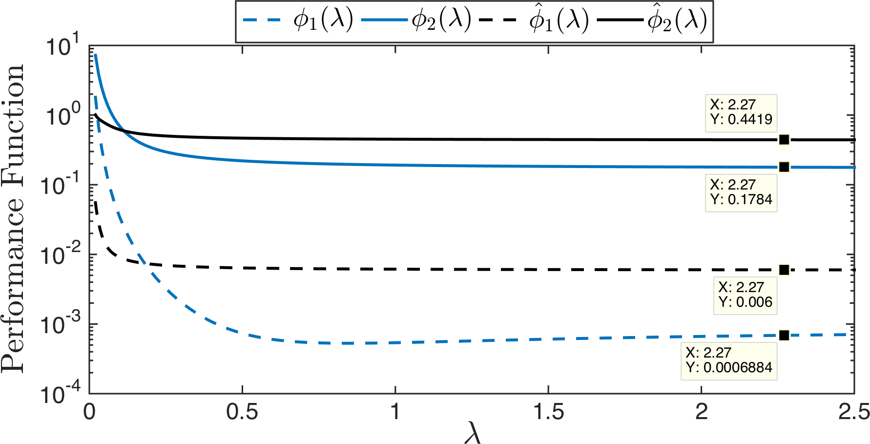 Figure 28
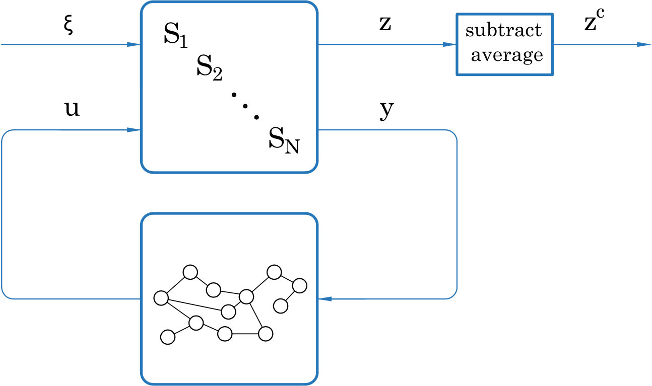 Figure 29
 Figure 30
 Figure 31
 Figure 32
 Figure 33
 Figure 34
 Figure 35
 Figure 36
 Figure 37
 Figure 38
 Figure 39
 Figure 40
| Realization | |
|---|---|
| Dynamics | Performance Function |
|---|---|
| single-integrator | |
| double-integrator |
Peer Reviews
No public reviews on file for this paper yet. If you reviewed it on a platform where reviews are public (OpenReview, ICLR, NeurIPS, ICML), you can paste yours below so the community can read it here.
Videos
No videos yet. Explain this paper in a talk, walkthrough, or lecture? Add one.
Explicit Characterization of Performance of a Class of Networked Linear Control Systems
Hossein K. Mousavi and Nader Motee1 1The Authors are with the Department of Mechanical Engineering and Mechanics, Lehigh University, Bethlehem, PA 18015, USA {mousavi, motee}@lehigh.edu
Abstract
We show that the steady-state variance as a performance measure for a class of networked linear control systems is expressible as the summation of a rational function over the Laplacian eigenvalues of the network graph. Moreover, we characterize the role of connectivity thresholds for the feedback (and observer) gain design of these networks. We use our framework to derive bounds and scaling laws for the performance of the dynamical network. Our approach generalizes and unifies the previous results on the performance measure of these networks for the case of arbitrary nodal dynamics. We bring extensions of our methodology for the case of decentralized observer-based output feedback as well as a class of composite networks. Numerous examples support our theoretical contributions.
I Introduction
Developing tools to reduce design complexity has been in the center of recent research in networked control systems [1, 2, 3, 4, 5]. In several important applications, network design problem reduces to finding an optimal communication (graph) topology among a network of identical subsystems that are coupled to each other through some common mission-related control objectives. Examples include formation control in a cooperative team of robots, the platoon of vehicles in automated highways, space-time rendezvous in a team of robots, and networks of synchronous oscillators in power networks. The design problem usually involves the optimization of a measure of performance or robustness while respecting various constraints. Due to their combinatorial nature, most network design problems become intractable as network size increases and suffer from high computational complexities. Possibility of characterizing performance and robustness measures in closed and explicit forms will significantly facilitate the design process by allowing the network designer to identify relevant functional properties of the measures and their behaviors with respect to the interconnection topology. In this paper, we present explicit expressions for the -norm, as a performance and robustness measure, of a class of interconnected network of linear control systems.
The authors of [6] consider coherency of a platoon of vehicles by evaluating the -norm of second-order consensus algorithms and propose several scaling laws for various scenarios of coordination. In [7], ill-posedness of a certain class of platoons is investigated and shown that stabilizability deteriorates as the size of the platoon increases. The string stability of a class of formation problems with limited communication range is studied in [8], where a fundamental limit on the disturbance rejection quality of the network in the frequency domain is derived. The stability and robustness of large platoon of vehicles with double-integrator dynamics are considered in [9], where it is shown that how scaling of a robustness measure (in terms of the platoon size) to external disturbances improves from geometric to polynomial growth when vehicles are allowed to communicate with their two immediate neighbors. In [10], robustness analysis and distributed controller design of platoon of vehicles with third-order models and undirected communication topologies are considered. In [11], several graph theoretic bounds on the -based performance of linear consensus networks with first- and second-order dynamics are characterized and it is shown how the performance measure scales with the network size and depends on structural properties of the communication topology. In [12], the authors consider distributed and controller design for a multi-agent system whose subsystems have general linear time-invariant dynamics. Using a consensus-like algorithm and notion of the grounded graph (e.g., see [13]) to model coupling of agents to leaders, it is shown under what conditions such controllers exist and how they can be suboptimally designed.
In this paper, we consider a network of identical subsystems that are connected over an undirected graph and subject to external disturbance and measurement noise. We propose a methodology to express the steady-state variance of the output of a class of interconnected linear time-invariant networks as a rational function of their Laplacian eigenvalues. Our method extends the existing results in the literature for first- and second-order linear consensus network models (cf. [2] and reference in there). We illustrate that the notion of minimum connectivity threshold is useful for the design of the feedback gains for these networks. It turns out that stabilizability of the nodal dynamics (and detectability in case of observer-based output-feedback) guarantee the existence of such designs. Using these developments, it is shown that fundamental limits may emerge for networks whose subsystems are non-minimum phase. We find graph-theoretic bounds for the performance of the network, which paves the way to find scaling laws for the performance measure. Moreover, a tradeoff between the graph sparsity and performance measure is revealed. Additionally, for networks over path or cycle graphs, we find the asymptotic trend of the performance measure. We bring two extensions of the analyses for the cases of observer-based output feedback as well as a class of composite networks. We have included several parametric and numerical examples to support our theoretical contributions111The proofs are included in the appendices A to P of the paper.. Our approach is advantageous for the design of these dynamical networks. Our spectral expressions can facilitate solving of underlying optimal control problems: instead of dealing directly with optimization problems with high-dimensional matrices, our method leverages the structure of the control system and decouples the roles of typically low-dimensional feedback gains and the eigenspectrum of the communication graph. This is the outgrowth of the preliminary results that were presented in the conference version [14].
II Notations and Preliminaries
The subscripts + and ++ subscripts denote the nonnegative and positive subsets of a set, respectively (e.g. ). The operator represents matrix trace. The partial ordering on the cone of positive-semidefinite matrices is denoted via and similar operators. The standard basis for is denoted by the set of vectors . The vector and matrix of ones are denoted by and , respectively. Also, and are identity and centering matrices, respectively. The vectorization is denoted by . The Kronecker product is denoted by . The matrix transpose and conjugate transpose are denoted by and superscripts, respectively. A weighted undirected graph over nodes is a collection with the following components: the set of nodes , the set of edges \mathcal{E}\subset\big{\{}\{i,j\}\;|\;i,j\in\mathcal{V}\}, and the weight function . We define and form the (symmetric) graph Laplacian with entries
[TABLE]
The set of neighbors of a node is \mathcal{N}_{i}:=\left\{j\in\mathcal{V}\leavevmode\nobreak\ \big{|}\leavevmode\nobreak\ \{i,j\}\in\mathcal{E}\right\} for . The eigenvalues of are denoted by , which are real and nonnegative for a weighted undirected graph. For a connected graph, with eigenvector , and . The Laplacian eigendecomposition is where is its orthonormal matrix of eigenvectors and For positive sequences and , we adapt if . Moreover, . Additionally, . Finally, we consider
III Problem Statement
We consider an interconnected network of subsystems where the dynamics of the ’th subsystem is governed by
[TABLE]
for , in which is the state vector of the subsystem, is the control input, is the exogenous disturbance input, is the measurement noise, is the measurable output, and is the performance output. Parameter dictates the magnitude of the measurement noise. The state of the entire network is
[TABLE]
The vectors representing the network input, disturbance, feedback noise, feedback output, and controlled output are similarly defined and denoted by , , , , and , respectively.
The control objective for the network is to achieve synchronization (or consensus), i.e., as for all . To realize this goal, we employ the following feedback control law
[TABLE]
for each subsystem . The subsystems are allowed to exchange their relative output measurements information over an undirected communication graph . It is assumed that the structure of the feedback gain matrices are restricted to where ’s are nonnegative scalars (i.e., the weights of graph ) and is the common factor among all feedback gain matrices.
When stabilizing feedback control law (8) exists and there is no disturbance and noise, one can show that as holds for the closed-loop network. However, in the presence of disturbance or noise, the state variables will fluctuate around the consensus state. To quantify these fluctuations, we look at the deviations from the average of the output states subsystems, which are given by
[TABLE]
for every . We can represent (9) in vector form as
[TABLE]
where is the centering matrix of size . The network (7) and (8) asymptotically reaches consensus if and only if asymptotically goes to zero. Since (8) can be rewritten as
[TABLE]
the controller synthesis breaks into two components: designing a feedback gain and designing a weighted undirected graph with Laplacian . It is assumed that measurement noise and noise input are both Gaussian, uncorrelated, and with independent components with unit variance. In order to measure the aggregate fluctuations in the network, we adopt the steady-state variance of the deviation from the average as a measure of performance for the design, which is defined by
[TABLE]
The research problems are to characterize performance measure (12) in terms of Laplacian eigenvalues of the underlying communication graph of the network, illustrate role of feedback (and observer) gains in stability and emergence of fundamental limits on performance and design tradeoffs, and derive scaling laws for the performance as the network grows.
IV Stability and Performance Measure Characterization
We look at the stability criteria for these dynamical networks. Moreover, we derive and characterize spectral expressions for the performance measure. For brevity, we remove the time argument from the variables.
Once we apply feedback control protocol (8), the closed-loop dynamics of the network are given by
[TABLE]
We define the auxiliary variables , , and to be
[TABLE]
Then, the following dynamical decoupling is realized (see [12] for the case of state-feedback without the measurement noise).
Proposition 1**.**
By the change of variables (14), the resulting closed-loop network dynamics given by (13) are decoupled into systems
[TABLE]
for each . In the absence of disturbance and noise, the network reaches consensus if and only if systems are asymptotically stable.
We leverage this decoupling to arrive at spectral expressions for the performance measure of the network.
Theorem 1**.**
Suppose that in (16) systems are asymptotically stable. Then, the performance measure can be expressed as
[TABLE]
with the performance function given by
[TABLE]
which is a rational function of and entries of . The map is the unique positive-definite solution to an algebraic Lyapunov equation given by
[TABLE]
for all values of that make a Hurwitz matrix.
The dimension of the dynamics of each subsystem is often small and has nothing to do with the number of subsystems. Therefore, evaluation of performance function can be done via symbolically solving Lyapunov equation (19) after converting it to a linear system by vectorization (see the proof of Theorem 1).
Due to linearity of the Lyapunov equation, one inspects that the performance function can be decomposed into two components according to
[TABLE]
in which spectral functions and only reflect the effect of disturbance and measurement noise, respectively.
Remark 1*.*
In this paper, we occasionally skip argument in and denote it as . In those cases, we solely consider the dependence of the functions on the eigenvalues of the graph Laplacian (i.e., for a fixed feedback gain ).
Remark 2*.*
A part of the result of Theorem 1 is hidden in the analysis provided in [12], in the case of state-feedback. However, the authors did not explicitly derive the spectral expressions for the performance.
We extend the previous analysis to the output-feedback and synthesize a decentralized observer. We show that the separation principal in the linear filtering using Luenberger observers is naturally carried into this design as well. Our procedure consists of four steps:
(i) We augment the dynamics of subsystem by an observer variable , whose dynamics are governed by
[TABLE]
where is an auxiliary control input for the observer. We will set the value of this input in a decentralized manner in the last step.
(ii) As it is usual in the observer design, we use to compute
[TABLE]
(iii) In addition to the relative output feedback on , the subsystems should share the value of with their neighbors. Once we consider these three steps, the augmented dynamics of subsystem are
[TABLE]
Variable has the same role as in (7); i.e., the augmented subsystems will use the relative-feedback on this variable.
(iv) We use the following theorem and design the gain of control law (8) when applied on subsystems in (25), which in this case will be an observer gain.
Theorem 2**.**
Suppose that we apply control law (8) on augmented subsystems in (25) by setting
[TABLE]
where the observer gain is set to be
[TABLE]
Moreover, assume that is chosen such that is Hurwitz for . Then, the estimation and regulation are separated: if we apply control input given in (21) for any that makes a Hurwitz matrix, then the network with this observer-based relative output-feedback reaches the consensus in the absence of disturbance and noise.
For this design, we denote the performance function by . This function can be found similar to the case of simple state-feedback, except that we need the augmented matrices of given in (25) for solving (19) and evaluation of this function.
The separation principal together with the duality between the estimation and regulation let us prove similar results for the quality of estimation using this decentralized observer. First, we define the error of estimation as
[TABLE]
Because we are only employing the relative feedback, we may only control the deviations of the error components from their average. These deviations are reflected by the variable
[TABLE]
Next, we define the estimation measure for network as
[TABLE]
The dual of system in (16) is
[TABLE]
which lets us deduce the next result (compare to Theorem 1).
Theorem 3**.**
Suppose that in (32) systems are asymptotically stable. Then, we can express the estimation measure as
[TABLE]
with the estimation function given by
[TABLE]
which is a rational function of and entries of . The map is the unique positive-definite solution to an algebraic Lyapunov equation given by
[TABLE]
for all values of that make a Hurwitz matrix.
Remark 3*.*
In [15], the authors propose the following observer-based approach. They define their observer variable to follow the dynamics
[TABLE]
and define their control law as
[TABLE]
where matrix has no eigenvalue in common with , the pair is stabilizable, and is the unique solution to Sylvester equation . Then, they design and such that a design with minimum connectivity threshold is achieved. One can see that our design is different and simpler as we only need a feedback gain and an observer gain . Moreover, our approach is built upon the separation principle between the regulation and estimation, which is also the case in the classical Luenberger (or LQG) observer design.
V Design of Control Law Gains
We investigate the problem of finding feedback gains and focus on gains inducing a minimum connectivity threshold. This property makes the design process with respect to the graph more tractable. After that, we discuss related performance limitations.
V-A * Minimum Connectivity Threshold*
We define the minimum connectivity threshold for a feedback gain to be
[TABLE]
Similar notions have been reported (e.g. [12]), while our goal is characterization of conditions for finding gains with 222 corresponds to finding the infimum of the empty set in (38).. The following definition is for this purpose.
Definition 1**.**
The feedback gain is said to have an unbounded stability region if .
If has an unbounded stability region, then the network is robust to all increases in the connectivity: if the network is output-stable for a given graph with Laplacian , then for every graph with Laplacian and , the network is still output-stable. The reason is that for (this has been emphasized in [12] as well). Moreover, this makes the stability analysis with respect to the graph more tractable, since ensuring guarantees the output-stability of network. Before bringing methods to find such feedback gains, let us look at a consequence of choosing them.
Theorem 4**.**
For a network designed with a feedback gain that in endowed by a connectivity threshold , the performance function is analytic on interval .
The openness of the interval of interest in Theorem 4 suggests that if , we need to maintain a minimum distance from this value. This will make sure that the stability margin is large enough.
V-B *State-Feedback Minimum Connectivity Design *
Let us consider the state-feedback (i.e., in (7)). It turns out that the stabilizability is the necessary and sufficient condition for existence a gain that induces a bounded threshold .
Theorem 5**.**
If is stabilizable, then for every value of , the choice of feedback gain given by
[TABLE]
satisfies , where is a solution to the following feasible linear matrix inequality.
[TABLE]
Conversely, if there exists a gain with , then is stabilizable.
The linear matrix inequality (LMI) (40) is a computational tool to find a gain for a given network and graph with a minimum connectivity threshold at most equal to (see Example 11). The solvability of LMI (40) is called the quadratic stabilizability of by means of a linear state-feedback (see Section 7.2 of [16]).
Remark 4*.*
This result is inspired by Theorem 11 in [12], while our main contribution is in pointing out the role of stabilizability in existence of feedback gains with minimum connectivity thresholds.
Remark 5*.*
The optimal choice of is not the concern in Theorem 5. Instead, we focus on the existence of designs for with a minimum connectivity design. In fact, various performance criteria could potentially get addressed. For instance, suppose that for some , we replace LMI (40) with
[TABLE]
Then, for computed from (39) using any solution to this inequality , not only , but also for each eigenvalue , the poles of have real parts less than (see [17]). As another example, authors of [12] brought a version of the matrix inequality which ensures that each decoupled subsystem has -norm less than a desired value, which they state that could be conservative in practice. Criteria such as robustness or non-fragility could be potentially added by building on top of (40) as well (e.g. see [18]).
V-C Observer-Based Minimum Connectivity Design for Output-Feedback
The duality between the derived conditions on in Theorem 2 and on in Theorem 5 lets us conclude the following result that resembles the result of Theorem 5.
Theorem 6**.**
Suppose that is detectable. Then, for every , the following observer gain for the settings of Theorem 2, has an unbounded stability region with .
[TABLE]
where is a solution to the following feasible LMI.
[TABLE]
Conversely, if under the settings of Theorem 4 an observer gain has a bounded , then is detectable.
The LMI (43) is the quadratic stabilizability condition for the dual pair 333It is stabilizable since pair is detectable.
V-D *Asymptotic Performance and Estimation Bounds *
An important design question is if the performance function can be made arbitrarily small, which is related to the notion of almost disturbance decoupling [19]: attenuating the effect of the disturbance in a performance metric as much as desired. We study the case of relative state-feedback below.
Theorem 7**.**
Suppose that is stabilizable and is detectable and that . For all pairs of and for which is Hurwitz, the performance function resulting from the relative state-feedback is bounded from below according to
[TABLE]
for a positive semi-definite matrix given by
[TABLE]
where is the unique positive semi-definite solution to the parametric algebraic Riccati equation
[TABLE]
Matrix is zero if and only if transfer matrix is right-invertible and minimum-phase.
For instance, if the transfer matrix is non minimum-phase and the columns of are not in the null space of , then the bound in (44) is strictly positive. The dual of this result for estimation quality is given below, whose proof is identical to Theorem 7.
Theorem 8**.**
Suppose that is stabilizable and is detectable. If for some gain , are Hurwitz for , then
[TABLE]
for a positive semi-definite matrix given by
[TABLE]
where is the unique positive semi-definite solution to the parametric algebraic Riccati equation
[TABLE]
Matrix is zero if and only if transfer matrix is right-invertible and minimum-phase.
V-E * Parametric Evaluation of *
In both relative state or output feedback designs, if is not large (e.g. 1 to 4), we may design with an unbounded stability region using Routh-Hurwitz criteria and explicitly evaluate . In fact, the characteristic equation of the matrix for the decoupled systems for eigenvalue is
[TABLE]
They must be Hurwitz polynomials for . As we enforce the Routh-Hurwitz criteria, we find a set of essentially nonlinear inequalities involving and elements of , such that the minimum connectivity threshold is realizable and evaluable based on values of (see the next section for examples).
VI Examples of Performance Analysis
In this section, we bring different classes of subsystems and characterize their performance within this framework. We bring additional details of the examples in Appendix Q.
First, we consider two single-input single-output controllable subsystems under the relative state-feedback, where the disturbance and control input drive the dynamics from the same channel (without the measurement noise).
Example 1*.*
Consider the subsystems given in Table I, where we have also reported the corresponding performance functions. For the nodal dynamics and , supposing that and , respectively, in both cases . Moreover, for , performance function is strictly convex and strictly decreasing. If all ’s are zero and , these subsystems are called single and double-integrators, respectively. As a numerical example, let us consider double-integrators with . Then, using the second row of Table I we get
[TABLE]
This is a well-known result (e.g. see [20]).
Example 2*.*
Consider double-integrators with relative feedback only on positions () using the decentralized observer of Theorem 6. We let and set the observer gain to be . Theorem 2 requires the stability analysis for matrix , which is Hurwitz if and only if . Then, we get . We can show that
[TABLE]
where to are polynomials of and . Using the observer with , (51) becomes
[TABLE]
One observes that for weak connectivity regimes (i.e., near zero), in (52) is close to the function in (50), while as increases, the performance function corresponding to relative state-feedback vanishes, while the function from observer design does not.
Example 3*.*
We consider a triple-integrator with dynamics
[TABLE]
Let us choose the state to be with element-wise positive gain . We can show that
[TABLE]
The next two examples also have performance functions that under conditions become strictly decreasing and convex.
Example 4*.*
The dynamics of a harmonic oscillator of mass are governed by
[TABLE]
where is the damping ratio and is the undamped angular frequency (see [21]). We consider and compute with the relative state-feedback on with . Using arguments similar to Example 1, if we define and we get
[TABLE]
Again, for element-wise positive feedback gains, is strictly convex and strictly decreasing for .
Example 5* (Platoon of Vehicles).*
We consider a network of vehicles, in which the position of ’th vehicle is denoted by . It has the third-order dynamics
[TABLE]
where the input is the desired acceleration and is the disturbance. The time-constant characterizes how fast the vehicles responds to the acceleration command. The state vector is chosen as , where they denote the (errors in) the position, velocity, and acceleration of the vehicles in the platoon, respectively (see [10] for more details). The state-space matrices are given in the appendix. Using relative state-feedback, by application of the Routh-Hurwitz criteria we find that if satisfies we get
[TABLE]
We can show that if , we get
[TABLE]
If , the design corresponds to a relative output-feedback on only positions and velocities, with a performance function
[TABLE]
which is strictly convex and strictly decreasing for . If , we have the relative state-feedback and for the same argument holds (see the appendix).
Example 6*.*
Consider a network with nodal matrices
[TABLE]
for and . We observer that the subsystems have a non minimum-phase input-output transfer function
[TABLE]
where is the location of the right-hand plane zero. Let us consider the relative state-feedback. We can show that in this case, we have . For a disturbance matrix , Theorem 7 gives us the bound
[TABLE]
Alternatively, if we use the relative state-feedback, we can show that the corresponding performance function is
[TABLE]
which is strictly convex and decreasing for . Now, for any gain with an unbounded stability region
[TABLE]
where . By differentiation with respect to , we find that the right side attains its minimum at . Thus
[TABLE]
which is the same bound as (62). The bound on the performance function scales with the magnitude of the right-hand plane zero at . One inspects that if the disturbance enters the subsystem from the same channel as the control input, we do not face a fundamental limitation on the performance, because in this case it does not touch the zero dynamics of the subsystems (see [22] for a similar observation in the case of -norm).
Example 7*.*
In this example, first, we consider two different designs for a network of double-integrator agents with measurement noise. Recall that the magnitude of feedback noises is controlled by parameter .
(i) the relative state-feedback without the filtering (i.e., without the decentralized observer): in this case, using , we can show that
[TABLE]
in which the first term can be recovered from Table I and the second term appears due to the measurement noises.
(ii) the relative output-feedback on positions with the decentralized observer: in this case
[TABLE]
in which is the performance function read from (51) and to are polynomials of ’s and ’s. For instance, in the case of , this function becomes
[TABLE]
Next, we find estimation function . We can show that
[TABLE]
The first term is due to the disturbances, while the second term originates from the feedback noises. The transfer matrix is right-invertible and minimum-phase. Hence, as Theorem 8 suggests, as becomes smaller, we can make the estimation arbitrarily precise by increasing the magnitude of observer gains and .
VII Analysis of Network of Networks
We introduce and analyze a class of networks of networks that are built by a repeated application of control law (8). For simplicity of the developments, we neglect the feedback noises (i.e., set ). One can show that the same approach works in the presence of those noises as well.
VII-A Construction Procedure for Composite Networks
First, we build identical networks using control law (8) over graph . We denote the number of nodes of by and the order of the state-space realization for each subsystem by . Moreover, we denote the feedback gain used to build each network by . Let us denote the state of subsystem in module or subnetwork by . Similarly, we denote the rest of corresponding variables. The Laplacian matrix corresponding to is also denoted by . For the subsequent analysis, let us define
[TABLE]
According to (13), the dynamics of the subnetwork are
[TABLE]
where is the state vector of module and disturbance vector is defined similarly. Without loss of generality, we designate the last node in graph as the port of the module444 If we wish to choose another node, we can simply relabel the nodes., which corresponds to a subsystem that we can add a term to its control input. This converts (70) to new open-loop dynamics
[TABLE]
wherein is the tunable control input to the module. Moreover, we assume that two modules can become interconnected only through their port nodes. Then, the only variable that module can use for relative feedback is the output variable for the port node, which is denoted by
[TABLE]
We collect instances of these networks with dynamics (71) and feedback variables (72) to construct a composite network. Therefore, the subsystems equivalent to in (7) for this network design are
[TABLE]
with the structured matrices defined by (69). Now, we build a modular network by application of control law (8) with modules (or subnetworks) connected over a higher level graph with feedback . 555 Feedback gains and are matrices of the same dimension because we have chosen one node as the port of a subnetwork. If has a weight denoted by , then the application of control law (8) will be
[TABLE]
We have modules and each one consists of subsystems. Therefore, the consensus output of the network should be
[TABLE]
Then, we set its steady-state variance as the performance measure
[TABLE]
where is the graph Laplacian of . In Fig. 1, we illustrate this composite structure using an example: we have four modules and inside each of them, three subsystems are interconnected over graph , in this case a complete graph. These subnetworks are then connected via their ports over graph , which in this case is a path.
*Interpretation of Construction: * Let say modules and are connected, thus . Then, the ports of these two modules will have access to the relative difference of their feedback output and will reflect this feedback term in their control input. Mathematically speaking, the input to the port node666 Recall that the port node is arbitrary chosen or labeled to be number . in module is
[TABLE]
The first term is due to initial application of control law (8) over with an edge set , while the second term is from (77) based on the composite network design over .
VII-B Stability and Performance of Composite Networks
Theorem 9**.**
Consider a dynamical network over graph with a bounded performance measure . Suppose that in Proposition 1 and Theorem 1 we apply control law (8) on systems defined in (76) over with feedback gain . The resulting composite network reaches consensus if and only if is Hurwitz for nonzero eigenvalues of . Moreover, if is the performance function derived from Theorem 1 for subsystems defined in (76), then
[TABLE]
The significance of this result is that for a fixed module graph with Laplacian and , the value of and the form of composite performance function are fixed. Thus, we can quantify the role of higher level graph and feedback gain in the performance of the composite network by looking at the second term. The extra term compared to Theorem 1 appears because
[TABLE]
where the right-hand side is the output that would have resulted in an expression of form (17).
Remark 6*.*
If a subnetwork is one subsystem, then (81) reduces to (17), since each subsystem as a network satisfies .
VII-C * Minimum Connectivity Design For Composite Networks*
We show that if , then there exists a simple choice for such that it has also an unbounded stability region in terms of the eigenvalues of higher level Laplacian ; i.e., exists and if then is Hurwitz. This would remedy the concerns about possible complexities in the design of over graph .
Theorem 10**.**
Suppose that the subnetworks are built over any graph and feedback gain , which has an unbounded stability region. For any , let us choose the feedback gain of the composite network to be . Then, has an unbounded stability region with respect to the eigenvalues of higher level Laplacian .
This result is simplified if .
Corollary 1**.**
Suppose that the subnetworks of the network of networks are built with , which induces . Let us choose for some in the design of the described composite networks. Then, higher level feedback gain satisfies with respect to the eigenvalues of higher level Laplacian .
VII-D * Examples of Networks of Networks*
Example 8*.*
Consider a modular network with subnetworks of single-integrators over an unweighted path graph of nodes, where the last node of the module is its port. We choose so the open-loop dynamics of the modules before design of the composite network based on (71) are
[TABLE]
where , , and is Laplacian of the unweighted path graph over nodes. Then, choosing , the performance function of the composite network is
[TABLE]
Based on Corollary 1 in the higher level . Moreover, we inspect that the resulting family of functions is strictly convex and decreasing for (see the appendix for the details).
Example 9*.*
Consider a modular network, where each subnetwork consists of subsystems with the single or double-integrator dynamics. In this case, we set to be the unweighted complete graph over nodes (similar to the example illustrated in Fig. 1 for the subnetworks with ). Therefore, unlike Example 8, no matter which node is chosen as the port, the subnetwork will be the identical. For element-wise positive feedback gains and , Corollary 1 again implies that the minimum connectivity threshold in terms of the eigenvalues of for both nodal dynamics is zero. Moreover, let for the single-integrators and for the double-integrators (for simplicity). Using the solution to the Lyapunov equation, we find performance function for these subnetworks, which are e given in Table II. These functions are strictly convex and decreasing for . As a sanity check, for the unweighted path and complete graphs coincide and the first formula in Table II and (84) produce identical functions for (see appendix Q for details).
VIII Performance Bounds and Scaling
We look at the cases where combining the information on graph parameters and derived performance functions can give us macroscopic information on the performance measure.
VIII-A * Performance Bounds and Scaling *
In Sections VI and VII, a majority of the derived performance functions are convex. In what follows, we show that this property is useful in derivation of performance bounds.
Theorem 11**.**
Consider a network of subsystems with a performance functions that is convex. The performance measure over an unweighted graph with edges and maximum nodal degree of is lower-bounded according to
[TABLE]
where the equality holds if and only if graph is either complete graph or star graph.
Example 10*.*
Consider a network with nodal dynamics , and . For all connected unweighted graphs with to nodes, we do a survey for the ratio of the sides of inequality (85), that is
[TABLE]
The distribution of versus is illustrated in Fig. 2. As increases, it tends to an almost fixed curve (with a growing tail), where of the graphs induce a ratio .
Theorem 12**.**
Consider a network of subsystems with a performance functions that is convex. The performance measure over any weighted graph with a total weight of is lower-bounded according to
[TABLE]
*where the equality holds if and only if the graph is complete and with identical weights. *
Theorems 11 and 12 give rules of thumb about the best achievable performance. To do so, we combine information on the nodal dynamics (through the form of the performance function) and macroscopic graph information.
Corollary 2**.**
Under the settings of Theorem 12, it holds that
[TABLE]
Performance-Sparsity Tradeoff: Suppose that is also decreasing. For an unweighted graph, . Therefore, we can reorganize the result of Theorem 12 and write
[TABLE]
This result is useful in quantification of the following tradeoff: as the graph of the network becomes sparser, the best attainable value of the performance measure will increase. The following example highlights two specific cases.
Example 1 (Continued)**.
For networks with subsystems that have dynamics, Corollary 2 implies that over any unweighted graph
[TABLE]
For networks with subsystems of dynamics we deduce
[TABLE]
For instance, in the special case of for we get
[TABLE]
that clearly reflects the sparsity-performance tradeoff for a consensus network of double-integrators (see [11] for a similar result for single-integrator agents).
VIII-B * Performance Asymptotic over Path and Cycles*
Theorem 13**.**
For a network of subsystems over an unweighted path or cycle graph with , it holds that
[TABLE]
where can be computed using a parametric integral
[TABLE]
Moreover, if is bounded at , then it holds that
[TABLE]
Corollary 3**.**
The performance measure scales similarly with respect to over unweighted path and cycle graphs. Moreover, if is bounded at [math], the performance measure over the paths and cycles converge to the same value as .
We should emphasize on few points: (i) Theorem 13 does not depend on neither convexity nor monotonicity of ; (ii) the requirement is natural, since as increases ; i.e., it becomes arbitrary small. Otherwise, there exist such that for , . (iii) This approximation idea has been previously reported, e.g. in [23] it is used for estimation of Estrada index. However, we find the reason for which the approximations find the scaling of the sums, even if is singular at .
Example 1 (Continued)**.
We apply Theorem 13 on a network of subsystems with (i.e., single-integrators) over an unweighted path and arrive at the asymptotic expression
[TABLE]
while if , for , we have the approximation
[TABLE]
For agents with , the performance measure satisfies
[TABLE]
Next, for these agents with over an unweighted path graph of nodes, we investigate the claim of Theorem 13 by looking at the ratio
[TABLE]
with given in (99). The result is shown in Fig. 3, where according to Theorem 13, indeed goes to a constant.
Example 4 (Continued)**.
For a network of harmonic oscillators with over a path graph, Theorem 13 implies that
[TABLE]
We call the right hand side . To empirically examine the gap, we consider
[TABLE]
We set , for , and vary between and . Because is bounded, as increases the approximation becomes tighter as shown in Fig. 4.
Example 5 (Continued)* (Platoon over a Path).*
For a platoon of vehicles over a path graph, Theorem 13 suggests that scales with . Thus, the -norm scales with . As reported by the authors in [10], a similar scaling law in the case of norm of the network over this topology holds (with an additional leader).
Example 7 (Continued)**.
We can apply Theorem 13 to find the scaling for the estimation measure as well. Similar to (99), we can show that the estimation measure in a network of double-integrators over a path graph satisfies
[TABLE]
Example 8 (Continued)**.
We consider a network of subnetworks over a path graph, where the subsystems are a network of single integrators, also over a path graph with subsystems as analyzed in Example 8. This network is illustrated in Fig. 5. From (97), we already know that the performance of isolated subnetworks satisfies
[TABLE]
Combining (103) and Theorem 7, we can show that
[TABLE]
IX Application to Formation of Aircraft
Example 11* (Formation of Aircraft).*
We consider a linearized model for the dynamics of an aircraft [24] expressed as
[TABLE]
where (see Appendix Q for the numerics). The variable is the horizontal velocity component from its set point and is the component normal to that. The pitch angle is denoted by . The control inputs and are the elevator angle and thrust force, respectively. The scalars and denote the wind velocity in the longitudinal and lateral directions, respectively. We consider the formation shown in Fig. 6. Once each vehicle takes into account the relative distances from their neighbors (in computation of the position feedbacks), we can use these dynamics to analyze the performance of this network with the performance output
*Relative State-Feedback: * We use the convex optimization toolbox CVX [25] to find for using Theorem 5. If and have intensity of unity, we get
[TABLE]
where and describe the magnitude of the fluctuations in the formation in and directions, respectively. The performance functions are rational functions with the numerator and denominator of order 9. While it is guaranteed to get , we have . In Fig. 7, we plot and , where for larger values of , they are different by more than an order of magnitude. The function is convex and decreasing, while is neither strictly convex nor monotone for . This suggests that properties of these functions in general could be beyond a simple classification.
*Observer-Based Relative Output-Feedback: * next, we consider the observer-based output-feedback on the last two states of each subsystem (i.e., horizontal and vertical relative positions). For the value of we reuse its value from the previous design. We choose observer gain for using Theorem 6 and find that
[TABLE]
where these two functions are also depicted in Fig. 7. In this case, as well. In Fig. 8, we demonstrate two sample longitudinal output plots based on these two designs, where we have planes that are supposed to travel with . The graph is a path with weights of and identical disturbance samples are fed into the subsystems in two cases. The different level of fluctuations is justifiable upon comparison of the values of and in Fig. 7.
X Conclusion and Discussion
We brought a unifying framework for performance analysis of a class of networked control systems. The resulting spectral expressions let us derive bounds and scaling laws for the performance of the system. We would like to include a a number final remarks:
(i) The spectral expressions for the performance measure can be used to find the optimal values of feedback gain . In fact, for large networks, solving the Lyapunov equation for the performance measure once the value of feedback gain is updated could be computationally expensive. Instead, suppose that we find the spectral expressions for the performance measure for a fixed graph. Then, our objective function will be a scalar function of the feedback gain. The resulting problem can be effectively approached using general nonlinear problem methods. This approach is also useful when solving for optimal observer gains or feedback gains for composite networks and when the graph is fixed. The gains derived from the linear matrix inequalities given in Section V can be used as a starting point of the optimization procedure.
(ii) We can derive similar spectral expressions for the variance of the control input that is consumed throughout the network in the steady-state, which is given by
[TABLE]
Then, we can show that
[TABLE]
for rational input function given by
[TABLE]
The map is the solution to (19). For instance, we can show the input functions for networks of single-integrators and double-integrators are given by
[TABLE]
respectively. The developments in this paper which has to do with the performance functions can be applied to the input functions as well (e.g. asymptotic control input over a path).
(iii) In cases that symbolic evaluation of the performance functions is computationally prohibitive, an alternative option is to conduct regression to estimate the coefficients of these rational performance functions numerically.
Appendix A
Proof of Theorem 1: Let us define The transfer matrix from disturbance and noise to consensus output can be expressed as
[TABLE]
where is the transfer matrix from to . This lets us compute the following quantity
[TABLE]
The matrix is simply given by
[TABLE]
Taking from the both sides results in
[TABLE]
Due to cyclic property of the trace, the first and last matrix in the trace argument cancel out and we get
[TABLE]
The last norm term can be computed using the state-space formulation of systems . This will be the Lyapunov equation (19) [26]. Therefore, we have managed to prove
[TABLE]
Next, we prove that is a rational function. The Lyapunov equation (19) upon vectorization becomes
[TABLE]
Using the Cramer’s rule, for , we may compute the ’th element of as
[TABLE]
where is the matrix derived by replacing column of with . Both numerator and denominator are polynomials of with coefficients that are polynomials of the elements of . Therefore, the same conclusions holds about .
Appendix B
Proof of Theorem 2: If we apply control law (8) for the new subsystem with observer gain (partitioned based on ), we have the following formula
[TABLE]
This means that corresponding to the dynamics are
[TABLE]
Defining the error as , we get that
[TABLE]
The subsystems in the consensus problem have reduced to the familiar decoupled Leunberger observer/regulator form (e.g. see [27]). Therefore, we need to simultaneously have: for and to be Hurwitz. Then, the corresponding is asymptotically stable for and the network reaches the consensus.
Appendix C
Proof of Theorem 3: If we consider the dynamics of in (110), they are identical to dynamics of in (32). The rest of the proof is similar to Theorem 1 once we replace with .
Appendix D
Proof of Theorem 4: The definition of implies that for all , subsystems to are asymptotically stable. Therefore, the performance function is bounded. Because is rational, it is analytic everywhere in its domain, including this interval.
Appendix E
Proof of Theorem 5: First, for a linear time invariant control system the feasibility of the linear matrix inequality and the stabilizability are equivalent [16]. The second part of the claim is a special case of Theorem 11 in [12] with only accounting for the stabilizablity of the subsystems, so we do not repeat the proof in this manuscript. The converse argument holds because if , then for , is Hurwitz; i.e., is stabilizable.
Appendix F
Proof of Theorem 6: Due to duality of between the stabilizability and detectability, if the pair is detectable, then is stabilizable. Now, we can use the same argument as Theorem 5 to complete the proof.
Appendix G
Proof of Theorem 7: Consider the control system
[TABLE]
Saberi et. al. [28] have shown that the minimum value of the norm for this system is where can be computed as the solution to an algebraic Riccati equation
[TABLE]
Moreover, it has been shown that if is stabilizable and is detectable, then converges to zero if and only if the mentioned transfer matrix is right-invertible and minimum-phase. Now, we should note that the performance function is the norm squared of a system similar to (113), expect that we have . Under this modification, the limiting case for in Riccati equation (114) does not change.
Appendix H
Proof of Theorem 9: Let us denote orthonormal eigendecompostion of Laplacian by . The decoupled system in this case is
[TABLE]
Let us call the transfer matrix from to by . Then, the transfer matrix from disturbance to performance output in the case of network of networks can be written as
[TABLE]
This lets us compute the following quantity
[TABLE]
We take the trace and move the first two terms of the trace argument to the right to get
[TABLE]
The intermediate term can be simplified according to
[TABLE]
Hence, we can further write
[TABLE]
If we take the map from the sides
[TABLE]
For , and the system will have a transfer matrix from the disturbance to output . Moreover, in this case has the closed-loop dynamics of the subnetworks. Therefore, we inspect that
[TABLE]
Additionally, we observe that for , we have
[TABLE]
provided that is the performance function computed using matrices in (69).
Appendix I
Proof of Theorem 10: If , then we can consider the network of network to be a single network with feedback gain , over a graph . The weights of links in are preserved, while the weights of the links in are scaled by . Hence, if we increase the weights in the higher level network (equivalently, the eigenvalues of ), at some point the second smallest eigenvalue of equivalent Laplacian will pass .
Appendix J
Proof of Corollary 1: Following the same lines as in the proof of Theorem 10, if the minimum connectivity threshold is zero, for any choice of , the network with a single equivalent graph and feedback gain has zero minimum connectivity threshold, while the equivalent Laplacian would always have a nonzero . Hence, the connectivity threshold in terms of the eigenvalues of is zero as well.
Appendix K
Proof of Theorem 11: First we proof an inequality that is an extension of one in [29] in the case of for . For a continuously differentiable convex function and a Laplacian with edges and maximum degree , we show that
[TABLE]
and the equality holds if and only if is complete or star. The steps provided in the proof of this lemma are essentially the same steps reported for Theorem 3 in [29] (only for power functions). Since is convex and continuous, we use Jensen’s inequality to write
[TABLE]
where if the function is not affine, then the equality holds if and only if . This implies we can write
[TABLE]
where the auxiliary function is defined as
[TABLE]
Because is continuously differentiable, so is and
[TABLE]
The function is convex, thus is nondecreasing. Then, is strictly increasing, since for any
[TABLE]
In an unweighted graph, (see [29] and also [30]). Therefore,
[TABLE]
which proves 115. Applying this on a convex , (85) is followed. The equality holds if and only if and , which happens if and only if is either complete or star (again, see both [29] and [30]).
Appendix L
Proof of Theorem 12: Consider any convex function . We start from Jensen’s inequality in the form of
[TABLE]
Because the eigenvalues sum to , replacing with gives us the inequality (86). The equality holds if and only if that happens if and only if is complete graph with identical weights.
Appendix M
Proof of Theorem 13: For an unweighted path graph
[TABLE]
We define the equidistant partition of interval as
[TABLE]
We define the following quantities for each interval:
[TABLE]
They induce the following summations
[TABLE]
where . These sums imply the natural ordering
[TABLE]
Moreover, compared to , we observe that
[TABLE]
We bring a lemma whose proof is given in the next appendix.
Lemma 1**.**
For a rational function that is bounded for any , uniformly over and for some depending on .
We can apply Lemma 1, since . As a results, we find that
[TABLE]
This means that and are both bounded according to
[TABLE]
If we combine these two inequalities, we find that
[TABLE]
If is bounded, then one deduces that
[TABLE]
Therefore, we can write the following two inequalities
[TABLE]
[TABLE]
Thus, we can write
[TABLE]
For unweighted cycle graphs, the Laplacian eigenvalues are
[TABLE]
Without loss of generality, for deriving the scaling purposes, we may assume that is . Then, we will have distinct values for the eigenvalues of , where each value is repeated exactly twice. Moreover, we can write
[TABLE]
This time, we need to partition and proceed with identical steps to find out that does the same job in the case of cycle graphs. If we replace , the factor is canceled. This means that (94) and (96) upon replacement of with are achieved, where
[TABLE]
Since , the same conclusion apply for the networks over cycle graphs as well.
Appendix N
Proof of Lemma 1: Let us define and Denote the order of the pole of at by . This means that we can decompose according to
[TABLE]
for some strictly positive function that is bounded and rational. We can write this in terms of as follows
[TABLE]
In the interval of interest, , (a bounded and positive rational function) and are all Lipschitz continuous, so is their composition . This implies that is Lipschitz-continuous. Hence, for and , the corresponding Lipschitz continuity inequality will be
[TABLE]
for some Lipschitz constant . This is equivalent to
[TABLE]
This means that alternatively we may write
[TABLE]
Let us define
[TABLE]
Since is increasing in , for
[TABLE]
Moreover, one can find that is decreasing for any . Thus, we can write
[TABLE]
We can see note that the right hand side of (120) is
[TABLE]
Computing its formal derivative with respect to , we get
[TABLE]
Thus, its supremum should be evaluated based on the limit
[TABLE]
Let us take the maximum of the left hand side of (119) over and combine it with (121). We conclude that
[TABLE]
which completes the proof.
Appendix O
Proof of Corollary 3: Because and scale similarly with respect to , the first part of the claim follows. If the performance function is bounded, then both of them become the same quantity, because we can replace the lower bound of these two integrals with a common limit of [math].
Appendix P
Proof of Result on Input Measures.
We can see that
[TABLE]
We can further write
[TABLE]
Because , we can write
[TABLE]
If we take the expected value and tend the time to infinity, using the same lines as the proof of Theorem 1, we find that
[TABLE]
Let us take the trace from the both sides. We find that
[TABLE]
Because , we conclude that
[TABLE]
Let us move to the left hand side of the trace arguments. The claim is followed. ∎
Appendix Q:
Additional Details of Examples
Details of Example 1: For networks with nodal dynamics , the noiseless dynamics of are
[TABLE]
that are asymptotically stable if . This confirms . The solution to (19) is which result in the claimed form for . We can see that for , it is strictly convex and strictly decreasing. The dynamics of the subsystem for nodal dynamics without disturbance and noise are
[TABLE]
The corresponding characteristic polynomial is
[TABLE]
which is a stable polynomial if and only if that imply . Using (19), we get that
[TABLE]
Substitution of this matrix into (18) gives us the results of the table. Now, noting that
[TABLE]
that is sum of two strictly convex and strictly decreasing functions after their negative poles. Those poles are less than or equal to . Hence, the is strictly decreasing and strictly convex in the claimed domain.
For the double integrator with observer, note that
[TABLE]
Observe that its characteristic polynomial is which is stable if and only if .
Details of Example 3: For the network of triple-integrators, the characteristic polynomial is
[TABLE]
The stability requires and
[TABLE]
The solution to for from the Lyapunov equation is shown in Table III. The formula for the performance function then is followed by computing .The performance function in this case is strictly decreasing and convex.
Details of Example 5: The realization of the agents is
[TABLE]
The characteristic polynomial of the systems in this case becomes
[TABLE]
(see also [10]). Based on Routh-Hurwitz criteria, for an unbounded stability region, we should impose the following restrictions on . Moreover, we need the inequality
[TABLE]
from which we may infer the bicriteria definition for in (60). To find the performance functions, we find which is
[TABLE]
which lets us compute the performance function. If , the function is a positive combination of
[TABLE]
Moreover, and are products of functions that are strictly convex and decreasing for according to
[TABLE]
Thus, the performance function is this case is also strictly convex and strictly decreasing for .
Details of Example 6: The input-output transfer function is with a right-hand plane zero at . To evaluate , we use a method suggested by [31]. First, we decompose the transfer function according to where the components are
[TABLE]
The transfer function has the balanced realization 777A minimal realization of a stable transfer matrix is called balanced if its controllability and observability Gramians are diagonal and equal (such a realization exists for a stable transfer matrix).
[TABLE]
while has a stabilizable and detectable realization
[TABLE]
Suppose that the factorized realizations have the state vectors and , respectively. Then, we can show that they are related based on
[TABLE]
Then, the reference shows that
[TABLE]
Therefore, we get
Details of Example 8: We can see that and
[TABLE]
The solution to the Lyapunov equation in this case is
[TABLE]
Now, similar to the previous example, we can see that
[TABLE]
Details of Example 9: For subnetworks of single-integrators over that is complete, and
[TABLE]
We can verify that the solution to the Lyapunov equation is
[TABLE]
Then, we can write
[TABLE]
For double-integrators over complete graph modules, similar expressions for the matrices , and holds, while the solution to the Lyapunov equation in this case is shown in Table IV. Because the output of the double-integrator is on the first state, we can write
[TABLE]
This proves the claims in the example.
Details of Continuance of Example 1: First, we prove that we can replace in Theorem 13 with
[TABLE]
Considering , we get that
[TABLE]
Given , and
[TABLE]
that are integral limits of interest.
Now, if , for the single integrators
[TABLE]
we can compute for as
[TABLE]
Now, if , then we need the integral
[TABLE]
This implies that for in this case satisfies
[TABLE]
For agents with we need
[TABLE]
Now, we compute for as follows
[TABLE]
Details of Continuance of Example 4: In this case similar computations reveals that for
[TABLE]
Details of the Continuance of Example 8: In this case,
[TABLE]
Thus, based on the formula for the performance of the network of networks in (81), the claim is followed.
Details of Example 11: The state space matrices of the aircraft model are borrowed from [24] are given below.
[TABLE]
The result of feedback gain design is
[TABLE]
For the case of observer-based relative output feedback, the following value of gives us depicted performance functions.
[TABLE]
The reference list from the paper itself. Each links out to its DOI / PubMed record.
- 1[1] M. Siami and N. Motee, “Network abstraction with guaranteed performance bounds,” IEEE Transactions on Automatic Control , vol. 63, no. 10, pp. 3301–3316, 2018.
- 2[2] ——, “Growing linear dynamical networks endowed by spectral systemic performance measures,” IEEE Transactions on Automatic Control , vol. 63, no. 7, pp. 2091–2106, 2017.
- 3[3] A. Jadbabaie and A. Olshevsky, “Scaling laws for consensus protocols subject to noise,” IEEE Transactions on Automatic Control , vol. 64, no. 4, pp. 1389–1402, 2018.
- 4[4] M. Fardad, F. Lin, and M. R. Jovanović, “Design of optimal sparse interconnection graphs for synchronization of oscillator networks,” IEEE Transactions on Automatic Control , vol. 59, no. 9, pp. 2457–2462, 2014.
- 5[5] M. Andreasson, E. Tegling, H. Sandberg, and K. H. Johansson, “Performance and scalability of voltage controllers in multi-terminal hvdc networks,” in 2017 American Control Conference (ACC) . IEEE, 2017, pp. 3029–3034.
- 6[6] B. Bamieh, M. R. Jovanovic, P. Mitra, and S. Patterson, “Coherence in large-scale networks: Dimension-dependent limitations of local feedback,” IEEE Transactions on Automatic Control , vol. 57, no. 9, pp. 2235–2249, 2012.
- 7[7] M. R. Jovanovic and B. Bamieh, “On the ill-posedness of certain vehicular platoon control problems,” IEEE Transactions on Automatic Control , vol. 50, no. 9, pp. 1307–1321, 2005.
- 8[8] R. H. Middleton and J. H. Braslavsky, “String instability in classes of linear time invariant formation control with limited communication range,” IEEE Transactions on Automatic Control , vol. 55, no. 7, pp. 1519–1530, 2010.