Creation of knowledge through exchanges of knowledge: Evidence from Japanese patent data
Tomoya Mori, Shosei Sakaguchi

TL;DR
This paper provides empirical evidence that direct exchanges of differentiated knowledge among Japanese researchers enhance collaborative patent output, increasing both quantity and novelty, with different mechanisms for each.
Contribution
It demonstrates how knowledge exchanges specifically boost collaborative productivity in patent creation, measured by quality and novelty, using Japanese patent data.
Findings
Knowledge exchange increases the number of patents (extensive margin)
Knowledge exchange enhances patent novelty (intensive margin)
Different mechanisms drive quality and novelty improvements
Abstract
This study shows evidence for collaborative knowledge creation among individual researchers through direct exchanges of their mutual differentiated knowledge. Using patent application data from Japan, the collaborative output is evaluated according to the quality and novelty of the developed patents, which are measured in terms of forward citations and the order of application within their primary technological category, respectively. Knowledge exchange is shown to raise collaborative productivity more through the extensive margin (i.e., the number of patents developed) in the quality dimension, whereas it does so more through the intensive margin in the novelty dimension (i.e., novelty of each patent).
Click any figure to enlarge with its caption.
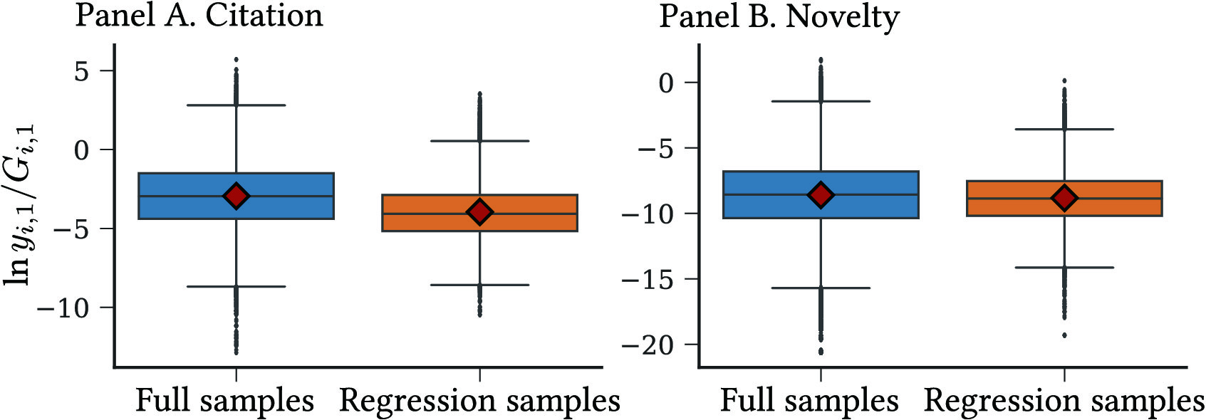 Figure 1
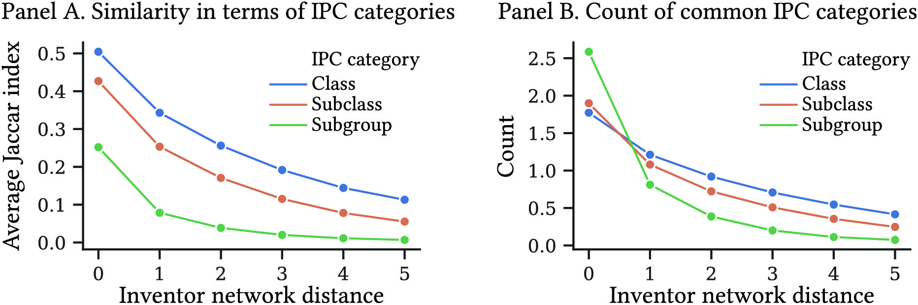 Figure 2
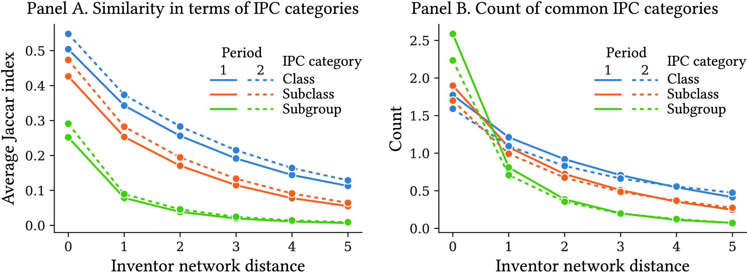 Figure 3
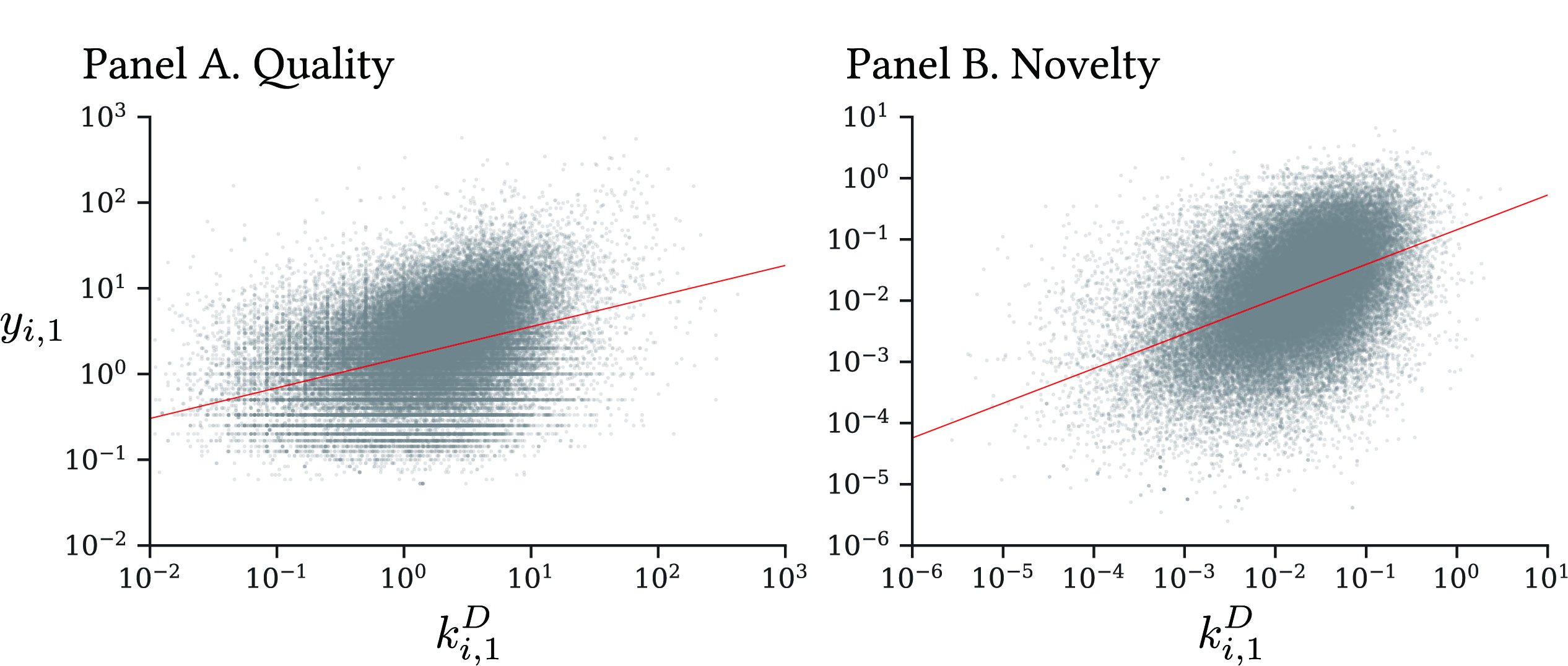 Figure 4
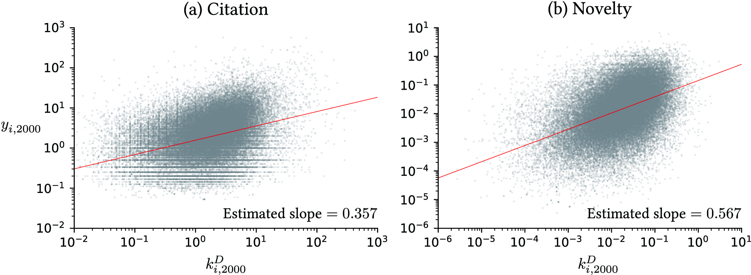 Figure 5
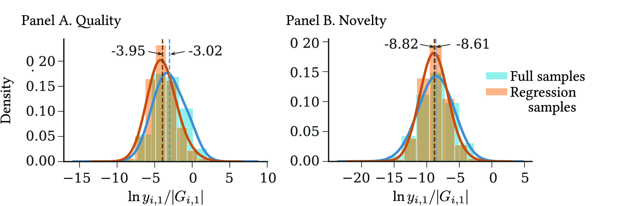 Figure 6
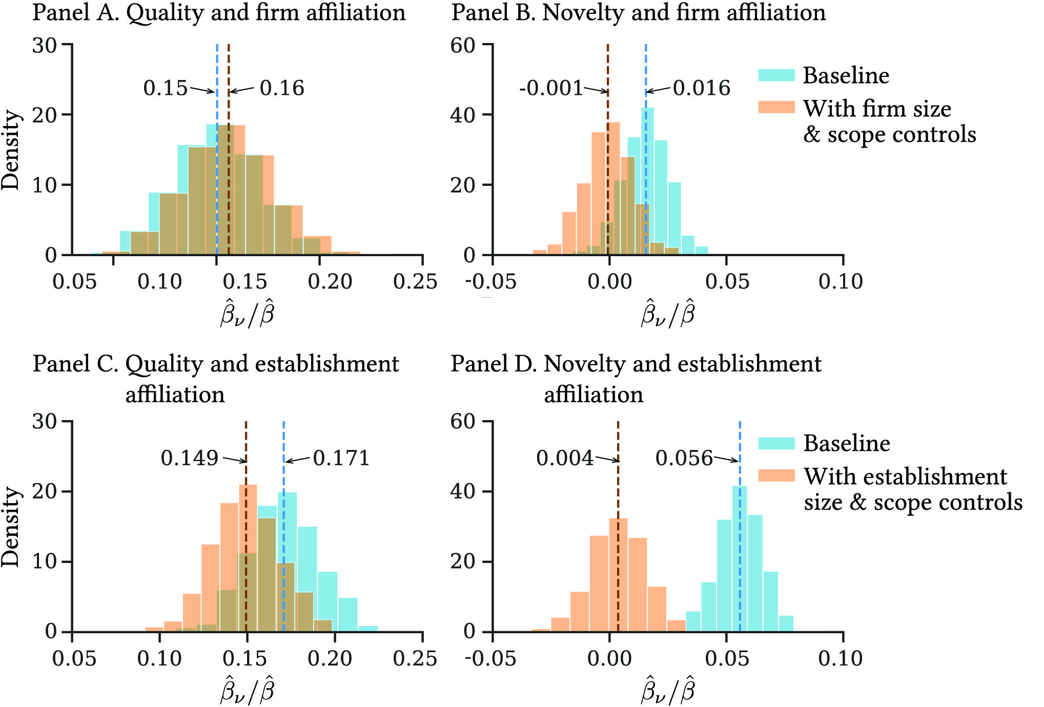 Figure 7
 Figure 8
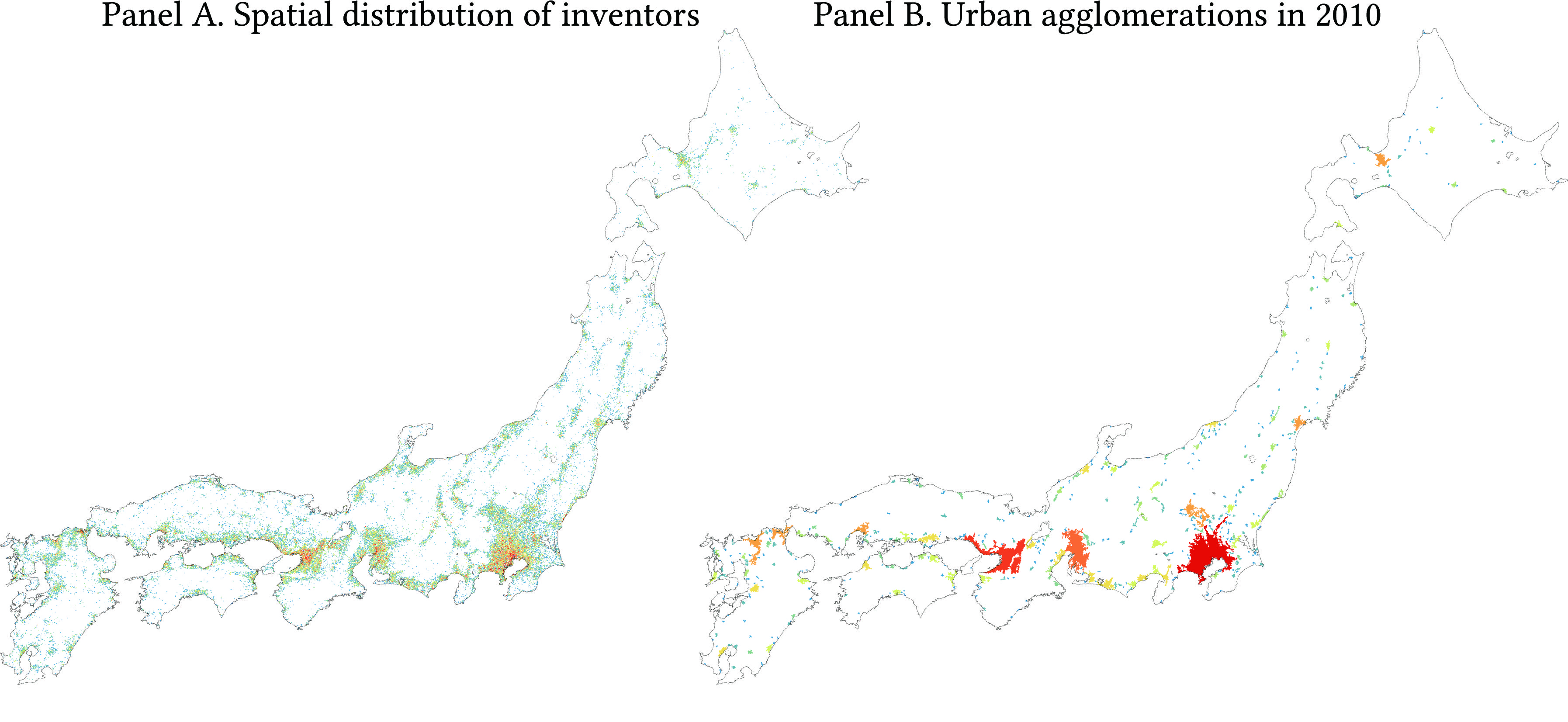 Figure 9
| Panel A. Quality | |||||
| Variable | (1) OLS | (2) IV3-5 | (3) IV3 | (4) IV4 | (5) IV5 |
| 0.166 | 0.334 | 0.340 | 0.392 | 0.488 | |
| (0.0111) | (0.0444) | (0.0440) | (0.0565) | (0.118) | |
| 0.163 | 0.140 | 0.139 | 0.132 | 0.119 | |
| (0.0326) | (0.0213) | (0.0212) | (0.0199) | (0.0192) | |
| -0.0744 | -0.0669 | -0.0666 | -0.0643 | -0.0600 | |
| (0.0116) | (0.00818) | (0.00816) | (0.00765) | (0.00721) | |
| 0.123 | 0.106 | 0.104 | 0.091 | 0.059 | |
| 52.96 | 179 | 41.90 | 8.413 | ||
| Critical -value | 20.09 | 23.11 | 23.11 | 23.11 | |
| Hansen -value | 0.681 | ||||
| Panel B. Novelty | |||||
| Variable | (1) OLS | (2) IV3-5 | (3) IV3 | (4) IV4 | (5) IV5 |
| 0.217 | 0.480 | 0.478 | 0.511 | 0.495 | |
| (0.00693) | (0.0403) | (0.0409) | (0.0335) | (0.0491) | |
| 0.235 | 0.189 | 0.190 | 0.184 | 0.187 | |
| (0.0187) | (0.0166) | (0.0166) | (0.0174) | (0.0202) | |
| -0.182 | -0.161 | -0.161 | -0.158 | -0.160 | |
| (0.0148) | (0.00924) | (0.00920) | (0.00982) | (0.00916) | |
| 0.175 | 0.134 | 0.135 | 0.124 | 0.129 | |
| 332.9 | 1009 | 720.8 | 166.3 | ||
| Critical -value | 17.85 | 23.11 | 23.11 | 23.11 | |
| Hansen -value | 0.113 | ||||
Peer Reviews
No public reviews on file for this paper yet. If you reviewed it on a platform where reviews are public (OpenReview, ICLR, NeurIPS, ICML), you can paste yours below so the community can read it here.
Videos
No videos yet. Explain this paper in a talk, walkthrough, or lecture? Add one.
Taxonomy
TopicsFirm Innovation and Growth · Intellectual Property and Patents · Innovation Policy and R&D
\draftSpacing
1.5
\shortTitle\pubMonth\pubYear\pubVolume\pubIssue\JEL
D83, D85, O31, R11, C33, C36 \KeywordsKnowledge creation, Collaboration, Differentiated knowledge, Patents, Technological novelty, Network
Creation of Knowledge through Exchanges of Knowledge: Evidence from Japanese Patent Data
Tomoya Mori and Shosei Sakaguchi Mori: Corresponding author. Institute of Economic Research, Kyoto University, Yoshida-Honmachi, Sakyo-Ku, Kyoto 606-8501, Japan, [email protected]; Research Institute of Economy, Trade and Industry, 11th floor, Annex, Ministry of Economy, Trade and Industry, 1-3-1 Kasumigaseki Chiyoda-Ku, Tokyo 100-8901, Japan. Sakaguchi: Department of Economics, University College London, Gower Street, London WC1E 6BT, UK, [email protected]. Acknowledgements: Earlier versions of this paper were presented at Jinan University, Keio University, Kyoto University, RIETI, the University of Tokyo, the 32nd ARSC meeting at Nansan University, the 13th UEA meeting at Columbia University, the 2nd CURE meeting at Singapore Management University, and the Workshop on Innovation, Technological Change, and International Trade at the Technical University of Munich. The authors are particularly indebted to Marcus Berliant, Jorge De la Roca, Gilles Duranton, Masahisa Fujita, Tadao Hoshino, Wen-Tai Hsu, Daishoku Kanehara, Shin Kanaya, Kentaro Nakajima, Ryo Nakajima, Yoshihiko Nishiyama, Ryo Okui, Akihisa Shibata, and Jens Wrona for their constructive comments. This research was conducted as part of the project “An empirical framework for studying spatial patterns and causal relationships of economic agglomeration” undertaken at RIETI. It received partial financial support from JSPS Grants-in-Aid for Scientific Research grant numbers 15H03344, 16K13360, and 17H00987.
(March 2, 2024)
Abstract
This study shows evidence for collaborative knowledge creation among individual researchers through direct exchanges of their mutual differentiated knowledge. Using patent application data from Japan, the collaborative output is evaluated according to the quality and novelty of the developed patents, which are measured in terms of forward citations and the order of application within their primary technological category, respectively. Knowledge exchange is shown to raise collaborative productivity more through the extensive margin (i.e., the number of patents developed) in the quality dimension, whereas it does so more through the intensive margin in the novelty dimension (i.e., novelty of each patent).
Knowledge is a key element in various aspects of economic modeling. The theoretical development of innovation-driven economic growth dates back at least to [37, 36] and [34, 16, 1]. Formalization has focused on different aspects of knowledge, such as the tension between learning-by-doing and innovation [[, e.g.,]]Klette-Kortum-JPE2004, spillovers [[, e.g.,]]Jovanovic-Rob-REStud1989, and imitations [[, e.g.,]]Perla-Tonetti-JPE2014. Some have described the mechanism of knowledge creation. In [41], extant ideas induce the development of new ideas if recombined with other existing ideas. [30, 31] formalized the recombination of ideas by their convex combinations. [2] considered team formation by endogenous specialization between a leader and members of a team from ex ante symmetric agents.
This study focuses on the theory of [6] with regards to the mechanism of collaborative knowledge creation. What facilitates collaboration is the exchange of mutual differentiated knowledge between collaborators through their common knowledge. The key mechanics underlying their theory is that the relative size of common and differentiated knowledge varies depending on the duration of collaboration. A longer duration of collaboration increases common knowledge whereas it decreases differentiated knowledge between collaborators, while the opposite is true between non-collaborators. To maintain balance between the two types of knowledge with their collaborators, inventors seek polyadic collaborations and rotate their collaborators.
Extant empirical studies have primarily focused on knowledge spillovers associated with R&D expenditure or transactions by firms and industries [[, e.g.,]]Griliches-BJ1979,Scherer-REStat1982,Jaffe-AER1986, or through flows of patent citations [[, e.g.,]]Jaffe-et-al-AER2000. Recent studies have explored more specific channels of knowledge spillovers. For example, [7] distinguished positive effects of R&D spillover from negative ones in sharing product markets between firms. [42] proposed a microeconomic model and showed evidence for knowledge spillover among firms through inventor networks. Other studies have utilized exogenous termination of collaborations for the identification of peer effects [[, e.g.,]]Waldinger-JPE2010 and positive externality from superstars in research [[, e.g.,]]Azoulay-et-al-QJE2010.
Using patent data from Japan, this study contributes to the niche empirical literature by showing evidence for collaborative knowledge creation through active exchanges of knowledge among individual inventors, rather than passive improvement of productivity via spillovers. Based on [6], our baseline regression model focuses on an inventor and their average collaborator. It expresses the causality between their pairwise collaborative productivity and the differentiated knowledge of the average collaborator. Collaborative output is measured in terms of quality and novelty of patents. For a given patent, the quality is evaluated by forward citations, and the novelty by the order of application within their primary technological category, reflecting the scarcity of invention in this category.
In this regression, we control for individual fixed effects by exploiting panel data and a variety of other factors. However, we face identification problems due to the remaining unobserved factors that influence inventors’ collaboration and knowledge creation. To deal with an endogenous regressor for an inventor (i.e., the differentiated knowledge of collaborators), we propose instrumental variables constructed from the same endogenous variables of their distant indirect collaborators. Using more distant indirect collaborators to construct instrumental variables, one can reduce endogeneity caused by unobserved factors [[, e.g.,]]Zacchia-REStud2020 and by reflection problems [[, e.g.,]]Bramoulle-et-al-JE2009, although this also makes the instruments weaker. However, we argue that there is a channel in which our instruments retain relevance through firm-specific factors while maintaining their exogeneity.
Our baseline results indicate that a 10% increase in collaborators’ differentiated knowledge for an inventor raises the quality and novelty of their average pairwise output by 3%–4% and 5%, respectively. Moreover, we found that in the contribution of knowledge exchange to the quality and novelty of collaborative output, 17% and 65% can be attributed to the intensive margin (i.e., the average quality and novelty of output, respectively), rather than to the extensive margin (i.e., the number of patents developed). Thus, collaborations appear to be more effective for seeking novelty of output.
The remainder of this paper is structured as follows. Section 1 introduces the model by [6], and Section 2 explains the motivating fact. Section 3 describes the data, Section 4 details the regression models, and Section 5 discusses our identification strategy. Section 6 presents the empirical results. Finally, Section 7 concludes the paper.
1 A Mechanism of Collaborative Knowledge Creation
Here, we describe the Berliant-Fujita (BF) model. Each agent develops new knowledge either in isolation or by collaborating in pairs, building on their accumulated stock of knowledge. Consider a given set of agents who engage in knowledge creation. They are assumed to be a priori homogeneous but become heterogeneous in the composition of the set of knowledge they created in the past. Let be the proportion of time that agent allocates for collaboration with . If agent works in isolation, then their knowledge creation is subject to constant returns technology as given by if and 0 otherwise, where , is the knowledge stock of agent , and is the output.
If the subject instead collaborates with agent , then their joint output is given by
[TABLE]
for and otherwise, where , is the common knowledge of and ; is the knowledge of agent differentiated from that of ; and is the relative importance of common knowledge. All pieces of knowledge (irrespective of timing at which they are created) are horizontally and symmetrically different.111The BF model of knowledge creation by exchanging mutual differentiated knowledge is consistent with the knowledge creation by recombination considered by [41] and [30, 31].
The output from the collaboration of agents and becomes their common knowledge. Thus, the common knowledge of and increases as their collaboration lasts longer, and at the same time the differentiated knowledge between with agents other than also increases relative to their common knowledge. To achieve the best balance between common and differentiated knowledge with collaborators, agents collectively decide on the group of collaborators, where each agent optimally chooses for each of their collaborators to maximize the total output (assuming an equal split of output between collaborators).
Agents are assumed to maximize the present value of their lifetime knowledge production. In a typical steady-state equilibrium, the size of the network component of each agent is given by .222Myopic core is adopted as the equilibrium concept. A typical steady-state equilibrium is the one resulting from the initial state in which agents have sufficient common knowledge for the starting collaboration. Agents continue to rotate their collaborators so that the share of the total time is allocated to each pairwise collaboration [[]Proposition 1]Berliant-Fujita-IER2008.
While the model is highly stylized, it formalizes a microeconomic mechanism in which explicit knowledge exchange induces the creation of new knowledge.
2 A Motivating Fact
Here, we define the key variables and present a motivating fact for our study. We use patent application data from Japan and construct two-period balanced panel data by aggregating five consecutive years from 2000 to 2004 and from 2005 to 2009 to form periods 1 and 2, respectively.
Consider patent development in period by the set of inventors in the panel and their collaborators. Let be the set of patents in which inventor participates in the development, and for is the set of inventors who participate in patent . Denoting the value of patent by a scalar , the productivity of inventor is defined in terms of the total value of patents in which they participated, with the value of each patent being discounted by the number of inventors involved in the patent:
[TABLE]
where is the cardinality of set . Hereafter, the expression for a set denotes the cardinality of . Let
[TABLE]
represent the set of collaborators of inventor such that each agent in participates in at least one common patent with in period . Then,
[TABLE]
represents the average pairwise output by inventor in period , where is the total number of collaborators of in period . It can be interpreted as the collaborative output of inventor with their average collaborator, corresponding to in (1).
We focus on the role of knowledge exchange in the BF model, and hence the differentiated knowledge of collaborators in (1). To simplify the analysis, we assume that the cumulative knowledge of an inventor is fully utilized in the knowledge creation in each period, and hence it is reflected in their output in the same period. Accordingly, the average differentiated knowledge of collaborators of inventor in period is assumed to be reflected in the average output that the collaborators of produced outside the joint projects with in the same period:
[TABLE]
Turning to the quantification of collaborative productivity, we consider the quality and novelty dimensions. The quality of a patent is measured by cited counts. Specifically, represents the count of citations that patent received in five years after publication. Here, excludes citations from the patents in which any firm employing the inventors in is involved.333More precisely, let period 3 include all years from 2010, and let be the set of all patents applied in periods and . Let be the set of inventors who belong to the same firm as inventor in period . Then, the set of potential citing patents for patent is given by . Note that our quality-measure is far more conservative than a simple exclusion of self-citation at the inventor or firm level. This construction eliminates obvious correlations between and due to mutual citations among the firms affiliating in R&D.
The novelty of a patent, on the other hand, is measured in terms of the scarcity of existing patents sharing the same technological category with the patent. Specifically, is defined by the reciprocal, , of the order, , of with respect to its application date among all the patents classified in the same technological category as . In our analysis, the technological category adopted to compute the patent novelty is a ‘subgroup’ of the International Patent Classification (IPC) and is the most disaggregated technological category available in the data. There were 31,511 and 26,424 subgroups with positive numbers of patents applied in periods 1 and 2, respectively.444Refer to Appendix LABEL:app:data (Table LABEL:tb:descriptive-stat) as well as Appendix LABEL:app:ipc for more details on technological categories in IPC.
Alternatively, the novelty of a patent has been defined, for example, by [13] to be the number of new subclass pairs associated with the patent.555They used the United States Patent Classification with 10,000 subclasses. However, this measure is too extreme for our purpose, since a patent’s novelty is zero unless it has at least a new subclass combination. A recent measure of novelty by [40] is based on the frequency of word combinations appearing in the text of a patent in older patents. It may capture some aspects that are missed in our definition of novelty, and vice versa. However, the correspondence between arbitrary word combinations and technologies is not clear at this point. We thus adopt a novelty measure that is consistent with the technological categories of IPC, which defines the similarity and dissimilarity of all the patents in our data.
Figure 1 shows the relation between and in period 1. Panels A and B indicate a clear positive relationship between the two variables under quality and novelty measures, respectively. In particular, for the quality-based productivity in Panel A, by construction, the positive correlation does not accrue from mutual citations among collaborators or their employer firms. This provides us a motivating fact for investigating the causal effect suggested by the BF model.
3 Data
Patent data – Patent data are taken from the published patent applications of Japan [[]]Naito-Data, including information on all patents applied for between 1993 and 2017. Since every applied patent is published within 1.5 years of application, our data include all the output of inventors at a given point in time during the study period.
In this data, identical inventors are traced by matching their names and the establishments they belong to, recorded in the applications of patents in which they participated. By utilizing this information, we focus on the panel of inventors constituting set who had been active and stayed in the same establishments (and hence the same firms) in both periods, and they have up to the 5th indirect collaborators in each period. This panel helps us to isolate inventor and firm-specific factors that may influence knowledge creation. The indirect collaborators are used to construct instrumental variables in order to eliminate influence from other endogenous factors. Descriptive statistics of the data concerning the inventors in are shown in Appendix LABEL:app:data.
The information on inventors not included in is still used if they either directly or indirectly collaborate with inventors in . Specifically, there are 434,555 and 283,860 direct and indirect collaborators in total in periods 1 and 2, respectively. The inventors in for regressions account for only 6.7% and 8.8% of all the inventors with at least one collaborator in periods 1 and 2, respectively. Nonetheless, neither the quality nor novelty of the developed patents exhibit stark differences between the two sets of inventors. For the average quality (novelty) of patents in pairwise collaborative output, in period 1, the mean values are -3.95 and -3.02 (-8.82 and -8.61) with standard deviations of 1.77 and 1.97 (2.01 and 2.61) for inventors in and for the full samples, respectively (Figure LABEL:fig:productivity_dist in Appendix LABEL:app:data compares their distributions between the selected and full samples).
Each patent is associated with at least one technological classification based on the IPC, which is maintained by the World Intellectual Property Organization (http://www.wipo.int/portal/en/index.html). The IPC hierarchically classifies technologies into eight sections, 120 classes, 300 subclasses, and finally 40,000 subgroups. The IPC’s labeling scheme is consistent over time, and a newly introduced category is basically associated with a new technology. Hence, the classifications in IPC at a given point in time roughly represent the state-of-the-art technological categories at that time.666See Appendix LABEL:app:ipc for the details of the IPC technological categories. Although an applicant can claim more than one IPC category for their patent, we adopted only the primary IPC category of each patent to represent its technological category to avoid subjective variation. We adopt the finest subgroup classification to define the novelty of the patents, which together comprise 40,691 and 38,339 categories associated with the patents in our data in periods 1 and 2, respectively.
Urban agglomerations – R&D activities are disproportionately concentrated in large cities (see Figure LABEL:fig:ua in Appendix LABEL:app:locational-factors). If an urban agglomeration (UA) is defined as a contiguous area of population density of at least 1000/km2 and with a total population of at least 10,000,777Population data are obtained from the Population Census (28) by MIAC. in 2000, 99% of all inventors concentrated in UAs, with 81% in the largest three UAs. Inventors located within a 10 km buffer of any of the 453 UAs are assigned to the closest UA; otherwise, their locations are considered to be rural. In the regressions, the standard errors are clustered by UAs.888As UAs spatially expand over time on average, we use the boundaries of UAs in 2010, each of which provides the largest spatial extent during the study period 1995–2009 on average. However, the choice of the particular time point should not affect the basic results because most inventors are concentrated in relatively large UAs whose spatial coverage is relatively stable over the study period.
Geographic neighborhood factors – Given the disproportionate geographic concentration of R&D activities, productivity is expected to be influenced by geographic neighborhood [[, e.g.,]]Jaffe-Trajtenberg-Henderson-QJE1993,Thompson-Fox-Kean-2005,Kerr-Kominers-REStat2015. We control for the geographic concentrations of five types of activities: inventors, R&D expenditure, manufacturing employment and output, and residential population. Each geographic concentration is defined by the size of the concentration in a circle of given radius around inventor . The formal definitions and descriptive statistics are described in Appendix LABEL:app:locational-factors.
4 Regression Models
Here, we describe the regression models. We focus on collaborative cases and do not address the possibility of working in isolation. To apply data to theory, the original specification is simplified by formulating a regression model for knowledge creation between an inventor and their average collaborator rather than between each pair of inventors:
[TABLE]
In the theoretical model, we focus on knowledge exchange, and hence the role of the differentiated knowledge of collaborators in (1), while abstracting from the role of common knowledge and differentiated knowledge of inventor . The effect of knowledge exchange should naturally be reflected in that of the average differentiated knowledge of collaborators, in (6).
To control for other non-negligible knowledge effects, we include the cumulative research scope of inventor s’ past projects. For this purpose, let denote the set of all technological categories (i.e., IPC subgroups), and the technological category assigned to patent be . Then, the research scope of inventor in period is defined by
[TABLE]
which in turn can be used to define the cumulative research scope of inventor in period by999To compute for , we use all available data from 1993. Specifically, we define period 0 to be from 1993 to 1999.
[TABLE]
The past experience of inventor reflected in this value is naturally expected to correlate with the size of common knowledge between inventor and their collaborators as well as the differentiated knowledge of . In addition, it may partly control for other factors discussed in the literature; for example, technological obsolescence [[, e.g.,]]Horii-JEDC2012, imitations [[, e.g.,]]Chu-JEG2009,Cozzi-Galli-JEG2014, and learning-by-doing effects [[, e.g.,]]Grossman-Helpman-Book1991,Klette-Kortum-JPE2004, Lucas-Moll-JPE2014. The third and fourth terms on the RHS of (6) are supposed to capture their overall effects up to the second order.
Other inventor- and time-specific productivity shifters for inventor are bundled in the fifth term, . Namely, represents a vector of geographic neighborhood effects defined in Section 3 that includes local concentrations of other inventors, R&D expenditure, manufacturing employment/production, and residential population; is a vector of coefficients corresponding to each element of . The last three terms, , , and , on the RHS are the time-invariant inventor fixed effect, period fixed effect, and inventor- and period-specific error, respectively. The values of parameters , and are estimated by regressions.
Note that the technology of knowledge creation (1) itself, and hence the corresponding empirical model (6), is not restricted to any specific mechanism of inventors’ collaboration, although the BF model assumes autonomous collaborations by inventors. Consequently, in (6) it does not matter for parameter identification whether network formation is autonomous or determined at the firm or establishment level.
Finally, we exploit the log-linear relation between quantity and quality (or novelty) of collaborative productivity given by (2):
[TABLE]
In the first term on the RHS of (9), denotes the number of patents included (i.e., the extensive margin) in inventor ’s pairwise output given by , where , which coincides with under in (2). In the second term, represents the average quality or novelty (i.e., the intensive margin) of ’s pairwise output, . We can thus decompose the effect of each explanatory variable in (6) into those related to the quantity and average quality/novelty of inventors’ pairwise output . The model to be estimated for this purpose is given by
[TABLE]
for , where the coefficients of each explanatory variable for add up to that of the corresponding variable in (6). In particular, we have for the coefficient of .
5 Identification by Instrumental Variables
Here, we present our strategy for model identification by dealing with the endogeneity of the average differentiated knowledge of collaborators in (6). There are three sources of endogeneity. The first results from inventors’ endogenous collaboration; that is, network endogeneity, where unobservable influences exist on inventors’ collaboration decisions and their productivities [[, e.g.,]]Goldsmith-Pinkham-Imbens-JBES2013. The second results from the mutual dependence of productivities between an inventor and their collaborators through in (6). This is the so-called ‘reflection problem’ in the context of econometric network analysis [[, e.g.,]]Manski-REStud1993, Bramoulle-et-al-JE2009. The third arises from unobservable network specific factors that influence an inventor and their collaborators’ productivities simultaneously. These are called ‘correlated effects’ in [27]. To solve the endogeneity caused by these reasons, we argue that the endogenous variables in (6) for inventor can be instrumented by the average value of the same variable for the distant indirect collaborators of .
Let be the set of all the 0-th to -th indirect collaborators of inventor given by
[TABLE]
where the set of the ‘0-th indirect collaborators’ is defined by the set of inventors comprising and their direct collaborators . To obtain from for , we expand by the union of all the direct collaborators of as in (11). The set of the -th indirect collaborators of can then be given by
[TABLE]
The instrument for can be constructed as the average values of the differentiated knowledge of collaborators for -th indirect collaborators :
[TABLE]
where .
Exogeneity of the instruments – The extant literature on social interactions [[, e.g.,]]Bramoulle-et-al-JE2009, De-Giorgi-et-al-AEJ2010, Calvo-Armengol-et-al-REStud2009 suggests that the reflection problem in our context be reduced by using instruments constructed from indirect collaborators. Namely, the farther an indirect collaborator is from an inventor in the collaboration network, the smaller the influence of their output on the inventor’s productivity.101010For example, in eq. (6) of [8], the endogenous peer effect from the -th indirect peer is given by , where and with the [math]-th indirect peer being the direct peer. The peer effect from the -th indirect peers diminishes as increases. The instruments further solve the endogeneity caused by the endogenous network and correlated effects, if more distant inventors share less unobserved factors.
This effect applies to our case if, for example, inventors with similar (observable and unobservable) characteristics have proclivities to collaborate with each other. An obvious situation is that inventors belong to the same firm. However, this case is not an issue for us, since firm-specific factors can be controlled by inventor fixed effects. Another typical situation is that inventors have similar technological specializations. These inventors likely share opportunities to exchange ideas with each other through, for example, conferences and journals of common research subjects, thereby affecting their chance of collaboration and productivities. The exogeneity of the instruments in this case arises from the fact that more distant indirect collaborators share less common research fields with each other.111111Our logic for the exogeneity of the instruments is similar to that of [42], who used similar instruments to identify knowledge spillovers between firms through their inventor networks.
To see if our data supports this conjecture, we quantify the commonality in technological specialization between indirect collaborators using the Jaccar index. The average Jaccar index between the technological specialization of inventor and those of their -th indirect collaborators is computed as:
[TABLE]
A larger value of implies higher average similarity in technological specialization between inventor and their -th indirect collaborators. In particular, it takes value 0 if their specializations do not overlap (i.e., ) and value 1 if they are identical (i.e., ).
In Figure 2, Panel A depicts the average values of overall in terms of IPC sections, classes, subclasses, and subgroups between an inventor and their -th indirect collaborators for . Panel B complements it by showing the average count of common technological categories in the corresponding classifications between an inventor and their -th indirect collaborators. From Panel A, the commonality of specializations steadily decreases as the indirectness increases. In terms of the IPC subgroup, it almost vanishes for the 3rd indirect collaborators. In terms of the average count of common categories, it is less than 1 for the 3rd and higher indirect collaborators for all classifications in IPC.
Relevance of instruments – Suppose that endogeneity is partly caused by some time-invariant unobserved factors specific to the firms or establishments that inventors belong to. In this situation, there is a possible channel over the collaboration network through which our instruments retain relevance while satisfying exogeneity. We elaborate a simple example here. Note that the set of collaborators and the set of -th indirect collaborators of inventor may contain inventors that belong to the same firms, but which are different from the one belongs to. For these inventors, the productivities, and hence and , correlate through the firm-specific factors.121212Alternatively, and also correlate if the 1st-indirect and -th indirect collaborators of belong to the same firm. On the other hand, they do not have common firm-specific factors with . Consequently, there is no correlation between and through unobserved factors.131313Although possibly contains inventors that belong to the same firms as , their common firm-specific factors are controlled by inventor ’s fixed effect and hence do not violate the exogeneity condition.
Whether there is sufficiently strong relevance of instruments is an empirical question to be examined in Section 6. The success in our case hinges on the fact that a relatively large share of distant indirect collaborators belong to the same firms. Specifically, the shares of the 3rd, 4th, and 5th-indirect collaborators of an inventor who belong to the same firm as the inventor are 50%, 38%, and 25% (54%, 43%, and 32%) on average, respectively, in period 1 (period 2).
6 Results
Here, we present our main regression results for models (6) and (10) with brief discussions on robustness checks, the details of which are given in Appendix LABEL:app:robustness. In all of the regressions conducted, the fixed effects of inventors, periods, and IPC classes are controlled. The geographic neighborhood factors described in Section 3 are constructed for a circle with a 1 km radius around each inventor except for residential population, which is computed within a 20 km radius around an inventor to account for the urban environment around them. Standard errors are clustered by UAs (see Section 3).141414As the instruments for in (6) and (10) involve inventors located in different UAs, one might suspect that cluster-robust standard errors are incorrect because the instruments for any inventor might be correlated with errors in (6) for any inventor even if inventors and are located in different UAs. However, we consider that these cluster-robust standard errors still provide correct standard errors because the inventor fixed effects controlled in all regressions encompass UA-specific fixed effects, making the errors free from correlation with UAs while allowing for standard errors to vary across UAs.
Baseline results – Panels A and B in Table 1 summarize the regression results for key variables of model (6) under quality- and novelty-adjusted productivity, respectively. More detailed tables with estimated coefficients for neighborhood factors are described in Appendix LABEL:app:baseine (Tables LABEL:tb:bf-model-citation-full-result and LABEL:tb:bf-model-novelty-full-result).151515The estimated coefficients of the key variables in Table 1 change only marginally under alternative radius values (5 and 10 km) adopted to compute geographic neighborhood factors. In both panels, column 1 reports the result from the OLS regression, and the rest report those from two-stage least squares (2SLS) instrumental variable (IV) regressions. For the IV regressions, we use the 3rd to the 5th indirect collaborators to construct IVs for . More specifically, we use all three instruments for and in column 2, while only one is used in columns 3–5, respectively.
The IV results support the role of knowledge exchange in the BF model. The estimated coefficients of are persistently positive and similar, 0.33–0.39 and 0.48–0.51, for quality- and novelty-based productivity, respectively (except for the IV5-result in Panel A, which is discussed later). The values below 1 indicate decreasing returns to knowledge exchange, which is consistent with the implication of the BF model that the benefit from collaborators’ differentiated knowledge will eventually be dominated by that of common knowledge with collaborators and the inventors’ own differentiated knowledge.
The estimated positive effect of research scope of an inventor and the negative effect of its squared term are consistent with the interpretation of positive decreasing-returns effects of common knowledge as well as differentiated knowledge of the focal inventor, together with other possible effects such as learning-by-doing effects discussed in Section 4.
To examine the strength of instruments, we conducted the heteroskedasticity robust weak instrument test of [53]. Except for the IV regression based on the 5th indirect collaborators for the quality-based case (column 5 in Panel A), [53]’s first-stage effective statistics, , take large values, meaning that the IVs do not seem to be weak.161616See Table LABEL:tb:first-stage in Appendix LABEL:app:baseine for the results of the first-stage regressions. Indeed, the estimated coefficient of in column 5 in Panel A (which is instrumented by ) seems to differ from the others. To confirm the exogeneity of the IVs, we use for all and in column 2 and conduct Hansen’s (\citeyearHansen-ECTA1982) test for overidentifying restrictions. The p-values of the test are 0.68 and 0.11 for productivities based on quality and novelty, respectively, meaning that the exogeneity of the IVs cannot be rejected.171717Of course, this result of Hansen’s test is by no means sufficient to guarantee the exogeneity of the instruments if all the instruments are subject to the same type and magnitude of bias.
The OLS result is consistent with the IV results in terms of the signs of the estimated coefficients, but it appears to have a substantial downward bias in the estimated coefficient of under both measures of productivity.181818[2] and [42] reported similar downward bias on the effects of spillovers/interactions from other agents on the R&D outcome. A possible explanation for the bias is that the more productive inventors attract (or are assigned by their firm) a larger number of relatively unexperienced collaborators than the inventor intends. The removal of this reverse causality leads to a larger positive effect in the IV estimates.
Robustness checks – The estimated coefficient of in (6) might reflect not only the effects of differentiated knowledge of collaborators, but also those of time-varying factors specific to the inventors’ own and collaborators’ firms or establishments. Such factors include the R&D environment and productivity externality (peer effects) from (possibly non-collaborating) inventors that vary across firms or establishments, and their research affiliations.
To investigate these possibilities, we conduct the two exercises (see Appendix LABEL:app:robustness for details). First, we include the size and research scope of the firm or establishment to which an inventor belongs as additional explanatory variables in (6). Second, we consider possible influences from the broader neighborhood in the research network beyond an inventor’s own firm or establishment. Specifically, we simulate random counterfactual choices of collaborators for each inventor in conditional on the actual number of collaborators as well as the firms/establishments to which these collaborators belong. We then replace in (6) with that constructed from the counterfactual collaborators and estimate the model. We find that the effect of knowledge exchange on the collaborative productivity appears to be at most mildly influenced by factors at the level of an establishment, a firm, and a research affiliation of firms or establishments.
Quantity–quality/novelty decomposition – Finally, we turn to the quantity-quality/novelty decomposition of the effect of knowledge exchange on collaborative output based on (9) and (10). Figure 3 shows the point estimate and 95% confidence intervals of the estimated shares, , of contributions accruing from knowledge exchange on the average quality and novelty of output.191919For each , the estimate and confidence interval of are calculated by the generalized method of moments, which simultaneously estimates the baseline model (6) and the decomposed model (10) with the 2SLS weighting matrix. The comprehensive regression results are relegated to Appendix LABEL:app:qq (Tables LABEL:tb:qq-decomposition-citation and LABEL:tb:qq-decomposition-novelty). The first stage of the regression is shared with (6) and presented in Appendix LABEL:app:baseine (Table LABEL:tb:first-stage).
We find contrasting roles of knowledge exchange between the quality and novelty of output: % of its contribution can be attributed to increasing the quantity rather than the quality of research output under the quality-adjusted productivity measure, whereas 65% of the contribution accrues to increasing the average novelty rather than quantity of research output under the novelty-adjusted measure. The result indicates that knowledge exchange is comparably more effective for seeking technological novelty than it is for increasing the quality of research output.
Our findings agree with the results of [13] in that cohesiveness of a researcher network has negative effects on the novelty of their developed patents. Since the cohesiveness is expected to be positively correlated with the amount of common knowledge between collaborators, a larger cohesiveness may imply smaller differentiated knowledge within the researcher network, and hence less novelty of output.
7 Conclusions
We have shown evidence consistent with the collaborative knowledge creation mechanism proposed by [6]. To our knowledge, our work is the first to provide micro-econometric evidence for collaborative knowledge creation through the exchange of knowledge at the individual inventor level. We also found that knowledge exchange tends to raise the novelty comparably more than the quality of collaborative invention.
This evidence has important policy implications. Namely, firms, cities, regions, and countries that promote encounters and collaboration among inventors across organizations and institutions, despite the possibility of imitations and undesired diffusion, may have better chances to foster innovation through knowledge exchange.
In the future, it will be of interest to further investigate the roles of firms in R&D. As financial resources for R&D are typically provided by firms, firm-specific patterns of collaborations and R&D policies could affect the productivity of individual inventors and firms.202020See [3] for an initial attempt in this direction as they distinguish between R&D that is internal and external to firms and study the firm dynamics that arise from this distinction. By matching the addresses of establishments in the patent database with those of the Census of Manufacturers, it is also possible to investigate the impact of patent development on firm productivity. Second, non-technological diversity of collaborators in terms of, for example, gender, age, and cultural background, may affect productivity. For example, [32] and [19] found a positive influence of gender diversity on innovation of Danish and Japanese firms, respectively.
References
- [43] Lars Peter Hansen
“Large sample properties of generalized method of moments estimators”
In Econometrica 50.4, 1982, pp. 1029–1054
- [44] Adam B. Jaffe, Manuel Trajtenberg and Rebecca Henderson
“Geographic localization of knowledge spillovers as evidenced by patent citations”
In The Quarterly Journal of Economics 108.3, 1993, pp. 577–598
- [45] William R. Kerr and Scott Duke Kominers
“Agglomerative forces and cluster shapes”
In Review of Economics and Statistics 97.4, 2015, pp. 877–899
- [46] Ministry of Economy, Trade and Industry of Japan
“Census of Manufactures”, 2000, 2005
- [47] Ministry of Economy, Trade and Industry of Japan
“METI Basic Survey of Japanese Business Structure and Activities”, 2000-2010
- [48] Ministry of Internal Affairs and Communications of Japan
“Economic Census for Business Frame”, 2009
- [49] Ministry of Internal Affairs and Communications of Japan
“Establishment and Enterprise Census”, 2001, 2006
- [50] Ministry of Internal Affairs and Communications of Japan
“Population Census (Tabulation for standard area mesh)”, 2000, 2005
- [51] Ministry of Internal Affairs and Communications of Japan
“Survey of Research and Development”, 2000-2010
- [52] Yasusada Murata, Ryo Nakajima, Ryosuke Okamoto and Ryuichi Tamura
“Localized knowledge spillovers and patent citations: A distanced-based approach”
In Review of Economics and Statistics 96.5, 2014, pp. 967–985
- [53] José Luis Motiel Olea and Carolin Pflueger
“A robust test for weak instruments”
In Journal of Business & Economic Statistics 31.3, 2013, pp. 358–369
- [54] Peter Thompson and Melanie Fox-Kean
“Patent citations and the geography of knowledge spillovers: A reassessment”
In The American Economic Review 95.1, 2005, pp. 450–460
APPENDICES
knowledge_appendix.tex
The reference list from the paper itself. Each links out to its DOI / PubMed record.
- 1[1] Philippe Aghion and Peter Howitt “A model of growth through creative destruction” In Econometrica 60.2 , 1992, pp. 323–351
- 2[2] Ufuk Akcigit, Santiago Caicedo, Ernest Miguelez, Stefanie Santcheva and Valerio Sterzi “Dancing with the stars: Innovation through interactions” Discussion paper No. 24466, National Bureau of Economic Research, 2018
- 3[3] Ufuk Akcigit and William R. Kerr “Growth through heterogeneous innovations” In Journal of Political Economy 126.4 , 2018, pp. 1374–1443
- 4[4] Artificial Life Laboratory, Inc. “Patent database for research”, 2018
- 5[5] Pierre Azoulay, Joshua S. Zivin and Jialan Wang “Superstar extinction” In The Quarterly Journal of Economics 125.2 , 2010, pp. 549–589
- 6[6] Marcus Berliant and Masahisa Fujita “Knowledge creation as a square danc on the Hilbert cube” In International Economic Review 49.4 , 2008, pp. 1251–1295
- 7[7] Nicholas Bloom, Mark Schankerman and John Van Reenen “Identifying technology spillovers and product market rivalry” In Econometrica 81.4 , 2013, pp. 1347–1393
- 8[8] Yann Bramoullé, Habiba Djebbari and Bernard Fortin “Identification of peer effects through social networks” In Journal of Econometrics 150.1 , 2009, pp. 41–55