Faster Guarantees of Evolutionary Algorithms for Maximization of Monotone Submodular Functions
Victoria G. Crawford

TL;DR
This paper introduces new evolutionary algorithms with improved theoretical guarantees for maximizing monotone submodular functions under cardinality constraints, achieving near-optimal ratios with fewer function queries.
Contribution
The paper proposes a novel Pareto optimization algorithm and a biased Pareto optimization variant with improved query complexity and approximation guarantees for submodular maximization.
Findings
Algorithms achieve a $(1- rac{1}{e})$ approximation ratio in expectation.
The algorithms require fewer function evaluations compared to existing methods.
Empirical results support the theoretical improvements over stochastic greedy algorithms.
Abstract
In this paper, the monotone submodular maximization problem (SM) is studied. SM is to find a subset of size from a universe of size that maximizes a monotone submodular objective function . We show using a novel analysis that the Pareto optimization algorithm achieves a worst-case ratio of in expectation for every cardinality constraint , where is an input, in queries of . In addition, a novel evolutionary algorithm called the biased Pareto optimization algorithm, is proposed that achieves a worst-case ratio of in expectation for every cardinality constraint in queries of . Further, the biased Pareto optimization algorithm can be modified in order to achieve a worst-case ratio of in expectation for cardinality…
Click any figure to enlarge with its caption.
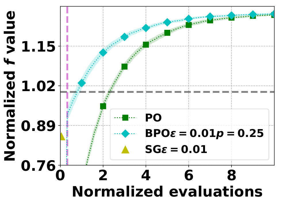 Figure 1
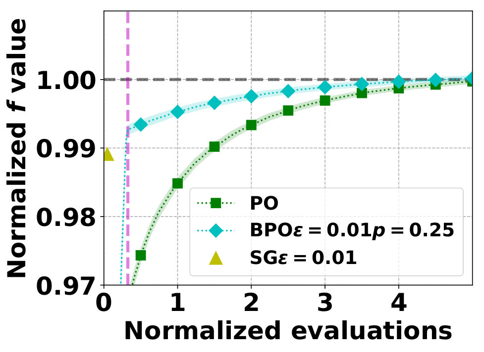 Figure 2
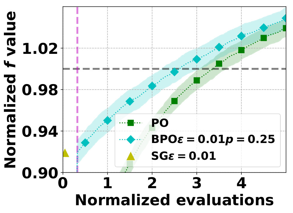 Figure 3
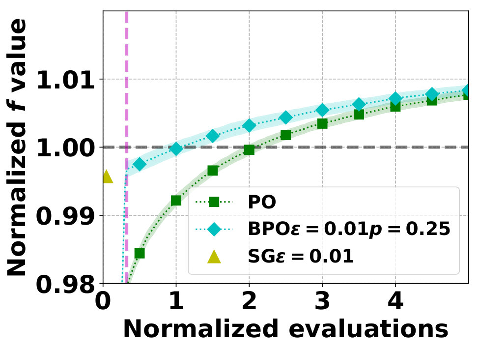 Figure 4
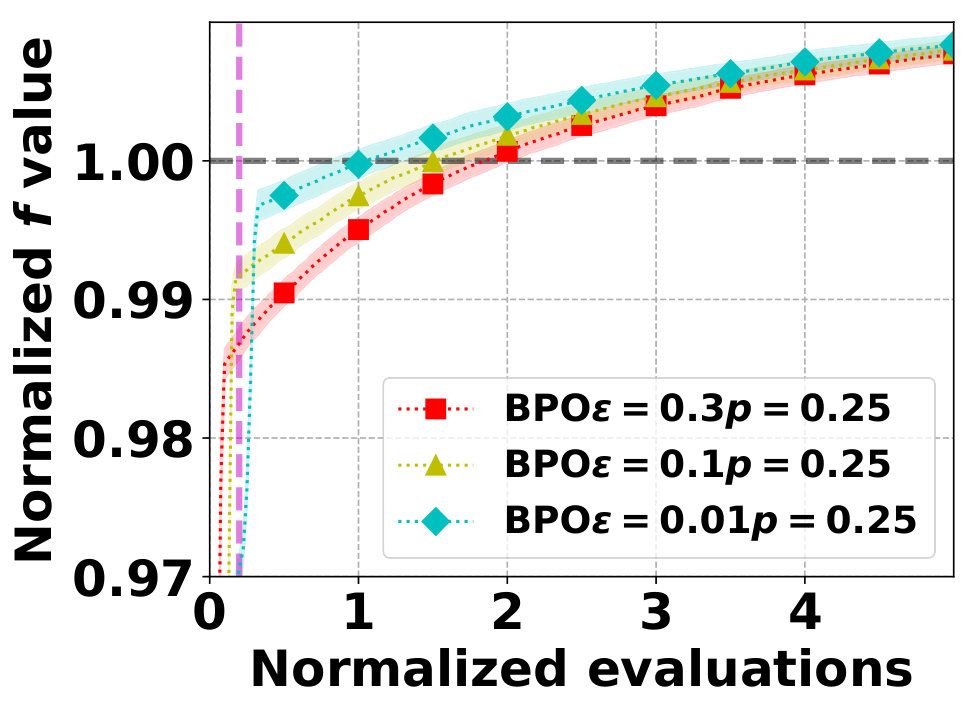 Figure 5
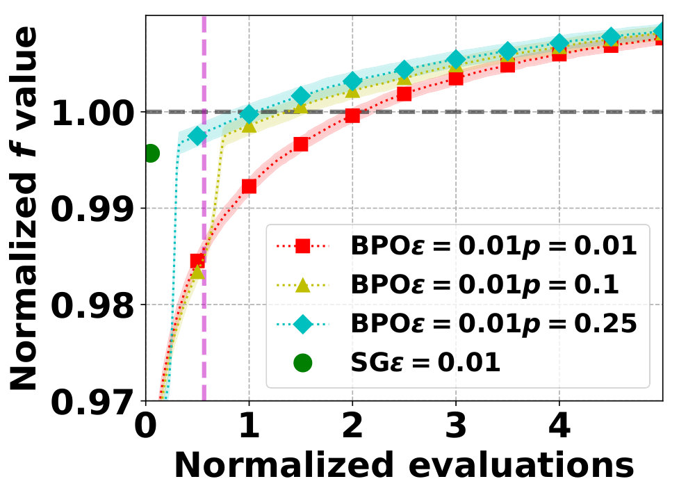 Figure 6
Peer Reviews
No public reviews on file for this paper yet. If you reviewed it on a platform where reviews are public (OpenReview, ICLR, NeurIPS, ICML), you can paste yours below so the community can read it here.
Videos
No videos yet. Explain this paper in a talk, walkthrough, or lecture? Add one.
Faster Guarantees of Evolutionary Algorithms for Maximization of Monotone Submodular Functions
Victoria G. Crawford University of Florida [email protected]
Abstract
In this paper, the monotone submodular maximization problem (SM) is studied. SM is to find a subset of size from a universe of size that maximizes a monotone submodular objective function . We show using a novel analysis that the Pareto optimization algorithm achieves a worst-case ratio of in expectation for every cardinality constraint , where is an input, in queries of . In addition, a novel evolutionary algorithm called the biased Pareto optimization algorithm, is proposed that achieves a worst-case ratio of in expectation for every cardinality constraint in queries of . Further, the biased Pareto optimization algorithm can be modified in order to achieve a worst-case ratio of in expectation for cardinality constraint in queries of . An empirical evaluation corroborates our theoretical analysis of the algorithms, as the algorithms exceed the stochastic greedy solution value at roughly when one would expect based upon our analysis.
1 Introduction
A function defined on subsets of a ground set of size is monotone submodular if it possesses the following two properties: (i) For all , (monotonicity); (ii) For all and , (submodularity). Monotone submodular set functions are found in many applications in machine learning and data mining. Applications of SM include influence in social networks Kempe et al. (2003), data summarization Mirzasoleiman et al. (2013), dictionary selection Das and Kempe (2011), and monitor placement Soma and Yoshida (2016). As a result, there has been much recent interest in optimization problems involving monotone submodular functions. One such optimization problem is the NP-hard Submodular Maximization Problem (SM), defined as follows.
Problem 1** (Submodular Maximization Problem (SM)).**
Let be a monotone submodular function defined on subsets of the ground set of size , and . Given a budget , SM is to find
An instance of SM is referred to as SM. It is assumed that the function is provided as a value oracle, which when queried with a set returns the value of . Time is measured in queries of , as is the convention in submodular optimization Badanidiyuru et al. (2014).
To approximate SM, the standard greedy algorithm is very effective. Nemhauser and Wolsey Nemhauser and Wolsey (1978) showed that the standard greedy algorithm achieves the best ratio of for SM in queries to . In addition, faster versions of the greedy algorithm have been developed for SM Badanidiyuru et al. (2014); Mirzasoleiman et al. (2015). In particular, the stochastic greedy algorithm (SG) of Mirzasoleiman et al. Mirzasoleiman et al. (2015) achieves ratio in expectation in queries to .
Alternatively, one may take the Pareto optimization approach to SM: Instead of maximizing for a cardinality constraint , SM is re-formulated as a bi-objective optimization problem where the goal is to both maximize as well as minimize cardinality. Instead of a single solution, we seek a pool of solutions none of which dominate another111In this context, a solution dominates if , , and at least one of the two inequalities is strict.. Greedy algorithms can be used to develop such a pool, however previous works Friedrich and Neumann (2014); Qian et al. (2015b) have employed bi-objective evolutionary algorithms because they iteratively improve the entire pool of solutions and can be run indefinitely. The evolutionary algorithm Pareto Optimization (PO) has previously been shown to find a approximate solution to SM for all , where is an input, in expected queries to Friedrich and Neumann (2014). Further, PO has been demonstrated to make significant empirical improvements over the standard greedy algorithms for SM Qian et al. (2015b). But as the size of data has grown exponentially in recent times, a query complexity that is cubic in (for ) makes these evolutionary algorithms a less attractive option.
1.1 Contributions
In this work, a novel analysis is provided for the algorithm PO, and it is proven that PO achieves a worst-case ratio of in expectation for every instance SM with , where is an input, in queries of . This removes a factor of from the query complexity of Friedrich and Neumann Friedrich and Neumann (2014). This novel analysis has potential to improve the query complexity of other problems in monotone submodular optimization beyond SM Qian et al. (2015a, 2017); Crawford (2019); Bian et al. (2020). This result is proven in Theorem 1.
Next, a novel algorithm Biased Pareto Optimization (BPO) is proposed that is a similar in spirit but faster version of PO for SM. It is proven that BPO achieves a worst-case ratio of in expectation for every instance SM with in queries of . This result is proven in Theorem 2. Further, a version of BPO for a specific cardinality constraint , -Biased Pareto Optimization (-BPO), is proven to achieve a worst-case ratio of in expectation for instance SM in queries of . This result is proven in Theorem 3. This new algorithm -BPO thus matches the optimal SG algorithm in terms of both approximation ratio and query complexity, while maintaining the ability of PO to continuously improve a pool of solutions.
The above theoretical results all extend to the more general setting of monotone -weakly submodular222 A function is -weakly submodular if for all , and , . If , then is submodular. functions Das and Kempe (2011), but with different approximation guarantees that depend on .
An empirical evaluation corroborates our theoretical analysis of the algorithms, as the algorithms exceed the SG solution value at roughly when one would expect based upon our analysis.
1.2 Additional Related Work
Evolutionary algorithms have been studied for many combinatorial optimization problems Laumanns et al. (2002); Neumann and Wegener (2007); Friedrich et al. (2010). In particular, evolutionary algorithms have been analyzed for problems in submodular optimization including SM Friedrich and Neumann (2014); Qian et al. (2015b); Roostapour et al. (2019), submodular cover Qian et al. (2015a); Crawford (2019), SM with more general cost constraints Bian et al. (2020), and noisy versions of SM Qian et al. (2017).
Friedrich and Neumann Friedrich and Neumann (2014) studied a slight variant of PO where the pool is initialized to contain a random set, and . Friedrich and Neumann proved that their variant of PO finds a approximate solution to SM in expected queries of . It is easy to modify their analysis to see that PO finds a approximate solution to SM for all in expected queries of . The argument of PO used in the proof of Theorem 1 of Section 2.1 is substantially different compared to the argument of Friedrich and Neumann because it analyzes the expected time until an expected approximation ratio is analyzed, resulting in a speedup to queries of . In addition, the result of Theorem 1 is in deterministic time due to an application of the Chernoff bound.
Qian et al. Qian et al. (2015b) considered the subset selection problem, which is a special case of the monotone -weakly submodular maximization problem. Qian et al. fixed , and showed that for the cardinality constraint PO finds a approximate solution in expected queries of . Their results can be generalized beyond subset selection to the monotone -weakly submodular maximization problem with cardinality constraint .
The algorithm BPO, presented in Section 2.2, uses a novel, biased selection procedure to identify sets for mutation. Because of the biased selection procedure, BPO is the first evolutionary algorithm that has an approximation guarantee in nearly linear queries of close to that of the greedy algorithm for SM.
2 Algorithms and Theoretical Results
The theoretical contributions of the paper are presented in this section. In particular, a new theoretical analysis of the algorithm Pareto Optimization (PO) is presented for SM in Section 2.1, the novel algorithm Biased Pareto Optimization (BPO) is presented and analyzed for SM in Section 2.2, and the faster modification of BPO for a specific cardinality constraint, -Biased Pareto Optimization (-BPO), is presented and analyzed for SM in Section 2.3. The full version of the paper includes an appendix where additional theoretical details from Section 2 are filled in.
Definitions and Notation
The following notation and definitions will be used throughout Section 2. Let , , and . (i) Marginal gain: . (ii) The membership of is flipped in means that if , then is removed from ; and if , then is added to . (iii) If is a random variable, then denotes the expected value of . If is a random event, then denotes the probability of occurring. (iv) Let . Then if there exists a unique such that , define . If no such exists, or there are multiple elements of of cardinality , is undefined. (v) Let . Then if and . If at least one of the two inequalities is strict, then and dominates . If and then it is said that is equivalent to .
2.1 Pareto Optimization (PO)
In this section, it is proven that in time , PO produces a approximate solution in expectation for every cardinality constraint , where is an input. If for a fixed cardinality constraint , then PO produces solutions for SM with similar theoretical guarantees to that of the standard greedy algorithm in the same asymptotic time, which shows the practicality of evolutionary algorithms such as PO for SM.
2.1.1 Description of PO
In this section, PO (Alg. 1) is described. The set is referred to as the pool, and each iteration of the for loop is referred to as an iteration. The pool initially contains only the empty set; its maximum size is determined by input parameter . During each iteration, is chosen uniformly randomly (Line 5 of Alg. 1), and if exists then it is selected from to be mutated, otherwise PO continues to the next iteration. The subroutine Mutate takes and randomly mutates it into as follows: for each , flip the membership of in with probability . Finally, if no set in the pool dominates or is equivalent to and , then is added to the pool and all sets that dominates are removed. There is at most one new query of on each iteration of PO, and therefore the input is equal to the query complexity. Pseudocode for the subroutine Mutate is provided in the appendix.
2.1.2 Analysis of PO for SM
In this section, the approximation result of the algorithm PO for SM is presented. Omitted proofs are given in the appendix. The statement of Theorem 1 easily generalizes to -weakly submodular objectives , where is replaced with .
Theorem 1**.**
Suppose PO is run with input , where is monotone submodular, , and . Let be the pool of PO at the end of iteration . Then for any ,
[TABLE]
Overview of Proof of Theorem 1
Given SM with optimal solution , the standard greedy algorithm iteratively picks into its solution the element in of highest marginal gain until elements have been picked. Existing analyses of PO for SM Friedrich and Neumann (2014); Qian et al. (2015b) analyze the time it takes until essentially the standard greedy algorithm randomly occurs within PO. If instead of iteratively picking the element of highest marginal gain, a uniformly random element of (possibly already chosen) is picked into the solution until elements are picked (this could be viewed as an idealized version of the stochastic greedy algorithm of Mirzasoleiman et al. Mirzasoleiman et al. (2015)) then the same approximation guarantee as the standard greedy algorithm () is achieved in expectation. In the proof of Theorem 1, the expected time until this second algorithm randomly occurs within PO is analyzed, which is a factor of faster.
Proof.
Line numbers referenced are those in Algorithm 1. Throughout the proof of Theorem 1, the probability space of all possible runs of PO with the stated inputs is considered. Let , and let . We may assume that , since is monotone. In the proof of Theorem 1, the random variable will be used, defined inductively as follows:
- (i)
Before the first iteration of PO, is set to [math].
- (ii)
If the following two conditions are met, is incremented at the end of an iteration:
- is selected on Line 5; and 2) Mutate on Line 8 results in the membership of a single element being flipped (i.e., it is either the case that Mutate returns for or for ).
Intuitively, is used to track a solution within that has a high value relative to its cardinality. In particular, the following lemma describes the key property of .
Lemma 1**.**
At the end of every iteration of PO
[TABLE]
where .
A further key point is that once a solution appears in PO, i.e., it is returned by Mutate, there always exists at least as good of a solution within .
Lemma 2**.**
Let and . If is returned by Mutate during iteration of PO, then at the end of any iteration it holds that
Let event be that at the completion of a run of PO, . Then it follows from Lemmas 1 and 2 that
[TABLE]
Then the remainder of the proof of Theorem 1 is to deal with the probability that reaches . To this end, the following lemma states that the run of PO may be interpreted as a Bernoulli process.
Lemma 3**.**
Consider a run of PO as a series of Bernoulli trials , where each iteration is a trial and a success is defined to be when is incremented. Then are independent, identically distributed Bernoulli trials where the probability of success is
[TABLE]
Then Lemma 3 and the Chernoff bound can be used to prove that the probability of not reaching after iterations of PO is small. This is stated in the following lemma.
Lemma 4**.**
**
Finally, Theorem 1 follows from the law of total expectation, Inequality 1 and Lemma 4. ∎
2.2 Biased Pareto Optimization (BPO)
Biased Pareto Optimization (BPO) is a novel evolutionary algorithm with nearly the same approximation results as PO for SM in faster time. Specifically, it is proven that in time , BPO finds a -approximate solution in expectation for every cardinality constraint , where is an input. Thus, BPO is faster than PO by a factor of ; further, it works similarly to PO but has a biased selection procedure instead of choosing uniformly randomly.
2.2.1 Description of BPO
In this section, BPO (Alg. 2) is presented. Pseudocode for BPO can be found in Alg. 2. In overview, BPO follows a similar iterative procedure to PO: every iteration of the for loop, a set in the is chosen for mutation; and only sets that are not dominated by any others are kept. The difference from PO is in the selection of the set for mutation; a certain subset of sets in are selected more frequently than others, as determined by the parameters , , and , and the variables for , where . There is at most one new query of on each iteration of BPO, and therefore the input is equal to the query complexity. Next, the selection process is described in detail.
Selection process
During each iteration, with probability BPO chooses from uniformly randomly (Line 9) and then sets (Line 10). Otherwise is chosen uniformly randomly from (Line 7). If exists then it is selected from to be mutated, otherwise BPO continues to the next iteration. Initially, . is incremented to if on H_{j}=$$e\ln(1/\epsilon)/\xi^{j} iterations since the last increment of was chosen on Line 9. The variable is used to determine when should be incremented: is incremented during an iteration if and only if is set to 0 on Line 13. Notice that if , BPO is equivalent to PO.
2.2.2 Analysis of BPO for SM
The approximation results of BPO for SM are now presented. Lemmas referenced in the proof of Theorem 2 can be found in the appendix. The statement of Theorem 2 easily generalizes to -weakly submodular objectives , where is replaced with .
Theorem 2**.**
Suppose BPO is run with input where is monotone submodular, , , where and , , , and . Let be the pool of BPO at the end of iteration . Then for any ,
[TABLE]
Overview of Proof of Theorem 2
Consider SM with optimal solution . Recall that in the proof of Theorem 1 in Section 2.1, the approximation ratio for SM was proven by analyzing the expected time until a variable reaches . In order for to be incremented during an iteration, must be selected on Line 5, which occurs with probability . If we instead consider an alternative version of PO where the selection is biased towards choosing with constant probability , then reaches faster. The difficulty is that the value of is unknown, since it depends on Mutate flipping the membership of an and nothing else. The idea behind BPO is that we can approximately track , and therefore bias the selection. In particular, for each SM with , there exists a that is approximately equal to the corresponding for .
Proof.
Proofs of lemmas used can be found in the appendix. Lines numbers referenced are those in Algorithm 2. Throughout the proof of Theorem 2, the probability space of all possible runs of BPO with the stated inputs is considered. An iteration of the for loop in BPO is simply referred to as an iteration.
Consider any . Define . Without loss of generality we may assume that , since is monotone. There exists such that
[TABLE]
Then define .
The defined here serves a similar purpose to that defined in the proof of Theorem 1; To track a solution within that has a high value relative to its cardinality, as described in the following lemma.
Lemma 5**.**
At the end of every iteration of BPO
[TABLE]
where .
In addition, the property of PO detailed in Lemma 2 of Theorem 1 clearly also holds for BPO.
Define the event to be that at the completion of a run of BPO has been incremented (Line 11 of Algorithm 2) times. If has been incremented times, then one may see that has been incremented times. Once reaches , it clearly follows from Lemmas 5 and 2 that
[TABLE]
where .
We now analyze the probability that has been incremented times. To this end, we have the following lemma.
Lemma 6**.**
Consider a run of BPO as a series of Bernoulli trials , where each iteration is a trial and a success is defined to be when is incremented. Then are independent, identically distributed Bernoulli trials where the probability of success is .
Finally, an analogous argument to that of Theorem 1 can be used to complete the proof of Theorem 2. In particular, we bound the probability of event not occurring after , where and , iterations of BPO by using the Chernoff bound, and then apply the law of total expectation. The details of the argument can be found in the appendix. ∎
2.3 -Biased Pareto Optimization (-BPO)
If a specific cardinality constraint is provided, a modified version of BPO, -Biased Pareto Optimization (-BPO), can produce an approximate solution in expectation even faster than BPO. In this section, the algorithm -BPO is described, and it is proven that -BPO finds a -approximate solution to SM in queries of .
2.3.1 Description of -BPO
Pseudocode for -BPO can be found in the appendix. -BPO is similar to BPO except -BPO is only biased towards picking a single element of , determined by the variable . The input parameters of -BPO are the same as BPO except is not needed.
During each iteration, with probability -BPO sets . Otherwise is chosen uniformly randomly from . If exists then it is selected from to be mutated, otherwise -BPO continues to the next iteration. Initially, . is incremented to if on iterations since the last increment of , was chosen to be . The variable is used to determine when should be incremented: is incremented during an iteration if and only if is set to 0.
2.3.2 Analysis of -BPO for SM
The approximation results of -BPO for SM are now presented. The statement of Theorem 3 easily generalizes to -weakly submodular objectives in the analogous manner as BPO.
Theorem 3**.**
Suppose -BPO is run with input where is monotone submodular, , , , and . Let be the pool of -BPO at the end of iteration . Then,
[TABLE]
Proof.
The proof of Theorem 3 is any easy modification of the proof of Theorem 2 and therefore details are left to the reader. The key point is that Lemma 6 should be replaced with the following lemma.
Lemma 7**.**
Consider a run of -BPO as a series of Bernoulli trials , where each iteration is a trial and a success is defined to be when is incremented. Then are independent, identically distributed Bernoulli trials where the probability of success is .
∎
3 Experimental Evaluation
In this section, the algorithms PO and -BPO are evaluated on instances of data summarization with submodular and non-submodular objectives . In summary, the faster runtime for PO proven in Theorem 1 is demonstrated empirically. Also, the results demonstrate that -BPO quickly finds solutions better than the standard greedy algorithm, the stochastic greedy algorithm SG Mirzasoleiman et al. (2015), and PO.
The algorithms evaluated in Section 3 are:
- •
the standard greedy algorithm Nemhauser and Wolsey (1978)
- •
the stochastic greedy (SG) algorithm of Mirzasoleiman et al. (2015).
- •
PO: the variant of the algorithm of Friedrich and Neumann Friedrich and Neumann (2014) as detailed in Alg. 1 and analyzed in Section 2.1.
- •
-BPO: the version of BPO that biases towards only one set in , based on the input as discussed in Section 2.3.
For both PO and -BPO, the parameter is used on all instances.
3.1 Application
In data summarization (DS), we have a set of data points and we wish to find a subset of of cardinality that best summarizes the entire dataset . takes to a measure of how effectively summarizes . For the ground set , we use: (i) A set of 10 dimensional vectors drawn from gaussian distributions (Gaussian), and (ii) a set of color images from the CIFAR-100 dataset Krizhevsky et al. (2009) each represented by a 3072 dimensional vector of pixels (CIFAR). For the objective , we use: (i) The monotonic and submodular objective -medoid objective Kaufman and Rousseeuw (2009) (), and (ii) the monotone weakly submodular objective based on Determinantal Point Process (DPP) Kulesza et al. (2012) (). A lower bound on the submodularity ratio has been proven for the latter objective Bian et al. (2017).
3.2 Results
The experimental results are shown in Figure 1. All results are the mean of repetitions of each algorithm; shaded regions represent one standard deviation from the mean. Objective and runtime are normalized by the objective value of and number of queries made () by the standard greedy algorithm. The value of the solution of the standard greedy algorithm is plotted as a dotted gray horizontal line . The time where in -BPO reached is plotted as a vertical magenta line.
The best solution value obtained by each algorithm is shown as the rightmost point in each plot. Both -BPO and PO were eventually able to find better solutions than the standard greedy algorithm (i.e., normalized value ), especially on the non-submodular objective (Figures 1(e) and 1(f)). Observe that PO typically exceeds the stochastic greedy objective value within , where . This behavior corroborates our theoretical analysis that PO achieves a good solution in expectation in queries. In addition, -BPO exceeds the SG value in queries. Finally, for PO, recall that the theoretical anlaysis shows that for any , the approximation ratio holds.
Because PO and -BPO can be terminated at any time, the running time may be compared by observing where any vertical line intersects the curves for each algorithm. The running time of the standard greedy corresponds to the line (not plotted). -BPO reaches solution values closer to the standard greedy algorithm in significantly faster time than PO, as expected by its design. The effect of varying the parameters and on the behavior of -BPO is shown in Figs. 1(c), 1(d), respectively: smaller leads to a higher initial increase but the initial increase is slower, while smaller slows down the rate of the initial increase.
4 Conclusions
In this work, we have re-analyzed the evolutionary algorithm PO, originally analyzed for submodular maximization by Friedrich and Neumann Friedrich and Neumann (2014), and showed that it achieves nearly the optimal worst-case ratio in expectation on SM for any in queries. In contrast, Friedrich and Neumann Friedrich and Neumann (2014) showed that the optimal worst-case ratio is achieved in expected queries. This improved rate of convergence is supported by an empirical evaluation.
Further, it has been shown that changing the selection process in PO results in improved query complexity to to obtain the same approximation results. A variant of this algorithm -BPO is shown empirically to have a much faster initial rate of convergence to a good solution than PO, without sacrificing the long-term behavior of the PO algorithm.
5 Appendix: Algorithms and Theoretical Results
In this section, additional results from Section 2 are included. In particular: Pseudocode missing from the description of the algorithm PO is given in Section 5.1.1; Lemmas used in Section 2.1 and their corresponding proofs are given in Section 5.1.2; Lemmas used in Section 2.2 and their corresponding proofs are given in Section 5.2.1; Finally, pseudocode for -BPO is given in Section 5.3
5.1 Pareto Optimization (PO)
5.1.1 Additional Pseudocode
5.1.2 Lemmas used for the Proof of Theorem 1
Lemma 1.
At the end of every iteration of PO
[TABLE]
where .
Proof.
At the end of any iteration of PO, define (i) to be the value of , and (ii) . Define and refer to the values at the start of the first iteration. In order to prove Lemma 1, it must be shown that at the end of any iteration ,
[TABLE]
Equation 4 will be proven by induction on iteration . Equation 4 is clearly true for , since on all runs of BPO and . Now suppose that Equation 4 is true for iteration ; it will be shown that it is then true for iteration .
Define to be the event that during iteration of the for loop of PO, is incremented by 1. The following claim establishes that expected value of does not depend on .
Claim 1**.**
**
Proof.
At the beginning of iteration the probability that will be incremented is
[TABLE]
This does not depend on the value of , so for all , . Then Bayes’ theorem gives that , which implies Claim 1. ∎
Inequality 4 is proven by breaking up into the two cases and , and then applying the law of total probability. If did not occur, then it follows from Lemma 2 that
[TABLE]
where the last inequality follows from the inductive assumption and the fact that when conditioning on .
The proof will proceed by considering arbitrary but fixed runs of PO. Consider runs of PO where did occur. If occurs, then during iteration , is selected on Line 5 and then Mutate results in the membership of a single being flipped in , i.e. it is either the case that Mutate returns for or for .
Claim 2**.**
The following holds:
Proof.
If occurs, then Mutate returns either for or for . Let be the former event and let be the latter event.
Consider a particular run of PO where occurs. Then . If occurs on this run, then was returned by Mutate on iteration and therefore by Lemma 2. If occurs on this run, then . was returned by Mutate on some run before since at the end of iteration . Therefore by Lemma 2. Then for any run of PO where occurs and so Claim 2 follows. ∎
Next, it holds that
[TABLE]
where (a) follows from Claim 2; (b) follows from Lemma 8; (c) is by Claim 1; (d) is the inductive assumption; (e) is because by definition of , . Finally, the inductive step follows by Equations 5, 6 and the law of total probability. Therefore Lemma 1 is proven. ∎
Lemma 2
*Let and . If is returned by Mutate during iteration of PO, then at the end of any iteration it holds that
Proof.
First, notice that once has been returned by Mutate, there exists such that from that point in PO on. Consider the end of any iteration . Let be such that at the end of iteration . Then since . ∎
Lemma 3.
Consider a run of PO as a series of Bernoulli trials , where each iteration is a trial and a success is defined to be when is incremented. are independent, identically distributed Bernoulli trials where the probability of success is
[TABLE]
Proof.
In order for to be incremented on an iteration (i.e. the trial results in a success), the set must be selected on Line 5; this occurs with probability . In addition, if any set is selected, Mutate results in flipping of the membership of a single and nothing else, with probability Therefore, the probability of success is . This probability is independent of the iteration , and therefore it follows that are independent and identically distributed. ∎
Lemma 4.
Consider a run of PO as a series of Bernoulli trials , where each iteration is a trial and a success is defined to be when is incremented. Then
[TABLE]
Proof.
By Lemma 3, Chernoff’s bound (Lemma 9) may be applied to . Let be the probability of success for each (the value of is given in Lemma 3). Then . Therefore
[TABLE]
where (a) is because combined with the lower bound on given in Lemma 3; (b) is applying Lemma 9 with ; and (c) is because combined with the lower bound on given in Lemma 3. ∎
Lemma 8**.**
Let , . Suppose that is input to Mutate, and consider the probability space of all possible outputs of Mutate. Let be the event that Mutate returns for some or for some . Then
[TABLE]
Proof.
It is clear from the procedure Mutate that the event is equivalent to uniformly randomly choosing and then flipping its membership in . Then it is the case that
[TABLE]
where (a) follows from the monotonicity and submodularity of . ∎
Lemma 9** (Chernoff bound).**
Suppose are independent random variables taking values in . Let denote their sum and let denote the sum’s expected value. Then for any
[TABLE]
5.2 Biased Pareto Optimization (BPO)
5.2.1 Lemmas used for the Proof of Theorem 2
Lemma 5
At the end of every iteration of BPO
[TABLE]
*where .
Proof.
For notational simplicity we define , and . and are defined analogously as in the proof of Lemma 1: At the end of any iteration of BPO, define (i) to be the value of , and (ii) . and refer to the values at the start of the first iteration. We see in Claim 3 that the objective values of the sequence are non-decreasing.
Claim 3**.**
For any run of BPO, if then .
Proof.
only increases throughout BPO, therefore . Then if is the pool at the end of iteration
[TABLE]
where (a) follows from Lemma 2. ∎
In order to prove Lemma 5 it must be shown that for any iteration ,
[TABLE]
which will be proven using induction on . Equation 7 is clearly true for , since on all runs of BPO and . Now suppose that Equation 7 is true for every iteration ; It will now be shown that Equation 7 is true for iteration .
Define the random variable . In other words is the iteration during which was incremented to equal , which is the value of at the beginning of iteration . Then is not incremented on any iteration in . We will be using the inductive assumption on iteration in order to prove Equation 7. Define the events and as follows:
- (i)
Event is that during iteration of BPO, is incremented. Observe that if occurred, then during iteration of BPO was incremented to equal . Since is set to 0 during iteration , this implies that that on distinct iterations of BPO was incremented. In other words, on each of these iterations the set is chosen for mutation. Event is illustrated in Figure 2.
- (ii)
Event is defined to be that occurred and further that during one of the iterations Mutate resulted in the membership of a single element being flipped and it was an element of , i.e. it is either the case that Mutate returns for or for . Event is illustrated in Figure 3.
We now prove a couple of results concerning the events and . Claim 4 states that if occurs then does as well with high probability. Claim 5 states that the expected value of is independent of event .
Claim 4**.**
.
Proof.
At the beginning of any iteration the probability that Mutate will result in the flipping of a single element in and no other changes is
[TABLE]
Therefore the probability that has been selected on Line 18 times and on none of those iterations did Mutate result only in the flipping of a single element in is
[TABLE]
where (a) follows from Equation 2. Claim 4 then follows. ∎
Claim 5**.**
**
Proof.
Let . First it is shown that . On any iteration of BPO, the probability that will be incremented is . Whether it increments times in the interval does not depend on the value of , therefore .
Next, it is shown that . If it is assumed that occurred and so is incremented times in the interval , then on each of these increments the probability that Mutate results only in the flipping of a single element in is
[TABLE]
This does not depend on the value of , therefore .
Then we use the above two facts to see that . Then Bayes’ theorem gives that , which implies the statement of Claim 5. ∎
Equation 7 will be proven by breaking up runs of BPO into those where occurs and doesn’t occur, then further breaking up runs of BPO where occurs into those where occurs and doesn’t occur, and finally applying the law of total probability. The case of runs of BPO where does not occur is an easy result of Lemma 2:
[TABLE]
We now consider runs of BPO where event occurs. If occurred, then on some iteration Mutate resulted in the membership of an being flipped and no other changes. Now two needed claims are proven. Claim 6 states that if occurs then the expected value of is at least the expected value of , while Claim 7 gives a lower bound on the expected value of . Together, these two claims provide a lower bound on the expected value of if occurs.
Claim 6**.**
**
Proof.
If occurs, then Mutate returns either for or for . Let be the former event and let be the latter event.
Consider a particular run of BPO where occurs. Then since did not increment on runs in but did on iteration . If occurs on this run, then was returned by Mutate on iteration and therefore by Lemma 2. If occurs on this run, then . was returned by Mutate on some run before since at the end of iteration . Therefore by Lemma 2. Then for any run of PO where occurs and so Claim 2 follows. ∎
Claim 7**.**
**
Proof.
Consider all runs of BPO where occurs. Then it can be seen by inspecting Mutate that any element of is equally likely to be the one flipped. Therefore
[TABLE]
where (a) follows from the monotonicity and submodularity of . Claim 7 follows by re-arranging the equation. ∎
Now we can apply the above claims in order to see that
[TABLE]
where (a) is applying Claims 6 and 7; (b) is applying Claim 3; and (c) is applying Claim 5. Finally
[TABLE]
where (a) is because by Claim 3 and by Claim 5; (b) is using Equation 9; (c) is using Claim 4; (d) is using the inductive assumption; and (e) is because if occurred then . Finally, the inductive step follows by Equations 8, 10 and the law of total probability. Therefore Lemma 5 is proven. ∎
Lemma 6
*Consider a run of BPO as a series of Bernoulli trials , where each iteration is a trial and a success is defined to be when is incremented. are independent, identically distributed Bernoulli trials where the probability of success is .
Proof.
In order for to be incremented, the element in of cardinality must be chosen by Select-BPO, which one can see by inspecting Select-BPO that this occurs with probability . ∎
End of Proof of Theorem 2
By Lemma 6, we are able to apply Chernoff’s bound (Lemma 9) to . By seeing that \mathbb{E}\left[\sum_{i=1}^{T}Y_{i}\right]=T$$p/\lceil\ln(P)/\ln\left(1/\xi\right)\rceil,
[TABLE]
where (a) is because ; (b) is applying Lemma 9 with ; and (c) is because .
5.3 -Biased Pareto Optimization (-BPO)
The reference list from the paper itself. Each links out to its DOI / PubMed record.
- 1Badanidiyuru et al. (2014) Ashwinkumar Badanidiyuru, Baharan Mirzasoleiman, Amin Karbasi, and Andreas Krause. Streaming submodular maximization: massive data summarization on the fly. In ACM SIGKDD International Conference on Knowledge Discovery and Data Mining (KDD) , 2014.
- 2Bian et al. (2017) Andrew An Bian, Joachim M Buhmann, Andreas Krause, and Sebastian Tschiatschek. Guarantees for greedy maximization of non-submodular functions with applications. In International Conference on Machine Learning (ICML) , 2017.
- 3Bian et al. (2020) Chao Bian, Chao Feng, Chao Qian, and Yang Yu. An efficient evolutionary algorithm for subset selection with general cost constraints. In AAAI Conference on Artificial Intelligence (AAAI) , 2020.
- 4Crawford (2019) Victoria G. Crawford. An efficient evolutionary algorithm for minimum cost submodular cover. In International Joint Conference on Artificial Intelligence (IJCAI) , 2019.
- 5Das and Kempe (2011) Abhimanyu Das and David Kempe. Submodular meets Spectral: Greedy Algorithms for Subset Selection, Sparse Approximation and Dictionary Selection. Proceedings of the 28th International Conference on Machine Learning (ICML) , 2011.
- 6Friedrich and Neumann (2014) Tobias Friedrich and Frank Neumann. Maximizing submodular functions under matroid constraints by evolutionary algorithms. In International Conference on Parallel Problem Solving from Nature (PPSN) , 2014.
- 7Friedrich et al. (2010) Tobias Friedrich, Jun He, Nils Hebbinghaus, Frank Neumann, and Carsten Witt. Approximating covering problems by randomized search heuristics using multi-objective models. Evolutionary Computation , 18(4):617–633, 2010.
- 8Kaufman and Rousseeuw (2009) Leonard Kaufman and Peter J Rousseeuw. Finding groups in data: an introduction to cluster analysis , volume 344. John Wiley & Sons, 2009.