Central-limit theorem for conservative fragmentation chains
Sylvain Rubenthaler (JAD)

TL;DR
This paper establishes a central-limit theorem for the empirical measure of fragments in a conservative fragmentation process, extending previous convergence results and providing insights into the distributional fluctuations of small fragments.
Contribution
It introduces a central-limit theorem for the empirical measure of fragments in a conservative fragmentation chain, under specific assumptions, advancing the understanding of their probabilistic behavior.
Findings
Proves a central-limit theorem for the empirical measure of fragments
Provides bounds on the rate of convergence in fragmentation processes
Enhances understanding of fluctuations in fragment sizes
Abstract
We are interested in a fragmentation process. We observe fragments frozen when their sizes are less than ( > 0). Is is known ([BM05]) that the empirical measure of these fragments converges in law, under some renormalization. In [HK11], the authors show a bound for the rate of convergence. Here, we show a central-limit theorem, under some assumptions.
Click any figure to enlarge with its caption.
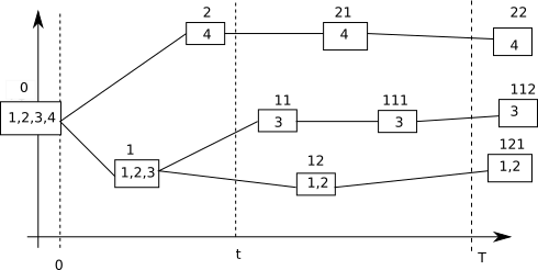 Figure 1
Peer Reviews
No public reviews on file for this paper yet. If you reviewed it on a platform where reviews are public (OpenReview, ICLR, NeurIPS, ICML), you can paste yours below so the community can read it here.
Videos
No videos yet. Explain this paper in a talk, walkthrough, or lecture? Add one.
Taxonomy
TopicsStochastic processes and statistical mechanics · Theoretical and Computational Physics · Markov Chains and Monte Carlo Methods
Central-limit Theorem for conservative fragmentation chains
Sylvain Rubenthaler
(Date: March 17, 2024)
Abstract.
We are interested in a fragmentation process. We observe fragments frozen when their sizes are less than (). Is is known ([BM05]) that the empirical measure of these fragments converges in law, under some renormalization. In [HK11], the authors show a bound for the rate of convergence. Here, we show a central-limit theorem, under some assumptions.
1. Introduction
1.1. Scientific and economic context
One of the main goals in the mining industry is to extract blocks of metallic ore and then separate the metal from the valueless material. To do so, rock is fragmented into smaller and smaller rocks. This is carried out in a series of steps, the first one being blasting, after which the material goes through a sequence of crushers. At each step, the particles are screened, and if they are smaller than the diameter of the mesh of a classifying grid, they go to the next crusher. The process stops when the material has a sufficiently small size (more precisely, small enough to enable physicochemical processing).
This fragmentation process is energetically costly (each crusher consumes a certain quantity of energy to crush the material it is fed). One of the problems that faces the mining industry is that of minimizing the energy used. The optimisation parameters are the number of crushers and the technical specifications of these crushers.
In [BM05], the authors propose a mathematical model of what happens in a crusher. In this model, the rock pieces/fragments are fragmented independently of each other, in a random and auto-similar manner. This is consistent with what is observed in the industry, and this is supported by the following publications: [PB02, DM98, Wei85, Tur86]. Each fragment has a size (in ) and is then fragmented into smaller fragments of sizes , , … such that the sequence has a law which does not depend on (which is why the fragmentation is said to be auto-similar). This law is called the dislocation measure (each crusher has its own dislocation measure). The dynamic of the fragmentation process is thus modelized in a stochastic way.
In each crusher, the rock pieces are fragmented repetitively until they are small enough to slide through a mesh whose holes have a fixed diameter. So the fragmentation process stops for each fragment when its size is smaller than the diameter of the mesh, which we denote by (). We are interested in the *statistical distribution *of the fragments coming out of a crusher. If we renormalize the sizes of these fragments by dividing them by , we obtain a measure , which we call the *empirical measure *(the reason for the index instead of will be made clear later). In [BM05], the authors show that the energy consumed by the crusher to reduce the rock pieces to fragments whose diameters are smaller than can be computed as an integral of a bounded function against the measure (they cite [Bon52, Cha57, WLMG67] on this particular subject). For each crusher, the empirical measure is one of the two only observable variables (the other one being the size of the pieces pushed into the grinder). The specifications of a crusher are summarized in and .
1.2. State of the art
In [BM05], the authors show that the energy consumed by a crusher to reduce rock pieces of a fixed size into fragments whose diameter are smaller than behaves asymptotically like a power of when goes to zero. More precisely, this energy multiplied by a power of converges towards a constant of the form (the integral of , the dislocation measure, against a bounded function ). In [BM05], the authors also show a law of large numbers for the empirical measure . More precisely, if is bounded continuous, converges in law, when goes to zero, towards an integral of against a measure related to (this result also appears in [HK11], p. 399). We set to be this limit (check Equations (5.1), (2.5), (2.2) to get an exact formula). The empirical measure thus contains information relative to and one could extract from it an estimation of or of an integral of any function against .
It is worth noting that by studying what happens in various crushers, we could study a family (with an index for the number of the crusher and the index for the -th test function in a well-chosen basis). Using statistical learning methods, one could from there make a prediction for ) for a new crusher for which we know only the mechanical specifications (shape, power, frequencies of the rotating parts …). It would evidently be interesting to know before even building the crusher.
In [HKK10], the authors prove a convergence result for the empirical measure similar to the one in [BM05], the convergence in law being replaced by an almost sure convergence. In [HK11], the authors give a bound on the rate of this convergence, in a sense, under the assumption that the fragmentation is conservative. This assumption means there is no loss of mass due to the formation of dust during the fragmentation process.
So we have convergence results ([BM05, HKK10]) of an empirical quantity towards constants of interest (a different constant for each test function ). Using some transformations, these constants could be used to estimate the constant . Thus it is natural to ask what is the exact rate of convergence in this estimation, if only to be able to build confidence intervals. In [HK11], we only have a bound on the rate.
When a sequence of empirical measures converges to some measure, it is natural to study the fluctuations, which often turn out to be Gaussian. For such results in the case of empirical measures related to the mollified Boltzmann equation, one can cite [Mel98, Uch88, DZ91]. When interested in the limit of a -tuple as in Equation (1.1) below, we say we are looking at the convergence of a -statistics. Textbooks deal with the case where the points defining the empirical measure are independent or with a known correlation (see [dlPG99, DM83, Lee90]). The problem is more complex when the points defining the empirical measure are in interaction with each other like it is the case here.
1.3. Goal of the paper
As explained above, we want to obtain the rate of convergence in the convergence of when goes to zero. We want to produce a central-limit theorem of the kind: for a bounded continuous , converges towards a non-trivial measure when goes to zero (the limiting measure will in fact be Gaussian), for some exponent . The technics used will allow us to prove the convergence towards a multivariate Gaussian of a vector of the kind
[TABLE]
for functions , …, .
More precisely, if by , , …, we denote the fragments sizes that go out from a crusher (with mesh diameter equal to ). We would like to show that for a bounded continuous ,
[TABLE]
and that for all , and , …, bounded continuous function such that ,
[TABLE]
converges in law towards a multivariate Gaussian when goes to zero.
The exact results are stated in Proposition 5.1 and Theorem 5.2.
1.4. Outline of the paper
We will state our assumptions along the way (Assumptions A, B, C, D). Assumption D can be found at the beginning of Section 3. We define our model in Section 2. The main idea is that we want to follow tags during the fragmentation process. Let us imagine the fragmentation is the process of breaking a stick (modeled by ) into smaller sticks. We suppose that the original stick has painted dots and that during the fragmentation process, we take note of the sizes of the sticks supporting the painted dots (we call them the painted sticks). When the sizes of the painted sticks get smaller than (), the fragmentation is stopped for these sticks. In Section 3, we make use of classical results on renewal processes and of [Sgi02] to show that the size of one painted stick has an asymptotic behavior when goes to zero and that we have a bound on the rate with which it reaches this behavior. Section 4 is the most technical. There we study the asymptotics of symmetric functionals of the sizes of the painted sticks (always when goes to zero). In Section 5, we precisely define the measure we are interested in ( with ). Using the results of Section 4, it is then easy to show a law of large numbers for (Proposition 5.1) and a central-limit Theorem (Theorem 5.2). Proposition 5.1 and Theorem 5.2 are our two main results. The proof of Theorem 5.2 is based on a simple computation involving characteristic functions (the same technique was already used in [DPR09, DPR11a, DPR11b, Rub16]).
1.5. Notations
For in , we set , . The symbol means “disjoint union”. For in , we set . For an application from a set to a set , we write if is injective and, for in , if , we set
[TABLE]
2. Statistical model
2.1. Fragmentation chains
Let . Like in [HK11], we start with the space
[TABLE]
A fragmentation chain is a process in characterized by
- •
a dislocation measure which is a finite measure on ,
- •
a description of the law of the times between fragmentations.
A fragmentation chain with dislocation measure is a Markov process with values in . Its evolution can be described as follows: a fragment with size lives for some time (which may or may not be random) then splits and gives rise to a family of smaller fragments distributed as , where is distributed according to . We suppose the life-time of a fragment of size is an exponential time of parameter , for some . We could here make different assumptions on the life-time of fragments, but this would not change our results.
We denote by the law of started from the initial configuration with in . The law of is entirely determined by and (Theorem 3 of [Ber02]).
We make the same assumption as in [HK11] and we will call it Assumption A.
Assumption A**.**
We have and .
Let
[TABLE]
denote the infinite genealogical tree. For and , we say that is in the -th generation and we write , and we write , for all . For any and (), we say that is the ancestor of . For any in ( deprived of its root), has exactly one ancestor and we denote it by . The set is ordered alphanumerically :
- •
If and are in and then .
- •
If and are in and and , with , … , , then .
A mark is an application from to some other set. We associate a mark on the tree to each path of the process . The mark at node is , where is the size of the fragment indexed by . The distribution of this random mark can be described recursively as follows.
Proposition 2.1**.**
*(Consequence of Proposition 1.3, p. 25, [Ber06]) There exists a family of i.i.d. variables indexed by the nodes of the genealogical tree, , where each is distributed according to the law , and such that the following holds:
Given the marks of the first generations, the marks at generation are given by*
[TABLE]
where and is the child of .
2.2. Tagged fragments
From now on, we suppose that we start with a block of size . We assume that the total mass of the fragments remains constant through time, as follows.
Assumption B**.**
(Conservative property).
We have .
2.2.1. First definition
We can now define tagged fragments. We use the representation of fragmentation chains as random infinite marked tree to define a fragmentation chain with tagged fragments. Suppose we have a fragmentation process . On each node , we set a mark
[TABLE]
with defined as above and , denoting the tags present on the fragment labeled by . The random variables are defined as follows.
- •
We set .
- •
We suppose we have i.i.d. random variables of law . For all , given the marks of the first generations, the marks at generation are given by Proposition 2.1 (concerning ) and
[TABLE]
We observe that, for all , , ,
[TABLE]
In the case , the branch has the same law as the randomly tagged branch of Section 1.2.3 of [Ber06]. The presentation is simpler in our case because the Malthusian exponent is under Assumption B.
2.2.2. Second definition
There is a different way to define the law of the random mark , which we will present now. This definition is strictly equivalent to the first definition above. We take to be i.i.d. variables of law . We set, for all in ,
[TABLE]
with defined as above. The random variables take values in the subsets of . The random variables take values in . These variables are defined as follows.
- •
We set , .
- •
For all , given the marks of the first generations, the marks at generation are given by Proposition 2.1 (concerning ) and
[TABLE]
[TABLE]
We obtain having the same law as in Section 2.2.1. So the two definitions are equivalent.
2.3. Observation scheme
We ofreeze the process when the fragments become smaller than a given threshold . That is, we have the following data
[TABLE]
where
[TABLE]
We now look at tagged fragments (). For each in , we call , , … the successive sizes of the fragment having the tag . More precisely, for each , there is almost surely exactly one such that , ; and so, . For each , the process is a renewal process without delay, with waiting-time following a law (see [Asm03], Chapter V for an introduction to renewal processes). This law is defined by the following.
[TABLE]
(see Proposition 1.6, p. 34 of [Ber06], or Equations (3), (4), p. 398 of [HK11]).
We make the following assumption on .
Assumption C**.**
There exist () such that the support of is . We set .
We set
[TABLE]
We set, for all , , ****
[TABLE]
The process is a homogeneous Markov process (Proposition 1.5 p. 141 of [Asm03]). We call it the residual lifetime of the fragment tagged by . In the following, we will treat as a time parameter. This has nothing to do with the time in which the fragmentation process evolves.
We observe that, for all , is exchangeable (meaning that for all in the symmetric group of order , has the same law as ).
2.4. Stationary age process
We define to be an independent copy of . We suppose it has tagged fragments. Therefore it has a mark and renewal processes (for all in ) defined in the same way as for . We let be the residual lifetimes of the fragments tagged by and .
Let
[TABLE]
and let be the distribution with density with respect to . We set to be a random variable of law . We set to be independent of and uniform on . We set . The process , , , , … is a renewal process with delay . We set to be its residual lifetime process :
[TABLE]
Theorem 3.3 p.151 of [Asm03] tells us that has the same transition as defined above and that is stationary.
We define a measure on by its action on bounded measurable functions:
[TABLE]
Lemma 2.2**.**
The measure is the law of (for any ).
Proof.
Let . We set , for all in . We have (with of law )
[TABLE]
∎
For in , we now want to define a process having the same transition as and being stationary. We set such that it has the law . As we have given its transition, the process is well defined in law. In addition, we suppose that it is independent of all the other processes.
For in , we define a process such that and has the law of conditioned on
[TABLE]
which reads as follows : the tag remains on the fragment bearing the tag until the size of the fragment is smaller than . We observe that, conditionally on , : and are independent.
Let in be such that
[TABLE]
Now we state a small Lemma that will be useful below.
Lemma 2.3**.**
Let be in The variables and have the same support (and it is ).
Proof.
By Equation (2.4), the support of is ; and so the support of is . By Assumption C, the support of is and the support of is . If then . As and are independent, we get that the support of includes (because of Equation (2.6)). As this support is included in , we have proved the desired result. ∎
For in , we define a process by: has the law of
[TABLE]
conditioned on . This conditioning is correct because and have the same support.
3. Rate of convergence in the Key Renewal
Theorem
We need the following regularity assumption.
Assumption D**.**
The probability is absolutely continuous with respect to the Lebesgue measure (we will write ). The density function is continuous on .
Fact 3.1**.**
Let ( is fixed in the rest of the paper). The density satisfies
[TABLE]
For a nonnegative Borel-measurable function on , we set to be the set of complex-valued measures (on the Borelian sets) such that , where stands for the total variation norm. If is a finite complex-valued measure on the Borelian sets of , we define to be the -finite measure with the density
[TABLE]
Let be the cumulative distribution function of .
We set (see Equation (2.3) for the definition of , , …). By Theorem 3.3 p.151 and Theorem 4.3 p. 156 of [Asm03], we know that converges in law to a random variable (of law ). The following Theorem is a consequence of [Sgi02], Theorem 5.1, p. 2429. It shows there is actually a rate of convergence for this convergence in law.
Theorem 3.2**.**
Let . Let
[TABLE]
If is a random variable of law then
[TABLE]
as approaches outside a set of Lebesgue measure zero (the supremum is taken on in the set of Borel-measurable functions on ).
Proof.
Let stands for the convolution product. We define the renewal measure (notations: , the Dirac mass at [math], ( times)). We take i.i.d. variables of law . We set , for all in . We have, for all ,
[TABLE]
We set
[TABLE]
We have, for all ,
[TABLE]
We have: . The function is submultiplicative and it is such that
[TABLE]
The function is in . The function is in . We have as . We have
[TABLE]
We have .
Let us now take a function such that . We set
[TABLE]
Then we have and (computing as above for )
[TABLE]
So, by [Sgi02], Theorem 5.1, we have proved the desired result. ∎
Corollary 3.3**.**
There exists a constant bigger than such that: for any bounded measurable function on such that ,
[TABLE]
for outside a set of Lebesgue measure zero.
Proof.
We take in the above Theorem. Keep in mind that is defined in Equation (2.5). There exists a constant such that: for all measurable function such that ,
[TABLE]
Let us now take a bounded measurable such that . By Equation (3.1), we have (for outside a set of Lebesgue measure zero)
[TABLE]
∎
4. Limits of symmetric functionals
4.1. Notations
We fix . We set to be the symmetric group of order . A function is symmetric if
[TABLE]
For , we define a symmetric version of by
[TABLE]
We set to be the set of bounded, measurable, symmetric functions on , and we set to be the of such that
[TABLE]
We set
[TABLE]
Suppose that is in and . For in , we consider the following collections of nodes of :
[TABLE]
[TABLE]
We set to be the set of leaves in the tree . For in and in , there exists one and only one in such that . We call it . Under Assumption C, there exists a constant bounding the numbers vertices of almost surely. Let us look at an example in Figure 4.1.
Here, we have a graphic representation of a realization of . Each node of is written above a rectangular box in which we read ; the right side of the box has the coordinate on the -axis. For simplicity, the node is designated by , the node is designated by , and so on. In this example: , , , , …, , , , , .
For , in , we define the event
[TABLE]
For example, in Figure 4.1, we are in the event .
We define
[TABLE]
[TABLE]
For example, in Figure 4.1, . Let be in . We observe that is measurable with respect to if (we suppose that this is the case in the following). We set, for all in , . Let be the set of leaves in the tree such that the set has a single element . For example, in Figure 4.1, .
For even () and for all in , we define the events
[TABLE]
[TABLE]
We set, for all in ,
[TABLE]
4.2. Intermediate results
Lemma 4.1**.**
We suppose that is in and that is of the form . Let be in . For any in , in and in , we have
[TABLE]
(for a constant defined below in the proof) and
[TABLE]
[TABLE]
Proof.
We have . Let be in . Since the event is in , we have
[TABLE]
If in and if , then, conditionally on , , is independent of all the other variables and has the same law as . Thus, using Theorem 3.2 and Corollary 3.3, we get, for any , , ,
[TABLE]
Thus we get
[TABLE]
For a fixed , we have
[TABLE]
where, for all ,
[TABLE]
We observe that, for all :
[TABLE]
[TABLE]
and if is such that
[TABLE]
for some integers , , then for all ,
[TABLE]
We observe that, under Assumption C, there exists a constant which bounds almost surely and so there exists a constant which bounds almost surely. So, we have
[TABLE]
As , then , and so we have proved the desired result. ∎
Lemma 4.2**.**
Let be an integer . Let . We have
[TABLE]
where .
Let be an integer . Let . We have
[TABLE]
Proof.
Let be an integer and let . We decompose
[TABLE]
where
[TABLE]
Suppose we are in the event . For and for all in such that , we define
[TABLE]
[TABLE]
We have
[TABLE]
If we suppose that and , then
[TABLE]
∎
Immediate consequences of the two above lemmas are the following Corollaries.
Corollary 4.3**.**
If is odd and if is of the form , then
[TABLE]
[TABLE]
Proof.
We take . We can decompose
[TABLE]
∎
Corollary 4.4**.**
Suppose is of the form . Let in . Then
[TABLE]
Proof.
[TABLE]
∎
We now want to find the limit of when goes to [math], for even. First we need a technical lemma.
For any , the process has a stationary law (see Theorem 3.3 p. 151 of [Asm03]). Let be a random variable having this stationary law (it has already appeared in Section 3). We can always suppose that it is independent of all the other variables.
Lemma 4.5**.**
Let , be in . Let belong to . We have
[TABLE]
and
[TABLE]
where
[TABLE]
Proof.
From now on, we suppose that , (this is true if is large enough). We have, for all in ,
[TABLE]
And so,
[TABLE]
We have
[TABLE]
We have
[TABLE]
We observe that, for all in ,
[TABLE]
[TABLE]
for some function (the same on both lines) such that . So, by Theorem 3.2 and Corollary 3.3, the quantity in Equation (4.2) can be bounded by
[TABLE]
(coming from Corollary 3.3 there is an integral over a set of Lebesgue measure zero in the above bound, but this term vanishes). The above bound can in turn be bounded by:
[TABLE]
We have
[TABLE]
and
[TABLE]
Equations (4.1), (4.3), (4.4) and (4.5) give us the desired result. ∎
Lemma 4.6**.**
Let in . We suppose is even and . Let . We suppose , with , … , in . We then have :
[TABLE]
Proof.
We have
[TABLE]
By Lemma 4.5, we have, for some constant ,
[TABLE]
We introduce the events (for )
[TABLE]
and the tribes (for in , )
[TABLE]
We have :
[TABLE]
We then observe that
[TABLE]
and, for ,
[TABLE]
So
[TABLE]
This finishes the proof of Equation (4.6).
∎
4.3. Convergence result
For and bounded measurable functions, we set
[TABLE]
For even, we set to be the set of partitions of into subsets of cardinality . For in and in , we introduce
[TABLE]
For in , we define
[TABLE]
Proposition 4.7**.**
Let be in . Let with , …, in . If is even () then
[TABLE]
Proof.
Let be in . We have
[TABLE]
By Lemma 4.1 and Lemma 4.2, we have that
[TABLE]
(because is exchangeable). We compute :
[TABLE]
∎
5. Results
We are interested in the probability measure defined by its action on bounded measurable functions by
[TABLE]
We define, for all in , from to ,
[TABLE]
[TABLE]
where the last sum is taken over all the injective applications from to . If we set
[TABLE]
then
[TABLE]
[TABLE]
We define, for all bounded continuous ,
[TABLE]
Proposition 5.1** (Law of large numbers).**
Let f be a continuous function from to . We have:
[TABLE]
Proof.
We take a bounded measurable function . We define . We take an integer . We introduce the notation :
[TABLE]
We have
[TABLE]
We now take sequences , . We then have, for all and for all ,
[TABLE]
So, by Borell-Cantelli’s Lemma,
[TABLE]
Let be in . We can decompose
[TABLE]
For in , we set . We can then write
[TABLE]
So we have, for all ,
[TABLE]
If we take , the two terms in the equation above can be transformed:
[TABLE]
[TABLE]
Let . We fix in . Almost surely, there exists such that, for , . For , we can then write (still with ):
[TABLE]
Let and in . We can decompose
[TABLE]
For in , we set . For any continuous from to , there exists such that, for all , . Suppose that . Then we have (for all ),
[TABLE]
Equations (5.2) and (5.4) prove the desired result. ∎
Theorem 5.2** (Central-limit Theorem).**
Let be in . For functions , …, which are continuous and in , we have
[TABLE]
( is given in Equation (5.5)).
Proof.
Let , …, and .
First, we develop the product below
[TABLE]
where
[TABLE]
[TABLE]
We have, for some constant ,
[TABLE]
Second, we develop the same product in a different manner. We have
[TABLE]
By Corollary 4.4, we have, for all ,
[TABLE]
So, by Corollary 4.3 and Proposition 4.7, we get that
[TABLE]
In conclusion, we have
[TABLE]
So we get the desired result with, for all , ,
[TABLE]
( is defined in Equation (4.9)). ∎
The reference list from the paper itself. Each links out to its DOI / PubMed record.
- 1[Asm 03] Søren Asmussen, Applied probability and queues , second ed., Applications of Mathematics (New York), vol. 51, Springer-Verlag, New York, 2003, Stochastic Modelling and Applied Probability. MR 1978607
- 2[Ber 02] Jean Bertoin, Self-similar fragmentations , Ann. Inst. H. Poincaré Probab. Statist. 38 (2002), no. 3, 319–340. MR 1899456
- 3[Ber 06] by same author, Random fragmentation and coagulation processes , Cambridge Studies in Advanced Mathematics, vol. 102, Cambridge University Press, Cambridge, 2006. MR 2253162 (2007 k:60004)
- 4[BM 05] Jean Bertoin and Servet Martínez, Fragmentation energy , Adv. in Appl. Probab. 37 (2005), no. 2, 553–570. MR 2144567
- 5[Bon 52] F. C. Bond, The third theory of comminution , AIME Trans. 193 (1952), no. 484.
- 6[Cha 57] R. J. Charles, Energy-size reduction relationships in comminution , AIME Trans. 208 (1957), 80–88.
- 7[dl PG 99] Víctor H. de la Peña and Evarist Giné, Decoupling , Probability and its Applications (New York), Springer-Verlag, New York, 1999, From dependence to independence, Randomly stopped processes. U 𝑈 U -statistics and processes. Martingales and beyond. MR MR 1666908 (99k:60044)
- 8[DM 83] E. B. Dynkin and A. Mandelbaum, Symmetric statistics, Poisson point processes, and multiple Wiener integrals , Ann. Statist. 11 (1983), no. 3, 739–745. MR MR 707925 (85b:60015)