Gravitational redshift test with the future ACES mission
Etienne Savalle, Christine Guerlin, Pac\^ome Delva, Fr\'ed\'eric, Meynadier, Christophe le Poncin-Lafitte, Peter Wolf

TL;DR
This paper evaluates the ACES space mission's ability to test gravitational redshift, demonstrating that with realistic noise and data conditions, the mission can achieve its precision goals within a few measurement sessions.
Contribution
The authors develop simulation tools and analysis methods to assess ACES's gravitational redshift test performance under realistic conditions.
Findings
Target uncertainty of 2-3 ppm is achievable within a few measurement sessions.
Achieving the test precision requires orbit determination accuracy of about 300 meters.
Realistic noise and data gaps do not significantly hinder the test's success.
Abstract
We investigate the performance of the upcoming ACES (Atomic Clock Ensemble in Space) space mission in terms of its primary scientific objective, the test of the gravitational redshift. Whilst the ultimate performance of that test is determined by the systematic uncertainty of the on-board clock at 2-3 ppm, we determine whether, and under which conditions, that limit can be reached in the presence of colored realistic noise, data gaps and orbit determination uncertainties. To do so we have developed several methods and software tools to simulate and analyse ACES data. Using those we find that the target uncertainty of 2-3 ppm can be reached after only a few measurement sessions of 10-20 days each, with a relatively modest requirement on orbit determination of around 300 m.
Click any figure to enlarge with its caption.
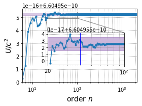 Figure 1
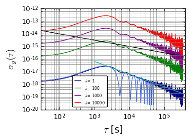 Figure 2
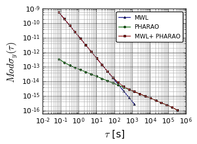 Figure 3
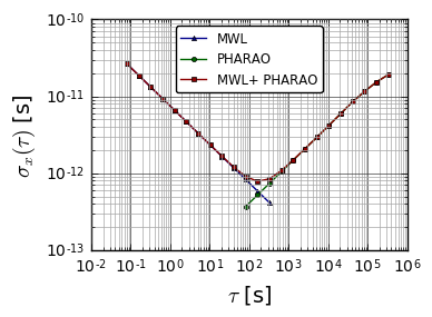 Figure 4
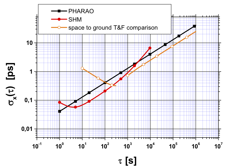 Figure 5
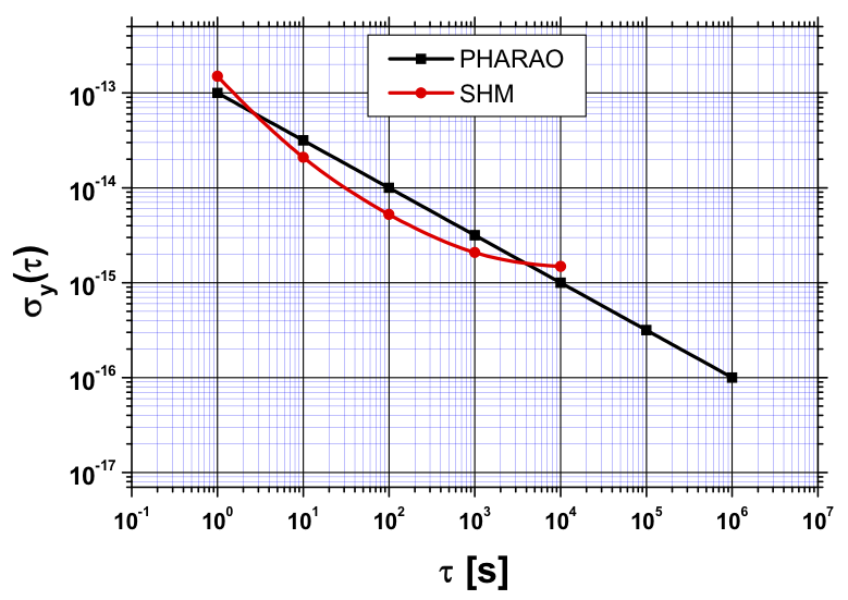 Figure 6
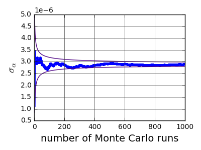 Figure 7
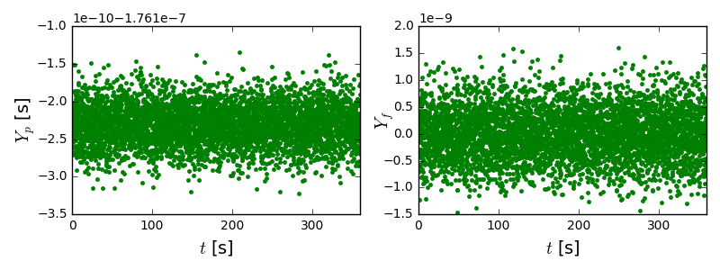 Figure 8
 Figure 9
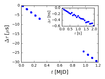 Figure 10
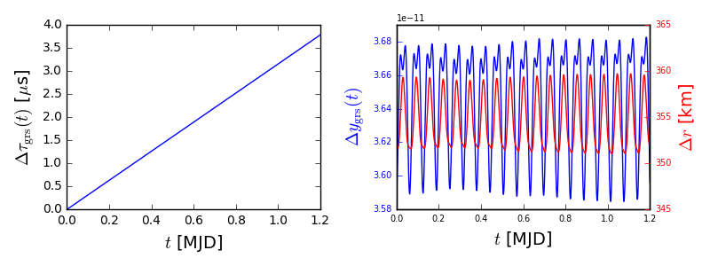 Figure 11
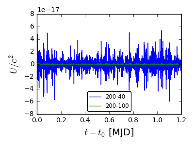 Figure 12
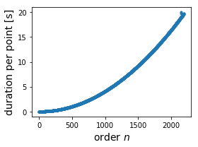 Figure 13
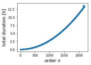 Figure 14
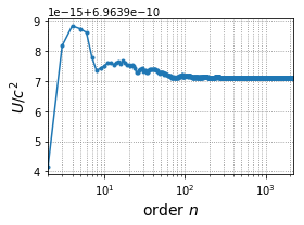 Figure 15
 Figure 16
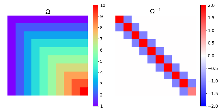 Figure 17
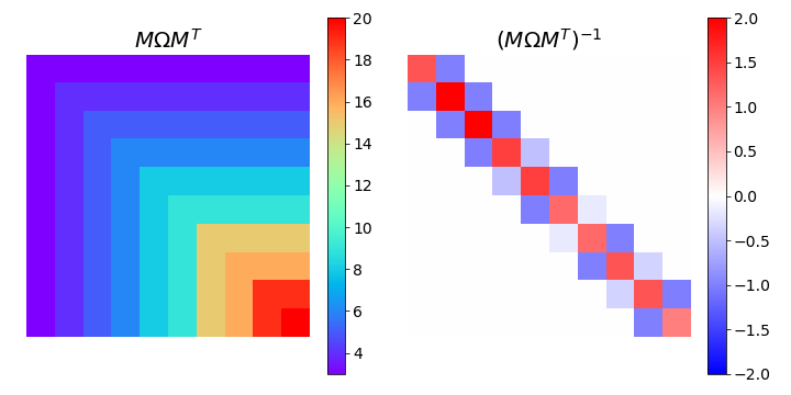 Figure 18
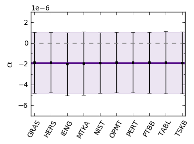 Figure 19
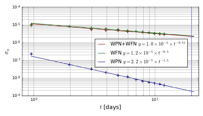 Figure 20
 Figure 21
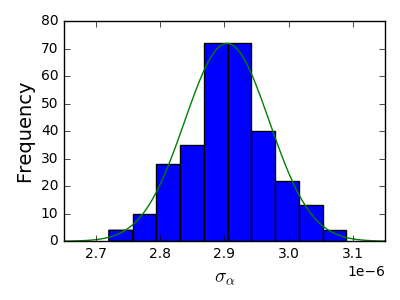 Figure 22
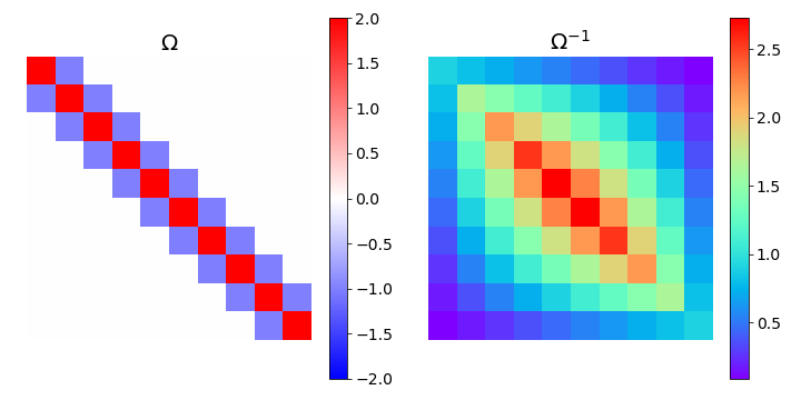 Figure 23
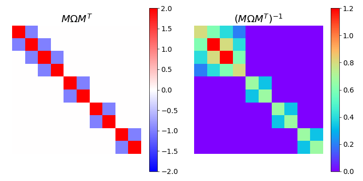 Figure 24
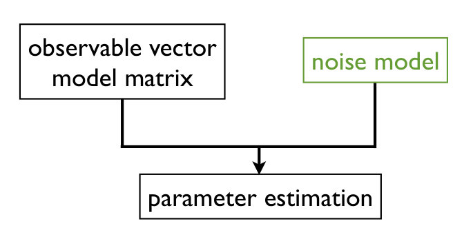 Figure 25
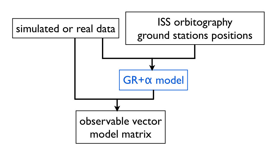 Figure 26
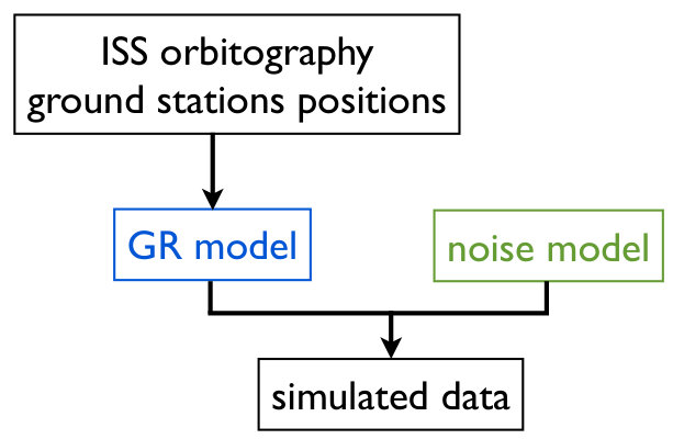 Figure 27
| Label | Laboratory | Location | Latitude (∘) | Longitude (∘) | Height (m) |
|---|---|---|---|---|---|
| OPMT | OBSPM | Paris, FR | 48.8 | 2.3 | 124.2 |
| PTBB | PTB | Braunschweig, DE | 52.3 | 10.5 | 130.2 |
| HERS | NPL | Hailsham, UK | 50.9 | 0.3 | 76.5 |
| NISU | NIST | Boulder, US | 40.0 | -105.3 | 1648.5 |
| TABL | JPL | Wrightwood, US | 34.4 | -117.7 | 2228.0 |
| MTKA | NICT | Mitaka, JP | 35.7 | 139.6 | 109.0 |
| IENG | INRIM | Torino, IT | 45.0 | 7.6 | 316.6 |
| GRAS | OCA | Caussols, FR | 43.8 | 6.9 | 1319.3 |
| TSKB | GSI | Tsukuba, JP | 36.1 | 140.1 | 67.3 |
| PERT | UWA | Perth, AU | -31.8 | 115.9 | 12.9 |
| LSMC (1d) | GLS (1d) | LSMC (12d) | AGLS (12d) | |
|---|---|---|---|---|
| (s) | ||||
| Cor | -0.05 | -0.03 | -0.19 |
| Data distribution | Parameter | Frequency data | Phase data |
|---|---|---|---|
| realistic | |||
| (s) | |||
| Cor | -0.24 | ||
| continuous | |||
| (s) | |||
| Cor | -0.28 | ||
| first and last pass | |||
| (s) | |||
| Cor | -0.01 |
Peer Reviews
No public reviews on file for this paper yet. If you reviewed it on a platform where reviews are public (OpenReview, ICLR, NeurIPS, ICML), you can paste yours below so the community can read it here.
Videos
No videos yet. Explain this paper in a talk, walkthrough, or lecture? Add one.
- 25th June, 2019
Gravitational redshift test with the future ACES mission
E Savalle1,22footnotemark: 2, C Guerlin1,2,22footnotemark: 2, P Delva1, F Meynadier1,3, C le Poncin-Lafitte1, P Wolf1 00footnotetext: E. Savalle and C. Guerlin should be considered as co-first authors.
1SYRTE, Observatoire de Paris, Université PSL, CNRS, Sorbonne Université, LNE, 61 avenue de l’Observatoire, 75014 Paris, France
2Laboratoire Kastler Brossel, ENS-Université PSL, CNRS, Sorbonne Université, Collège de France, 24 rue Lhomond, 75005 Paris, France
3Bureau International des Poids et Mesures, Pavillon de Breteuil, 92312 Sèvres Cedex, France
Abstract
We investigate the performance of the upcoming ACES (Atomic Clock Ensemble in Space) space mission in terms of its primary scientific objective, the test of the gravitational redshift. Whilst the ultimate performance of that test is determined by the systematic uncertainty of the on-board clock at 2-3 ppm, we determine whether, and under which conditions, that limit can be reached in the presence of coloured realistic noise, data gaps and orbit determination uncertainties. To do so we have developed several methods and software tools to simulate and analyse ACES data. Using those we find that the target uncertainty of 2-3 ppm can be reached after only a few measurement sessions of 10-20 days each, with a relatively modest requirement on orbit determination of 300 m.
1 Introduction
General relativity (GR) together with all other metric theories of gravitation provides a geometrical description of the gravitational interaction. Fundamentally, such a description is based on the Einstein equivalence principle (EEP), itself the result of universal coupling of all standard matter to gravity. Although very successful so far, there are reasons to think that sufficiently sensitive measurements could uncover a failure of the EEP. For example, the unification of gravitation with the other fundamental interactions, and quantum theories of gravitation, generally lead to small deviations from the EEP (see e.g. [1]). Also dark matter and energy are so far only observed through their gravitational effects, but might be hints towards a modification of GR.
From a phenomenological point of view, three aspects of the EEP can be tested: (i) the universality of free fall (UFF); (ii) local Lorentz invariance (LLI); and (iii) local position invariance (LPI). Although the three are related, the quantitative details of that relation are model dependent [1, 2], so each of the three sub-principles needs to be tested independently to best possible uncertainty. UFF has been recently constrained by the Microscope space mission [3], while LLI was recently constrained, for example, by using a ground fibre network of optical clocks [4] (see e.g. [1, 5] for reviews). In this paper we focus on testing LPI.
LPI stipulates that the outcome of any local non-gravitational experiment is independent of the space-time position of the freely-falling reference frame in which it is performed. This principle is mainly tested by two types of experiments: (i) search for variations in the constants of Nature (see e.g. [6] for a review) and (ii) gravitational redshift tests. The gravitational redshift was observed for the first time in the Pound-Rebka-Snider experiment [7, 8, 9, 10].
One of the most accurate tests of the gravitational redshift has been realized with the Vessot-Levine rocket experiment in 1976, also named the Gravity Probe A (GP-A) experiment [11, 12, 13]. The frequency difference between a space-borne hydrogen maser clock and ground hydrogen masers was measured thanks to a continuous two-way microwave link. The total duration of the experiment was limited to 2 hours and reached an uncertainty of [13]. Very recently this has been surpassed by the analysis of clocks on board two eccentric Galileo satellites, reaching an uncertainty of [14, 15, 16].
In this work we study the expected performance of the gravitational redshift test using the ACES (Atomic Clock Ensemble in Space) mission, scheduled for launch in 2020. The heart of that mission is an accurate cold atom Cesium clock (PHARAO). It will be installed on an outside pallet of the Columbus module of the international space station (ISS) at 400 km altitude. Comparing that clock to ground clocks using a two-way microwave link (MWL) will allow performing a redshift test at an expected uncertainty of , limited by the systematic uncertainty of PHARAO. Here we investigate whether, and under which conditions, that goal can be reached when taking into account the main statistical noise contributions and the uncertainty from orbit determination errors.
The MWL and its data analysis has been described in [17], which also provides an estimate of the effect of orbit determination errors on the time transfer model, but not on the determination of the frequency shift of the clock. The latter has been studied to some extent in [18]. Here we study, in a full end to end scenario, the contribution of all noise sources (MWL, clocks), as well as the orbit determination errors, on the final scientific goal, i.e. the test of the gravitational redshift. To do so we use two software tools developed specifically for the ACES mission that simulate and analyse the data. The latter will be used for ACES data analysis when the mission will fly.
Our paper is organized as follows: Section 2 provides a brief description of the ACES space mission, its payload, and its specifications, together with a description of the gravitational redshift in that context. We conclude that section by an overview of our simulation and analysis software. Data simulation and analysis are then presented in details respectively in Sections 3 and 4. We describe different data observables and corresponding models, with an emphasis on parameters estimation in the presence of realistic noise and data gaps. We then provide our results concerning the gravitational redshift test accuracy (Section 5) and the required uncertainty on orbit determination (Section 6). Finally we conclude with a summary of our main results and a view towards the future in Section 7.
2 The ACES mission and the gravitational redshift
2.1 Overview
During 18 months up to 3 years, the ACES module will be attached to the ISS and up to 8 ground terminals (GT) will operate in ground laboratories [17, 19, 20, 21]. A two-way microwave link (MWL) will allow time comparison between ground clocks and the onboard timescale provided by the cold atom clock PHARAO and a hydrogen maser (SHM). Ground to space comparisons will be made when the ISS is in view of a given GT. The phase accumulated by the clocks between passes of the ISS is kept track of and allows the monitoring of the desynchronisation coherently over the typical duration of continuous operation of PHARAO and grounds clocks, which will be limited by the ISS environment (manoeuvring and other disturbances) to periods of typically 10-20 days. The primary scientific objective of the mission is to measure Einstein’s gravitational redshift at 2-3 ppm, improving the present best test [15, 16] by about a factor 10.
2.2 Einstein’s gravitational redshift
According to GR, the proper time of a clock near the Earth evolves as:
[TABLE]
where is the speed of light in vacuum, are the space-time coordinates in a geocentric non-rotating coordinate system (the Geocentric Coordinate Reference System, GCRS [22]), is the clock coordinate velocity in GCRS at coordinate time , and is the Newtonian potential at time and position (taken with the convention ). This expression is valid in the post-newtonian approximation, for low potential () and velocity (). Higher order terms in (1) have been investigated e.g. in [23, 24] and are negligible at the sensitivity of ACES. Other higher order terms of order can play a role in frequency transfer [25] at uncertainty in fractional frequency, but are negligible for the time transfer used in ACES.
In Eq. (1) the first term is the gravitational redshift, the second term is the second order Doppler effect from Special Relativity. The expression (1) is also equal to the frequency ratio between two clocks:
[TABLE]
where (resp. ) is the frequency of a clock at rest and at zero gravitational potential (resp. at non-zero gravitational potential and velocity). We define the fractional frequency shift between these two clocks as:
[TABLE]
where . Clocks at non-zero gravitational potential tick slower and are thus “red-shifted” by the gravitational potential.
The gravitational redshift can be measured by comparing two clocks ( and ) at different gravitational potentials, i.e. by determining . For a clock on ground in Paris (), the gravitational redshift is . For a space clock () on board the ISS (height above Paris 350 km), the gravitational redshift is . Thus PHARAO, considering only this term, ticks faster with a differential gravitational redshift of:
[TABLE]
The overall rate of PHARAO is actually slower than a static ground clock due to the bigger contribution of the Doppler effect term, for which the difference has opposite sign and is:
[TABLE]
Comparing the two clocks can be realized by exchanging electromagnetic signals, either by frequency comparison, or time comparison if one is able to monitor their desynchronization . Eq. (4) gives the contribution of the gravitational redshift term to the differential relative frequency shift. Their overall desynchronization can be obtained by integrating Eq. (1) :
[TABLE]
where is the initial phase offset between the two clocks. For a constant potential difference as given in Eq. (4), the gravitational redshift thus leads to a linear drift of the desynchronization by about 3 s per day.
A deviation from the gravitational redshift of General Relativity is commonly sought as a constant and isotropic deviation, where Einstein’s gravitational redshift is rescaled by a factor , with for GR [1, 2]. Assuming the measurement is limited only by the systematic effects on PHARAO frequency at , the sensitivity of the gravitational redshift test would reach an uncertainty on of about 2-3 ppm, improving by one order of magnitude the stringent test achieved using the accidental eccentricity of two Galileo satellites [14, 15, 16].
The aim of this work is to investigate whether, and under which conditions, this limit due to PHARAO systematic effects can be reached in terms of statistical uncertainty, when considering realistic noise levels for the space clock and clock comparison system.
2.3 ACES payload
ACES will realize an ultra-stable time scale using two atomic clocks: a hydrogen maser (SHM) and a cold atom Cesium clock (PHARAO). It contains also a GNSS (Global Navigation Satellite System) receiver for orbit determination and a Microwave Link (MWL) module for two way time and frequency transfer to ground terminals. Analysing raw data from this MWL retrieves the scientific products, among which the desynchronization between ground clocks and and the on-board time scale [18, 17].
Onboard ACES, the Frequency Comparison and Distribution Package (FCDP) allows the comparison of the SHM and PHARAO clock signal. It realizes a short-term servo loop that phase locks PHARAO’s local oscillator on SHM’s clock signal, and a long-term servo loop that frequency stabilizes the SHM local oscillator on PHARAO’s clock signal. FCDP combines both servo loops in order to generate the ACES clock signal, which inherits the short term stability of SHM and the long term stability and accuracy of PHARAO. For averaging times exceeding 10 days, the stability will be limited by the PHARAO systematic uncertainty of . FCDP provides this ACES clock signal to the MWL for comparison to ground clock signals.
2.4 ACES data
In the ACES mission, a given ground clock in a laboratory equipped with a MWL ground terminal will be compared to PHARAO when ISS is in sight. The time transfer software for extracting the clock desynchronization from MWL raw data has been presented in [17].
The altitude of ISS is kept between 330 and 435 km, with an inclination of with respect to the Earth equatorial plane, and an orbital period of about 90 minutes. For a given ground station, the passes last in average about 300 seconds (up to 500 seconds), with each day a series of typically 5-6 passes approximately every 90 minutes interrupted by longer out of view periods. The ground-PHARAO clock desynchronizations are measured every 80 ms of the local GT time scale, which will be considered here to be UTC. We call these “phase data”, from which relative frequency differences (“frequency data”) are derived. Simulated phase and frequency data, for 9 successive passes of PHARAO above a ground station located in Paris (OPMT), are shown on Figure 1. As can be seen, data have large gaps covering about 97% of the total duration.
Currently six fixed and two mobile MWL ground terminals are planned. The fixed ones will be located in National Metrology Institutes, equipped with high performance atomic clocks (e.g. Cesium/Rubidium fountains or optical clocks) with stabilities that outperform the ACES time scale, leaving the on-board clock and the MWL as the dominating noise contributors. For the tests presented here we considered 10 possible locations listed in Table 1. The MWL can operate on up to four channels, such that up to 4 ground stations can be compared to ACES simultaneously.
Auxiliary data (e.g. temperature, pressure, power levels, etc…) that allows correcting for numerous systematic effects will be available. The ones that are important in the context of this work are the ISS orbit and attitude data obtained from GNSS (Global Navigation Satellite System) receivers on the ISS and the ACES payload itself. Using that data the orbit of the PHARAO space clock reference point (the centre of its microwave cavity) can be retrieved.
2.5 Specifications
The frequency stability specifications of the two ACES clocks are shown on Figure 2 [20]. For short term variations (below a few s), SHM is more stable than PHARAO, whereas PHARAO is the more stable clock for long averaging times. PHARAO stability is characterized by white frequency noise with a stability goal of where is the averaging time in seconds. The target accuracy is and is reached after 10 days averaging.
The time stability specifications are shown on Figure 2 [20]. Over one pass ( 300 s) the MWL noise is white phase noise and its time deviation should average down to ps at 300 s. For longer averaging times the dominant noise comes from PHARAO.
2.6 Overview of the simulation and analysis software
We have developed a software that simulates ACES desynchronization data as will be obtained from raw MWL data using the methods described in [17]. It uses as basic input ISS orbitography files, ground station positions, a geopotential model, and PHARAO and MWL noise models. The software also allows calculating the model that needs to be adjusted to the data in order to search for a putative violation of the gravitational redshift, and carries out such an adjustment providing an estimate of the redshift violation parameter and its uncertainty.
It is written in Python3 and has approximately 3000 lines of code. It can be run in three modes:
simulation: simulates realistic data;
analysis: reads experimental or simulated data, and constructs the vector of observables and the model matrix that needs to be adjusted to it;
adjustment: adjusts the model matrix to the vector of observables and evaluates parameter values and uncertainties.
It is modular and makes use of common Python classes. As pictured on Fig. 3, the simulation and analysis modes have in common the construction of the GR model, and the simulation and adjustment modes have in common the generation of noise. Note that to estimate the effect of an orbitography error (Sec. 6), the analysis mode can be provided with an orbitography file that is different from the one used in the simulation mode, thus emulating imperfect knowledge of the orbit.
3 Data simulation
The MWL data processing presented in [17] will provide for each clock a file with coordinate time tags (in UTC) and corresponding ground clock/PHARAO desynchronization, every 80 ms during each pass, with a new file for each day.
However since no such real data are available yet, we simulate desynchronization data as will be provided by ACES MWL data analysis [17], as well as corresponding frequency data (discrete time derivative of the desynchronization data). For this we use the GR model of Equation (6), expressed in GCRS. This requires the knowledge of PHARAO and ground station orbitography in GCRS and the choice of a geopotential model (Subsection 3.2). The latter is given in a reference system rotating with the Earth, like the International Terrestrial Reference Frame (ITRF), see Subsection 3.3. We generate realistic time distribution of the data regarding repetition rate and pass distribution (Subsection 3.1). We also simulate different types of noise that affect the data (Subsection 3.4).
The input information for the simulation is the following:
fixed ground station position coordinates in ITRF2014 [26];
a real ISS orbitography file in SP3 format [27], with the spatial coordinates given in ITRF, and GPS time;
the Earth Geopotential Model 2008 (EGM2008) [28];
Earth Orientation Parameters (EOP) provided by IERS [29] for frame transformations;
instrumental noise levels.
For the simulation we used a 12-day ISS orbitography file provided by O. Montenbruck.
3.1 Simulation and realistic data distribution
We first simulate for each clock independently (ground clocks and PHARAO) the fractional frequency shifts from gravitational redshift and second order Doppler effect, whose sum, from Eqs. (1) and (3), is:
[TABLE]
We then calculate for each ground clock the PHARAO-ground clock difference for each term, and integrate them in order to have their contributions to desynchronization. This is done at every time of the orbitography file (time step 30 s for the files we used). Data are then cut in “passes” in order to keep them, for a given ground station, only when ISS is in line of sight, with a minimum elevation angle of . Each column (gravitational redshift differences and second order doppler shift differences, in phase and frequency) is then interpolated in order to have data every 80 ms. The sum of the two terms then gives the the overall differential frequency shift and desynchronization.
The noise on the PHARAO-ground clock difference is simulated every 80 ms and then cut with the same procedure. We simulate a single noise file for PHARAO, added to individual noise files for each ground station representing the MWL noise on their channel.
The main outputs of the simulation are time series of noisy fractional frequency differences and desynchronizations , for each ground clock-PHARAO couple, dated in UTC at 80 ms sampling.
For this simulation (and for the analysis), we use directly the orbitography file of the center of mass of ISS. For real data we will need to calculate the orbitography of the PHARAO clock, which requires the knowledge of the ISS attitude.
The model part of this software (without noise) has been tested against an independent software by Anja Schlicht and Stefan Marz at the Technical University of Munich (TUM). We checked that, in frequency, the potential and Doppler terms agree. This was done up to order 50 in potential for the ISS and 5 for the OPMT ground station. The space-ground gravitational redshift agrees within and the Doppler shift agrees within .
3.2 Geopotential
For the geopotential we use the model “Earth Geopotential Model 2008” (EGM 2008) [28], which gives the spherical harmonic coefficients of the static Earth potential at a given position in the reference system World Geodetic System 84 (WGS84) [30]. The difference between recent ITRF realizations and WGS84 being within 10 cm, we use directly the ITRF positions of ground clocks and PHARAO in order to calculate the geopotential at their position.
The gravitational redshift for the OPMT ground station and for the ISS, depending on the truncation order of the development, is shown respectively on Figures 4 and 4. The OPMT station is considered to have a fixed position with respect to ITRF, thus its potential has to be calculated only once for the simulation and analysis. Therefore we calculate the OPMT potential at the maximum order 2190. Whereas for ISS it has to be calculated at every point of the orbitography file (which with a spacing of 30 s over 12 days amounts to points) which takes several hours when using all orders.
To reduce the computational burden we checked whether the calculation can be safely truncated at a lower order without biasing the redshift analysis. The inset of Fig. 4 shows that above order 40, the redshift stays well within from the convergence value. Above 200, at this scale the variations of the redshift are not visible any more. Thus a safe choice for a realistic simulation can be to simulate and analyse at order 200. We checked on Fig. 4 that for all points of the orbitography used, the difference between the redshift at order 40 and 200 stays within a few parts in , and the comparison between order 100 and 200 confirms that for the desired precision the potential has indeed converged. As a final check, we run the full software, simulating with order 200 and analyzing with order 10 or higher: we obtain the same (non-significant) value and uncertainty irrespective of the order used.
As a consequence all tests presented below have been realized with order 200 for the ISS both for simulation and analysis. This is both self-consistent, and would retrieve safe values when analysing real data.
3.3 Coordinate transformations
As seen in this section, the reference systems involved are GCRS, ITRF, and WGS84; as explained in Subsection 3.2, WGS84 is approximated here to ITRF. The time scales involved are UTC, TCG (geocentric coordinate time, associated to GCRS), and GPS time. GPS time is a continuous atomic time scale, constantly late versus TAI by 19 s.
One space-time coordinate transformation is required: for the Doppler effect term in Eq. (7), ground stations and ISS ITRF velocities have to be transformed into GCRS velocities.
In the integral of Eq. (6) we need the coordinate time associated to the GCRS frame i.e. the TCG time scale. Thus the GPS time of the ISS orbitography file has to be converted into TCG.
For all coordinate transformations we use the coordinate transformation package developed for the MWL simulation and analysis softwares, based on the SOFA packages from the IAU (for details see [17]).
3.4 Noise model and simulation
We take into account two noise contributors: the PHARAO clock and the MWL, thereby neglecting the noise from ground clocks which is not expected to be limiting. We conservatively take the ACES clock noise to be the one of PHARAO at all times although in the short term it will be a bit better thanks to SHM (see Subsection 2.5).
As seen in Subsection 2.5, the PHARAO noise is white frequency noise. The MWL noise will be dominant at short times, for which it is white phase noise. We approximate the MWL noise as a white phase noise at all times, thereby neglecting other contributions that only appear in the longer term and will remain negligible for our test, as the long term is dominated by PHARAO noise. For the noise level of PHARAO, we take the mission specifications presented in Subsection 2.5. As the MWL is, at the present status, not nominally working yet, and different specifications can be found in the literature, we take a slightly more conservative noise level of about 0.4 ps at 300 seconds (instead of 0.3 ps in Subsection 2.5).
The white frequency noise from PHARAO is simulated in frequency and then integrated to get its contribution to phase data. The white phase noise from the MWL is simulated in phase and derived in order to get its contribution to frequency data.
On frequency data, we have the sum of a white noise from PHARAO (PSD in ), and violet noise from the MWL (PSD in ). Its modified Allan deviation is shown on Figure 5. On phase data, we have the sum of a white noise from the MWL, and random walk noise from PHARAO, with respective Power Spectral Densities (PSD) in and . Its time deviation is shown on Figure 5.
As can be seen on this figure, the noise from PHARAO dominates after 300 s (approximately one pass). The dominant long term noise is thus white noise for frequency data, and random walk noise for phase data.
When considering ground-space clock comparison data for several ground clocks during a common time span, the PHARAO clock is in common mode, though not necessarily sampled at the same times. On the other hand since there are up to 4 MWL channels with each a given noise, we consider the MWL noise to be independent for each clock pair. When simulating noise for a set of ground clock-PHARAO comparisons on a given time span, we thus simulate a single PHARAO noise, and one MWL noise per ground-PHARAO pair.
4 Data analysis: methods and assessment
We present here the key elements of our modeling method. We do not present in detail its software implementation, which as explained in Subsection 2.6, shares common routines with the simulation part presented in Section 3.
4.1 Data types and models
We performed the analysis on desynchronisation data and on relative frequency difference data , which is its time derivative. We define our observable as the data minus the GR model, allowing us to keep the maximum numerical resolution with values closer to zero .
At a given coordinate time and for a given ground station, our phase observable is thus:
[TABLE]
where is the time of the first data point. Our frequency observable is:
[TABLE]
For the gravitational potential calculation, we use the same spherical harmonics orders than the one used for the simulation (i.e. 200 for ISS and 2190 for ground stations). The two observables are shown on Fig. 6. The standard deviation for phase data is s which corresponds to the Allan time deviation at 80 ms; for frequency data it is , close to the modified Allan deviation at 80 ms which is (see Fig. 5).
For each observable, the model we want to adjust includes the gravitational redshift term multiplied by the violation parameter , and possible overall offsets. For a given ground station-PHARAO pair, the model in phase has two parameters, the initial clock desynchronization and the gravitational redshift parameter :
[TABLE]
The model in frequency has only the parameter :
[TABLE]
If GR and more precisely LPI is verified, should be zero.
The model functions for the gravitational redshift term are shown on Fig. 6: for phase data and for frequency data. As can be seen, the model in frequency, proportional to the potential, is mainly a constant offset, with a small modulation coming from the slight ellipticity of the ISS orbit, as visible from the height difference between ISS and OPMT also plotted. The gravitational redshift parameter is thus mostly determined by the average of the frequency obervable . For phase, the model is mainly a linear drift (with a small periodic modulation due to the orbit ellipticity, not visible at this scale). The gravitational redshift parameter is thus in this case mostly determined by the slope of the phase observable .
When analyzing simultaneously the data from the different ground stations, we can do the analysis independently for each clock, or do a global adjustment. In the latter case we adjust a common coefficient and one time offset per ground station.
4.2 Noise
In the analysis, since the space-ground clock comparison data have large gaps, estimating all noise levels and colors from the data themselves is difficult. Analyzing the data time stability should allow to retrieve the MWL time deviation over a typical pass duration, where it is dominant. PHARAO’s white frequency noise level will be independently estimated on ISS via its comparison to the SHM clock, which is more stable at short times (see Subsec. 2.5). PHARAO’s frequency noise is characterized as white as long as not systematics-dominated; systematics will be independently evaluated by varying clock operation parameters and are not expected to be dominant before 10 days. Thus measuring the noise behavior at short times allows to infer PHARAO’s frequency stability during a typical session time.
Here we investigate how well we can determine under given noise assumptions, so we use the known noise levels and colours that went into the simulation according to the mission specifications, as described in Section 3.4. One important point to notice for the analysis is that both for phase and frequency data, the noise is not white at all averaging times (see fig. 5).
4.3 Statistical method
As the observables in Eqs. (8), (9) depend linearly on the parameters, we can use a linear least-squares estimator. Under matrix form, the general equation describing an observable (length ) is:
[TABLE]
with the vector of parameters to be estimated (length ), the model matrix (dimensions ). The noise vector (length ) is supposed gaussian (thus ), and has a covariance matrix .
In our case, for one station we have in Eq. (12) for frequency data the following matrices:
[TABLE]
and for phase data:
[TABLE]
The number of data points for one station during the 12 days of our orbitography file is about .
The aim is to determine an estimator of , as well as the uncertainty and correlations of its components, which are respectively the square root of the diagonal and off-diagonal components of the variance-covariance matrix defined by . The Ordinary Least Squares (OLS) estimator is:
[TABLE]
Its variance-covariance matrix is
[TABLE]
if the noise is uncorrelated (diagonal variance-covariance matrix ).
The noise of our data is a correlated gaussian noise: its average is zero but its covariance matrix is not diagonal. In this case, the Ordinary Least Squares (OLS) estimator in Eq. (15) is still unbiased111The additional assumption we fulfill is that our model is not stochastic.: , but the covariance formula in Eq. (16) is not correct any more.
We tested and compared two extensions of the least-squares method adapted to the case of correlated noise: the Generalized Least Squares method (GLS), and Least Squares Monte-Carlo (LSMC).
4.3.1 Generalized Least Squares
The Best Linear Unbiased Estimator (BLUE) for our data is the GLS estimator. It reaches the Cramer-Rao lower bound, which is the lowest possible variance attainable from our data. The GLS method is equivalent to applying OLS to a linearly transformed version of the system (12) where the transformed noise has a diagonal covariance matrix. The GLS estimator is:
[TABLE]
and its variance-covariance matrix is:
[TABLE]
where is the covariance matrix of the noise.
The noise vectors for our data are series of the sum of two integer-power noise components (white and violet for frequency data, white and random walk for phase data) with large gaps. Each individual covariance matrix as well as its inverse has a simple analytical form (given in A and B) unlike the covariance matrix of the total noise: the latter is the sum of the individual covariance matrices, and there is no simple analytical expression of its inverse.
The total covariance matrix of the frequency noise is sparse, but not for phase data which due to the random walk noise has all matrix elements non-zero. Numerical inversion of such a matrix is memory demanding and therefore limited in data length to points which covers, for our data time distribution, approximately one day for one ground station. We will refer to this method in the following as “exact numerical GLS”.
For longer time series, an approximated version of this method can be implemented. Indeed, as seen on Figure 5, for phase data the random walk noise dominates after 300 s. The white phase noise contribution can thus be neglected on the long term, which is expected to be dominant for determining (dependent mainly on the overall slope as seen in Subsection 4.1). In this approximation, we can use the simple analytical form of the inverse of the covariance matrix of random walk noise (A). We will refer to this method in the following as “approximated analytical GLS” (AGLS).
4.3.2 Least Squares Monte-Carlo
In the LSMC method, we determine the parameter values from the OLS estimator (Eq. (15)) since it is unbiased, and the uncertainty from Monte-Carlo simulations of our noise. We simulate noise vectors , and for each we adjust our model to the noise vector with the OLS parameter estimator:
[TABLE]
For the parameter, the uncertainty is estimated as the standard deviation of the distribution of . For phase data, we estimate the covariance between parameters and using the matrix of the Monte Carlo results: with . We investigate empirically the convergence of the Monte-Carlo method by plotting the evolution of the estimated uncertainty on the parameter with the OPMT station for phase data, as the number of Monte-Carlo runs increases (Figure 7). We observe a dispersion scaling as which at should reach . We check this dispersion by repeating 300 times the estimation of by Monte-Carlo runs. The histogram of the 300 values is shown on Figure 7. The standard deviation of the results is , i.e. of their average , in accordance with the convergence observed on Fig. 7. This relative spread being low, we therefore choose for the LSMC method.
4.4 Comparison of GLS and LSMC uncertainty
We compared the results of the LSMC method, for one ground station (OPMT), both for phase and frequency data, with the two versions of the GLS method presented in the Subsec. 4.3:
“exact numerical GLS” over points (1 day);
“approximated analytical GLS” (AGLS) over the full duration of our simulated data (12 days).
Here we present only the results for phase data. Indeed, as will be shown in Section 5, only phase data allow us to reach the targeted redshift test uncertainty. The results are shown in Table 2.
The uncertainties obtained by the LSMC method for the redshift test parameter are very close (within a few %) but higher than the GLS methods, as expected given that GLS is the optimum estimator. We note slight fluctuations of the LSMC results as a function of the generated noise occurrences (see Section 4.3.2). The large discrepancy between the uncertainties of the initial offset, , when using LSMC or AGLS over 12 days are probably due to the large correlation coefficients for the particular LSMC noise occurrences versus the practically zero correlation coefficient for the analytical AGLS. As we are not primarily interested in the initial phase offset we did not investigate that question further.
In the following, we choose our parameter value estimator to be the OLS and estimate our uncertainty with the LSMC method. According to the test presented above, we know that this estimator is conservative and close to optimal for the uncertainty in . There would be no big advantage in our case in using the GLS, which has the drawback of being only an approximation for longer times series, and requires to switch between exact and approximate versions depending on the length of analyzed data since the pure random walk noise hypothesis is not valid at short times.
5 Gravitational redshift test
In this section we use the simulated data (Sec. 3) and the chosen analysis method (Sec. 4) to assess the precision expected on the gravitational redshift. We present results of the analysis on phase and frequency data and show that they are not equivalent. We investigate how the result in phase, which is much better, scales when the data duration increases. We also test the impact of using all ground stations instead of one.
5.1 Analysis of frequency and phase data
We analyze the simulated frequency and phase data, for one station (OPMT), during 12 days (68 passes of ISS above OPMT), with the LSMC method. The results are presented in the upper part of Table 5.1. For phase data, the uncertainty on is , within a factor 1.5 from the mission target . For frequency data, the uncertainty falls short by two orders of magnitude.
In order to understand this difference, we realized the same test but with a different time distribution of the data. In the middle part of Table 5.1, we present the results obtained for continuous data, i.e. as if PHARAO and OPMT clocks where in line of sight during the full 12 days span. For phase data, the uncertainty is barely modified, whereas in frequency the result is much better than for gapped data and becomes comparable to the one in phase. Thus for the gravitational redshift test, gaps play a major role for frequency data but not for phase data. We can interpret this as follows. As seen in Subsection 4.1, in phase data we estimate the slope of desynchronization, for which the uncertainty is determined mainly by the difference between final and initial values and times. For frequency data we estimate the data average, whose uncertainty is limited by the overall number of points. The uncertainty in frequency is thus equivalent to phase data if all data are present, but it is degraded when removing points (gaps).
To verify this hypothesis, we realized a third test, where we keep only the first and last pass. The results are given in the lower part of Table 5.1. The uncertainty for phase data is not significantly changed, which supports our interpretation. In frequency, due to the lower number of points, the uncertainty is further decreased compared to the realistic distribution case.
In the following, we will only analyze phase data, since frequency data fall short of the mission target uncertainty by several orders of magnitude.
The reference list from the paper itself. Each links out to its DOI / PubMed record.
- 1[1] Will C M 2018 Theory and experiment in gravitational physics (Cambridge university press)
- 2[2] Wolf P and Blanchet L 2016 Classical and Quantum Gravity 33 035012 URL http://stacks.iop.org/0264-9381/33/i=3/a=035012
- 3[3] Touboul P, Métris G, Rodrigues M, André Y, Baghi Q, Bergé J, Boulanger D, Bremer S, Carle P, Chhun R, Christophe B, Cipolla V, Damour T, Danto P, Dittus H, Fayet P, Foulon B, Gageant C, Guidotti P Y, Hagedorn D, Hardy E, Huynh P A, Inchauspe H, Kayser P, Lala S, Lämmerzahl C, Lebat V, Leseur P, Liorzou F, List M, Löffler F, Panet I, Pouilloux B, Prieur P, Rebray A, Reynaud S, Rievers B, Robert A, Selig H, Serron L, Sumner T, Tanguy N and Visser P 2017 Phys. Rev. Lett. 119 231101
- 4[4] Delva P, Lodewyck J, Bilicki S, Bookjans E, Vallet G, Le Targat R, Pottie P E, Guerlin C, Meynadier F, Le Poncin-Lafitte C and 21 co-authors 2017 Phys. Rev. Lett. 118 221102
- 5[5] Mattingly D 2005 Living Reviews in Relativity 8
- 6[6] Uzan J P 2011 Living Reviews in Relativity 14
- 7[7] Pound R V and Rebka G A 1960 Phys. Rev. Lett. 4 337–341
- 8[8] Pound R V and Rebka G A 1959 Phys. Rev. Lett. 3 439–441