Exclusive Hong-Ou-Mandel zero-coincidence point
Yu Yang, Luping Xu, Vittorio Giovannetti

TL;DR
This paper introduces a generalized multi-parameter Hong-Ou-Mandel interferometer capable of detecting multiple simultaneous time-delays using a symmetric biphoton source, with explicit examples for certain cases.
Contribution
It extends the traditional Hong-Ou-Mandel setup to monitor multiple time-delays simultaneously with a novel multi-parameter configuration and analyzes its sensitivity to fluctuations.
Findings
Zero coincidence counts correspond to absence of all time-delays for k=1,2,4.
The method cannot be extended to k=3.
Interferometer sensitivity is affected by time-scale fluctuations of delays.
Abstract
A generalized multi-parameter Hong-Ou-Mandel interferometer is presented which extends the conventional "Mandel dip" configuration to the case where a symmetric biphoton source is used to monitor the contemporary presence of k independent time-delays. Our construction results in a two-input/two-output setup, obtained by concatenating 50:50 beam splitters with a collection of adjustable achromatic wave-plates. For k=1,2 and k=4 explicit examples can be exhibited that prove the possibility of uniquely linking the zero value of the coincidence counts registered at the output of the interferometer, with the contemporary absence of all the time-delays. Interestingly enough the same result cannot be extended to k=3. Besides, the sensitivity of the interferometer is analyzed when the time-delays are affected by the fluctuations over time-scales that are larger than the inverse of the frequency…
Click any figure to enlarge with its caption.
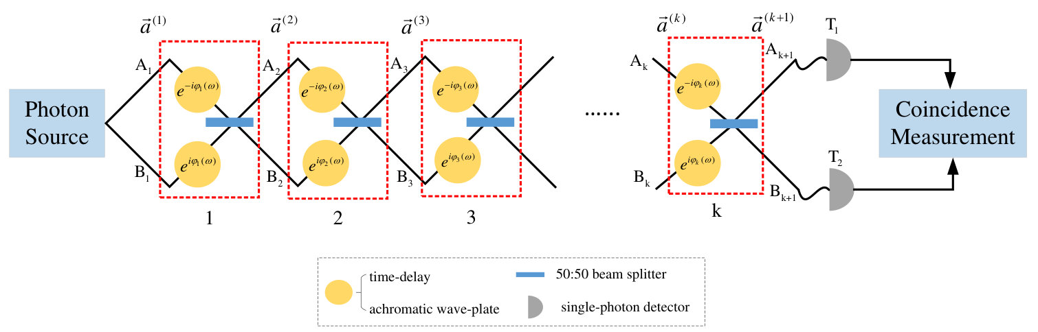 Figure 1
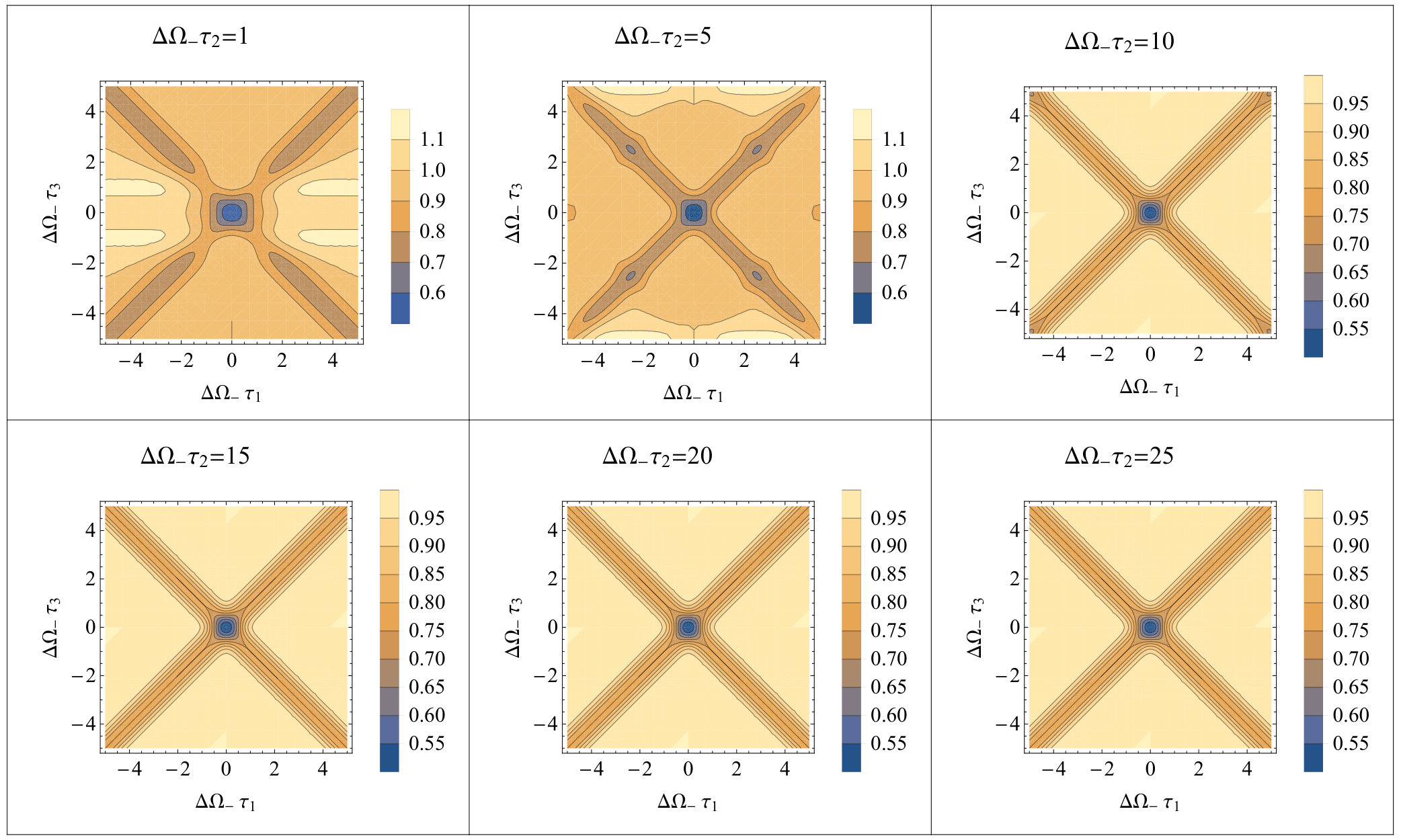 Figure 2
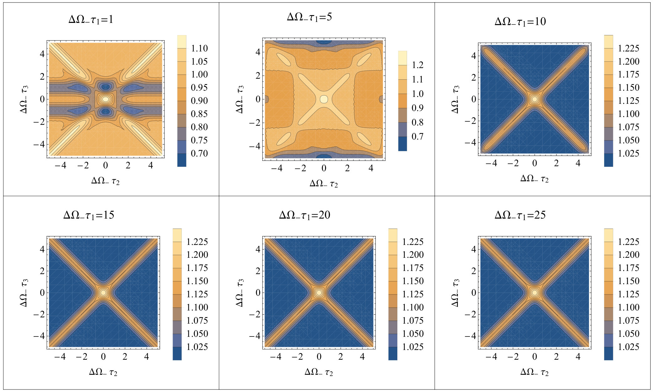 Figure 3
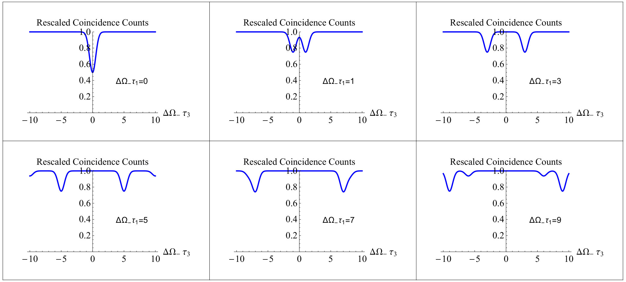 Figure 4
 Figure 5
Peer Reviews
No public reviews on file for this paper yet. If you reviewed it on a platform where reviews are public (OpenReview, ICLR, NeurIPS, ICML), you can paste yours below so the community can read it here.
Videos
No videos yet. Explain this paper in a talk, walkthrough, or lecture? Add one.
Exclusive Hong-Ou-Mandel zero-coincidence point
Yu Yang
School of Aerospace Science and Technology, Xidian University, Xi’an 710126, China
Scuola Normale Superiore, I-56126 Pisa, Italy
Luping Xu
Corresponding Author: [email protected]
School of Aerospace Science and Technology, Xidian University, Xi’an 710126, China
Vittorio Giovannetti
NEST, Scuola Normale Superiore and Istituto Nanoscienze-CNR, I-56127 Pisa, Italy
Abstract
A generalized multi-parameter Hong-Ou-Mandel interferometer is presented which extends the conventional “Mandel dip” configuration to the case where a symmetric biphoton source is used to monitor the contemporary presence of independent time-delays. Our construction results in a two-input/two-output setup, obtained by concatenating 50:50 beam splitters with a collection of adjustable achromatic wave-plates. For and explicit examples can be exhibited that prove the possibility of uniquely linking the zero value of the coincidence counts registered at the output of the interferometer, with the contemporary absence of all the time-delays. Interestingly enough the same result cannot be extended to . Besides, the sensitivity of the interferometer is analyzed when the time-delays are affected by the fluctuations over time-scales that are larger than the inverse of the frequency of the pump used to generate the biphoton state.
pacs:
42.50.-p, 03.67.-a
I Introduction
The Michelson interferometer MI1 ; MI2 , the Hong-Ou-Mandel (HOM) interferometer HOM1 ; HOM2 ; HOM3 ; HOM4 ; HOM5 , and the Mach-Zehnder interferometer (MZI) MZI1 ; MZI2 ; MZI3 ; MZ04 ; MZ01 ; MZ02 ; MZ1 are examples of two-input/two-output set-ups which have been extensively used to study two-photon quantum interference effects, with applications in parameter estimation problems, such as phase estimation in the quantum radar QR , or coordinates estimation in quantum positioning system Bahder:2004 . In these schemes a minimum (or a maximum) in the coincidence counts recorded at the output of the device is typically associated with the case where no relative delays affect the propagation of the photons along the two optical paths of the set-up. In the HOM interferometer this correspondence yields the celebrated “Mandel dip” where, given a symmetric input biphoton (BP) source BIPHOTON0 ; BP-CP-STATE ; BIPHOTON1 ; BIPHOTON2 ; BIPHOTON3 , a zero-coincidence signal can be uniquely linked to the absence of asymmetries in the signal propagation. Generalization of this effect to more than one parameter are naturally provided by MZIs MZI1 ; MZI2 ; MZI3 ; MZ04 ; MZ01 ; MZ02 ; MZ1 where, exploiting the presence of two 50:50 BS, one can in principle monitor two independent time-delays with a single coincidence measurement. It turns out however that for these settings the zero-coincidence event does not exclusively correspond to the contemporary absence of the two delays unless MHOM one includes the presence of an achromatic quarter wave-plate ACHRO1 ; ACHRO2 ; ACHRO3 . Unlike the standard wave-plates, this optical element provides a constant phase shift independent with the wavelength of the incoming light, typically achieved by using two different birefringent crystalline materials balancing the relative shift in retardation over the wavelength range. As shown in Ref. MHOM by inserting it inside the MZI, one can effectively force an exact swap between the symmetric and anti-symmetric components of the spectral wave function of the propagating biphoton signal, restoring the one-to-one correspondence between the HOM zero-coincidence point event and the contemporary absence of the delays in the configuration.
Aim of the presented paper is to study the possibility of extending this result to the case of time-delay parameters. More specifically, we consider a generalized two-input/two-output interferometer formed by concatenated 50:50 BSs and independent time-delay parameters , , , , where with the help of a collection of properly setting achromatic phase-shifts, we try to identify what we dub an exclusive HOM zero-coincidence point event, i.e. a one-to-one correspondence between the zero value in the coincidence counts registered at the output of the interferometer and the contemporary absence of all the time-delays in the scheme. After stating this problem in the rigorous mathematical terms, we observe that while it is explicitly solvable for and (the solutions for and being associated with the results of Refs. HOM1 and MHOM respectively), it admits no solution for , a peculiar behavior which is probably associated with some accidental symmetries. In the second part of the manuscript we study the sensitivity of the scheme in the presence of random fluctuations with respect to the time-delay parameters , , , showing that the effectiveness of the achromatic phase-shifts is strongly affected by such noisy events.
The manuscript is organized as follows: in Sec. II we introduce the setup, setting the notations and introduce a necessary and sufficient condition for the existence of an exclusive HOM zero-coincidence point for the case of time-delay parameters. In Sec. III we hence specify our attentions to and showing that in the first case no solution can be find and presenting instead explicit solution for the second. Moreover some comments for the case is proposed to complete our discussions. In Sec. IV we finally study the sensitivity of the scheme under fluctuating the time-delay parameters. This manuscript finally ends with Sec. V where we present our conclusions and comments on the possible applications to sensing procedures.
II Exclusive HOM zero-coincidence point
Here we propose the scheme and introduce the related notations. More importantly a formal definition of the exclusive HOM zero-coincidence point is presented.
II.1 Scheme structure
Consider the two-input/two-output ports device shown in Fig. 1 which registers the coincidence events at the detectors and associated with a frequency correlated, symmetric biphoton (BP) source BIPHOTON0 ; BP-CP-STATE ; BIPHOTON1 ; BIPHOTON2 ; BIPHOTON3 . As schematically depicted in Fig. 1, the setup is obtained by concatenating modules (red dashed rectangles), labelled by the progressive index , each containing the optical elements that introduce the opposite phase-shifts and in the lower and upper paths in this generalized interferometer respectively, and a 50:50 beam splitter (BS) that coherently mixes them. Reviewing the original HOM configuration, the phase-shifts , , , are assumed to be linked to the time-delays , , , , which in the following will be treated as the independent variables. Furthermore along the lines detailed in Ref. MHOM we also allow for the presence of achromatic wave-plates ACHRO1 ; ACHRO2 ; ACHRO3 that add the frequency independent contributions , , , that we shall use as tunable knobs of the device, writing
[TABLE]
the value of being set equal to zero without the loss of generality as it introduces an irrelevant global phase to the final state of the emerging photons, see below.
Under the above premises, the aim of our analysis is to verify whether it is possible to identify what we dub an exclusive HOM zero-point configuration, i.e. a special assignment of the parameters capable to ensuring that a null value for the coincidence counts at and uniquely corresponds to the case where all the temporal delays of the setup are exactly equal to zeros, i.e.
[TABLE]
For a solution of the above problem is provided by the “Mandel dip” HOM1 . For instead the existence of an exclusive HOM zero-coincidence point follows by the results of Ref. MHOM which achieves (II.1) by employing . In what follows, we shall extend this construction to the larger values of : interestingly enough we observe that for no solution can be found, while for special choices of exist so that (II.1) holds true.
II.2 A necessary and sufficient condition for the symmetric BP state
To set the problem in the rigorous mathematical terms, let us introduce the annihilation operators describing a photon of frequency that enters the -th module of the device along the input path ( denotes the path () respectively) and fulfilling Canonical Commutation Rules (CCR): , where and being the Kronecker and Dirac deltas respectively. The associated output counterpart that is also the input bosonic annihilation operator in the -th module, is connected with by the -th module via the following linear transformation
[TABLE]
with
[TABLE]
where matrix being defined by the phase-shifts introduced in Eq. (1). Therefore, the input-output mapping from the first module to the -th module can now be expressed in the compact form
[TABLE]
with the matrix defined as
[TABLE]
Consider hence the following frequency-correlated biphoton pure state BIPHOTON0 ; BP-CP-STATE ; BIPHOTON1 ; BIPHOTON2 ; BIPHOTON3 as the input state of the setup
[TABLE]
where is the multi-mode vacuum state, and where represents a complex amplitude probability distribution on which for the moment we make no assumptions apart from the normalization condition . Following the principle of coincidence measurement MANDELBOOK , we express the coincidence counts as
[TABLE]
where is the amplitude of electromagnetic field at detector , and where represents the output state emerging from the interferometer associated with the input state . The former one can be obtained by using (9) to express in terms of the corresponding output-mode operator obtaining
[TABLE]
which is inserted into (14) gives us
[TABLE]
Expanding Eq.(II.2) we observe that it contains two kinds of contributions: the first contains the terms where both photons belong to a same output port of the interferometer (either or ) and gives explicitly no contribution to (15); the second instead contains all the terms where one photon in and another one in and which can actively contribute to . Its analytic expression is given by
[TABLE]
where is the new biphoton amplitude that we can write as
[TABLE]
where in the last line we use the symmetric and antisymmetric components of the input distribution
[TABLE]
and introduce the functions
[TABLE]
that correspond respectively to the permanent BATHIA and determinant of the matrix N_{k}(\omega,\omega^{\prime}):=\left(\begin{array}[]{cc}A_{k}(\omega)&B_{k}(\omega^{\prime})\\ C_{k}(\omega)&D_{k}(\omega^{\prime})\end{array}\right) and which exhibit an implicit dependence upon the delays and upon the constant phase shifts , , . Replacing all this into Eq. (15) we finally get
[TABLE]
where in the second line we separate the symmetric and antisymmetric contributions of . The above expression makes it evident that a zero value of coincidence counts can be obtained if and only if the following conditions get satisfied for all and ,
[TABLE]
In particular under the simplifying hypothesis of an input BP state that has a symmetric amplitude analogous to those analyzed in Ref. MHOM , i.e.
[TABLE]
Eq.(26) implies a simple necessary and sufficient condition for having a zero-coincidence counts, i.e.
[TABLE]
which in the following we shall adopt to study the problem (II.1) – being the domain where is supported.
III Multi-parameter HOM zero-coincidence point
From the discussion of Sec II, the presence of a zero value in the coincidence counts when feeding the apparatus with a symmetric biphoton state is related with the possibility of nullifying the function for all points in the support of which, without the loss of generality hereafter we shall assume to be the full frequency domain. As for the scheme defined by a single modulus (), Eqs. (12) and (II.2) reduce to
[TABLE]
Therefore, for all if and only if . Under this assumption we get
[TABLE]
which corresponds to the standard result of coincidence counts observed in the conventional HOM interferometer HOM1 exhibiting as an exclusive HOM zero-coincidence point (“Mandel dip”).
A less non trivial configuration is already obtained in the case of modules which was studied in Ref. MHOM . Here Eqs. (12) and (II.2) yield
[TABLE]
and
[TABLE]
which for gives \mbox{Perm}_{2}(\omega,\omega^{\prime})\Big{|}_{\tau_{1}=\tau_{2}=0}=\cos\theta_{2}. Accordingly from Eq. (28) it follows that we can have by setting . Most importantly under this condition (39) becomes
[TABLE]
for which only can ensure the fulfillment of Eq. (28). Hence also in this case we can conclude that the scheme exhibits an exclusive zero-coincidence point (II.1) under the special setting MHOM .
III.1 Absence of the exclusive zero-coincidence point for modules
Now we consider the case with respect to modules, under this condition Eqs.(12) and (II.2) yield
[TABLE]
and
[TABLE]
where , for . Recalling (1) one can easily verify that for Eq. (45) reduces to
[TABLE]
which can be forced to zero by taking one (or both) of the two phase shifts and equal to an integer multiple of . Interestingly enough none of these settings provide an exhaustive zero-coincidence point (II.1) for the scheme. For instance assuming we get
[TABLE]
which besides admits zero value as all the points proportional to – in the case where the same hold for proportional to . On the contrary for we have
[TABLE]
which instead admits zero value for all points proportional to – the same result also when .
III.2 Exclusive zero-coincidence point for modules
The presence of exclusive zero-coincidence solutions is restored for . Analytically Eqs.(12) and (II.2) get replaced by
[TABLE]
and
[TABLE]
where adopting the same simplifying notation introduced in Eq. (45). For , the above expression reduces to
[TABLE]
We notice that taking for instance the above expression can be forced to zero. Yet, one can easily verify that under this condition we do not get an exclusive HOM zero-coincidence point as also nullifies for e.g. proportional to the vector . Similar discussion holds also for the cases where either and , or where instead , . Excluding these cases, e.g. requiring , we can still force Eq. (III.2) to zero by fixing the achromatic phases to fulfill the identity
[TABLE]
We claim that under these conditions the model exhibits indeed an exclusive zero-coincidence point. For this purpose we observe that from Eq. (28) it follows that a necessary condition to have zero value for coincidence counts is to nullify the real part of for all possible choices of and in the domain, i.e.
[TABLE]
Restricting the analysis to the case the above equation yields hence the following condition
[TABLE]
which must hold for all if we want to get : as shown in Sec. III.2.1 below however this condition can only be achieved when , which when inserted into (III.2) finally leads to identify as the unique zero-coincidence point of the model.
III.2.1 Existence of the exclusive zero-coincidence point
Here we explicitly show that for proper choices of as in Eq. (54), Eq. (III.2) admits as unique solution, hence proving that for we can have the exclusive zero-coincidence point condition (II.1). Firstly, let us observe that we can exclude the cases with . Indeed under the condition of Eq. (III.2) yields
[TABLE]
which, considering that we are discussing the case where and Eq. (54) holds true, can be satisfied for all only taking . However now we shall have so that Eq. (III.2) becomes
[TABLE]
which is null for all and only when we have also . Secondly, considering the case where at least one among and is different from zero. Under this condition it is convenient to rewrite Eq.(III.2) as
[TABLE]
with
[TABLE]
and
[TABLE]
We now observe that if at least one among and is different from zero, then is an oscillating function of characterized by two independent frequencies and . On the contrary in general admits four different frequencies (explicitly given by ) apart from the special degenerate cases where we have either , or , which both admits 3 independent frequency values. The only possibility to fulfill (59) (and hence (III.2)) is that in the above configurations, the multiplicative coefficients of such frequency terms help us to reduce the effective number of frequencies of to two. By looking at Eq. (61) however, this can only happen in the degenerate cases. For instance, for by taking we can reduce Eq.(61) to
[TABLE]
Still we notice that in this case it is impossible to obtain the identity (59) due to the mismatching between the prefactor of and the prefactor of .
III.3 Exclusive zero-coincidence point for
From the previous subsections it is clear that as increases determining the condition under which Eq. (II.1) can be fulfilled becomes harder and harder. In particular the absence of a solution for suggests that the problem cannot be solved by induction. Still we suspect that for large enough , the possible combinations of , , ensuring the condition
[TABLE]
will increase. For instance in passing from to we go from a very constrained set solutions where one among and is forced to be an integer multiple of (see Eq. (46)) to (54) which allows , and to span over a dense set of possibilities. Exploiting this increased freedom in the selection of , , it is reasonable to assume that among them it would be possible to find a special assignment to force Eq. (II.1). Accordingly it is expected that this problem is always solvable for (possibly excluding some isolated and pathological cases).
IV Sensitivity to fluctuations
To get a concrete example we now specialize the analysis under the assumption of a BP input state (14) with Gaussian two-mode spectral function of the form
[TABLE]
with the following normal distributions
[TABLE]
which locally assigns to each photon an average frequency with spread . In the limit , Eq. (64) approaches the frequency-entangled biphoton state emerging from an ideal Spontaneous Parametric Down Conversion (SPDC) source pumped with a laser of mean frequency , e.g. BIPHOTON0 ; BIPHOTON1 ; BIPHOTON2 ; BIPHOTON3 and references therein; for instead it corresponds to two uncorrelated (unentangled) single-photon packets; while finally for it mimics the properties of an entangled state emitted by a difference-beam (DB) source BP-CP-STATE . Under the condition (64) it follows that the associated coincidence counts (II.2) can be expressed as the sum of two contributions,
[TABLE]
where the whole dependence upon , , is only carried by which, as a function of , , , exhibits a series of fast oscillations with frequency , and where depends instead only upon the spectral width which determines the spread of the frequency mismatch of the two input photons (see Sec. IV.1 for details). The special decoupling enlightened in Eq.(66) implies that in the presence of fluctuations of the delays , , , the functional dependence of upon is washed away. To see this assume that each of these parameters fluctuates randomly and independently on intervals which are much larger than the inverse of the mean biphoton frequency but smaller than the inverse of the associated local spread (i.e. ). In this case the result of coincidence counts registered at the output of the set-up is effectively provided by the coarse graining counterpart of MHOM , i.e.
[TABLE]
Now from Eq. (66) it follows that
[TABLE]
(see again Sec. IV.1 for a formal derivation of these identities that holds for arbitrary values of ). Eq.(68) makes it explicit the fact that the achromatic shifts , , , while enforcing the exclusive zero-coincidence point condition (II.1), become inconsequential in the presence of fluctuations of the time-delays. For this is a direct consequence of the fact that in the original HOM scheme one has
[TABLE]
the contribution being explicitly zero after the coarse graining – of course this is also the only case which exhibits a zero-coincidence point without achromatic phase shifters. For the case instead we get MHOM
[TABLE]
while, as explicitly discussed in Appendix A, for we get
[TABLE]
IV.1 Effect of the coarse graining
Here we present a derivation of Eq. (68) for arbitrary . We start observing that from Eq. (12) it follows that the various matrix elements of can be expressed as
[TABLE]
where the summation runs over the set of -long vector formed by the sequences of , where , and where finally , , , and are the complex parameters of modulus which are independent from the phase . Accordingly we can write
[TABLE]
where in the second identity we introduced the quantities
[TABLE]
and used Eq. (1) to write
[TABLE]
with and . We now split the summation of Eq. (IV.1) into term and term respectively, i.e.
[TABLE]
with
[TABLE]
where we use the fact that and . Taking the modulus we have
[TABLE]
which is further expressed as
[TABLE]
with being a function that only depends upon but bares no functional dependence neither upon nor upon , while being a sum of contributions which exhibit the phase-shift terms that have a non-trivial dependence upon . Specifically,
[TABLE]
with and being the subsets formed by the couples such that and respectively (notice that they have zero overlap). Using Eq. (80) to compute the coincidence counts we hence arrive to Eq. (66) via the identification
[TABLE]
and
[TABLE]
We used (64) to split the integral in terms of the variable and , hence Eq. (IV.1) is given by
[TABLE]
with the vector being explicitly non-zero. As anticipated in the main text before, depends explicitly upon and . Furthermore we notice that under coarse graining we have
[TABLE]
where in the first identity we used the fact that since we assume , the integral is performed over intervals of length which is much shorter than and . Inserting this into (IV.1) we can thus conclude that
[TABLE]
which proves the second identity of Eq. (68). The first one follows along the same line by observing that according to Eq. (IV.1) the right-hand-side term of (IV.1) is given by a finite summation of terms which are either constant or have the following dependence on ,
[TABLE]
with being some non-zero vectors, we notice that the values of , , and reported in Eqs. (69)–(71) have indeed this structure. Therefore, repeating the same argument used in Eq.(IV.1) in this case we get
[TABLE]
which ultimately leads to
[TABLE]
and hence get the first identity of Eq. (68).
V Conclusion
A generalized multi-parameter HOM interferometer composed by 50:50 beam splitters, different time-delays and achromatic wave-plates has been presented. In the special case with modules, the described setup was employed in Ref. MHOM as a scheme to measure two independent time-delays parameters via the results of coincidence counts at the output. Borrowing directly from the original HOM scheme HOM1 , the idea was to link the uniqueness of a HOM zero-coincidence point attainable when setting , to a way for detecting the non-zero values of and , thereby compensating for them by adding the controllable delays along the interferometric paths. From the results presented at here, it is clear that the same construction can be extended to the case of modules, while this would not be possible for the case of just three modules due to the impossibility of fulfilling the condition (II.1) for . In Ref.MHOM it was also shown how to use the residual functional dependence of the coarse-grained coincidence counts (IV) upon the delays to determine their values. Clearly the same construction can be applied also for larger values of . In particular this can be done for the unlucky case which, in the presence of fluctuations, does not even admits an exclusive HOM zero-coincidence point. As a matter of fact, from Figs.2–3 we notice that fixing , exhibits two symmetric dips as a function of for assigned values of , with a visibility (the ratio between the depth of the minima and the height of the plateau). On the contrary, from Figs.4–5 it follows that for , exhibits instead two symmetric peaks as a function of for assigned values of , with the visibility (the ratio between the maximum value and the height of the plateau). Consider then the case where each of the length-difference of paths , and as , , where is fixed and unknown, the second term is controllable by the experimentalist. One way to recover these parameters could be the following procedure: i) we select to be sufficiently large to ensure that the value to be larger than . Then keeping , we record the values of as a function of , locating the two minima , of Fig.3. This allows us to determine the values of and by observing that and respectively; ii) With this information we now set to get larger than , keeping and start scanning once more with respect to to locate the maxima , of Fig.5, hence the value of can be obtained as .
The Authors acknowledge support from the Grant National Natural Science Foundation of China 61172138, 61573059, 61771371; Aviation Science Foundation Project 20160181004; Shanghai Aerospace Science and Technology Innovation Fund SAST2017-030, and SNS for hosting her.
Appendix A Appendix
As for the modules, of Eq.(66) with respect to and is given by
[TABLE]
with
[TABLE]
The reference list from the paper itself. Each links out to its DOI / PubMed record.
- 1(1) J. Brendel, E. Mohler, and W. Martienssen, Phys. Rev. Lett. 66 , 1142 (1991).
- 2(2) S. Odate, H. Wang, and T. Kobayashi, Phys. Rev. A 72 , 063812 (2005).
- 3(3) C. K. Hong, Z. Y. Ou, and L. Mandel, Phys. Rev. Lett. 59 , 2044 (1987).
- 4(4) T. Kobayashi, et al. , Nat. Photonics 10 , 441 (2016).
- 5(5) A. Lyons, et al. , Sci. Adv. 4 , 5 (2018).
- 6(6) H. Kim, S. M. Lee, and H. S. Moon, Sci. Rep. 5 , 9931 (2015).
- 7(7) Y. Chen, et al. npj Quantum Inform. 5 , 43 (2019)
- 8(8) Z. Y. Ou, X. Y. Zou, L. J. Wang and L. Mandel, Phys. Rev. A 42 , 2957 (1990).