Multiple asymptotics of Kinetic Equations with Internal States
Benoit Perthame, Weiran Sun, Min Tang, Shugo Yasuda

TL;DR
This paper investigates the derivation of macroscopic models from microscopic assumptions in bacterial movement, revealing how different asymptotics lead to classical or flux-limited Keller-Segel equations and introducing new equilibrium equations with singular solutions.
Contribution
It provides a mathematical framework connecting microscopic internal states to macroscopic chemotaxis models, highlighting the impact of response stiffness and adaptation time on resulting equations.
Findings
Derivation of macroscopic equations from microscopic internal states.
Identification of conditions leading to Keller-Segel and flux-limited Keller-Segel models.
Discovery of new equilibrium equations with singular solutions.
Abstract
The run and tumble process is well established in order to describe the movement of bacteria in response to a chemical stimulus. However the relation between the tumbling rate and the internal state of bacteria is poorly understood. The present study aims at deriving models at the macroscopic scale from assumptions on the microscopic scales. In particular we are interested in comparisons between the stiffness of the response and the adaptation time. Depending on the asymptotics chosen both the standard Keller-Segel equation and the flux-limited Keller-Segel (FLKS) equation can appear. An interesting mathematical issue arises with a new type of equilibrium equation leading to solution with singularities.
Click any figure to enlarge with its caption.
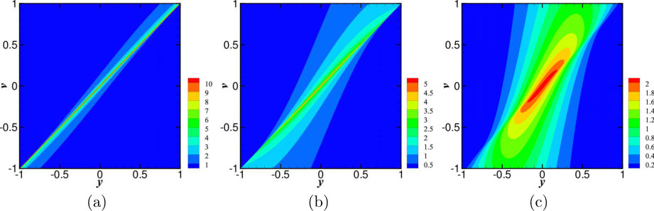 Figure 1
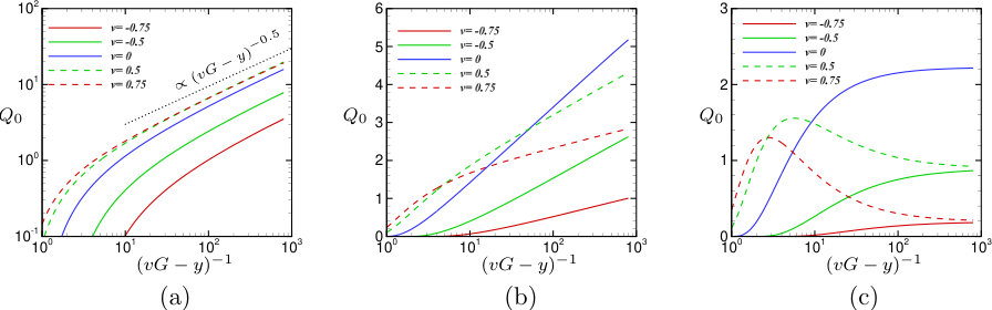 Figure 2
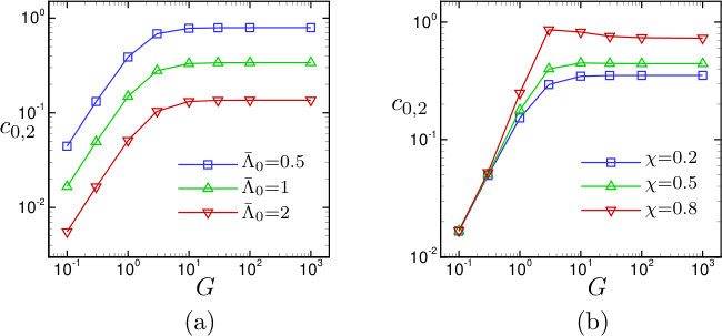 Figure 3
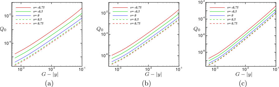 Figure 4
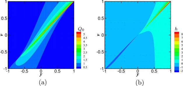 Figure 5
| =2.0 | =0.5 | ||||
|---|---|---|---|---|---|
| 200 | 9.1 | 1.2 | 8.1 | 4.2 | |
| 400 | 2.2 | 2.9 | 5.8 | 2.5 | |
| 800 | 5.4 | 6.9 | 3.4 | 1.3 | |
| 1600 | 1.1 | 1.4 | 1.5 | 5.5 | |
Peer Reviews
No public reviews on file for this paper yet. If you reviewed it on a platform where reviews are public (OpenReview, ICLR, NeurIPS, ICML), you can paste yours below so the community can read it here.
Videos
No videos yet. Explain this paper in a talk, walkthrough, or lecture? Add one.
Multiple asymptotics of Kinetic Equations with Internal States
Benoit Perthame
Sorbonne Université, CNRS, Université de Paris, Inria, Laboratoire Jacques-Louis Lions UMR7598, F-75005 Paris
,
Weiran Sun
Department of Mathematics, Simon Fraser University, 8888 University Dr., Burnaby, BC V5A 1S6, Canada
,
Min Tang
Institute of natural sciences and department of mathematics, Shanghai Jiao Tong University, Shanghai, 200240, China
and
Shugo Yasuda
Graduate School of Simulation Studies, University of Hyogo, 650-0047 Kobe, Japan
Abstract.
The run and tumble process is well established in order to describe the movement of bacteria in response to a chemical stimulus. However the relation between the tumbling rate and the internal state of bacteria is poorly understood. The present study aims at deriving models at the macroscopic scale from assumptions on the microscopic scales. In particular we are interested in comparisons between the stiffness of the response and the adaptation time. Depending on the asymptotics chosen both the standard Keller-Segel equation and the flux-limited Keller-Segel (FLKS) equation can appear. An interesting mathematical issue arises with a new type of equilibrium equation leading to solution with singularities.
Key words and phrases:
flux limited Keller-Segel system; chemotaxis; drift-diffusion equation; asymptotic analysis; kinetic transport theory
2010 Mathematics Subject Classification:
35B25, 35Q20, 35Q84, 35Q92, 92C17
1. Introduction
Chemotaxis is the movement of bacteria in response to a chemical stimulus. Individual bacteria moves by alternating forward-moving runs and reorienting tumbles. The velocity jump model has been proposed to describe the switching between these two states, in which the two processes, run-to-tumble and tumble-to-run, are modelled by two Poisson processes. The frequencies of these two poisson processes are determined by intracellular molecular biochemical pathway. Therefore, to study the chemotaxis behaviour quantitatively, it is crucial to understand the response of bacteria to signal changes and relate this information to the switching frequency. The mechanism has been well understood for Escherichia coli (E. coli) chemotaxis and other bacteria using similar strategies to move have also been observed ([Duffy97, Hazelbauer12]). In what follows we will focus on the behavior of E. Coli.
It is known that E. coli responds to signal changes in two steps: excitation and adaptation. Excitation is when E. coli rapidly changes the tumbling frequency as it detects external signal changes, while the slow adaptation allows the cell to relax back to the basal tumbling frequency (the frequency when the intracellular chemical reactions are at equilibrium) [JOT]. In the simplest description of the biochemical pathways, a single variable is used to represent the intracellular methylation level. The methylation has an equilibrium level which is a function of extra-cellular chemical concentration. Using as the adaptation rate, the equation for the adaptation process has the form
[TABLE]
The switching frequencies of run-to-tumble and tumble-to-run are determined by both and . The tumbling time can be ignored since it is usually much shorter than the running time, thus one can combine the two successive processes run-to-tumble and tumble-to-run together and assume that once the bacterium stops run it will immediately choose randomly some direction and start running again. Tumbling frequency is used to describe this Poisson process and it depends on the methylation level and its equilibrium .
In order to understand the relation between individual bacteria movement and their population level behaviour, pathway-based kinetic-transport model has been proposed in [ErbanOthmer04, SWOT]. This model governs the evolution of the probability density function of the bacteria at time , position , velocity , and methylation level . The velocity space is for and for (the sphere with radius ). The general form of the kinetic equation is
[TABLE]
where the tumbling term satisfies
[TABLE]
Here is the methylation-dependent tumbling frequency from to and .
The pathway-based kinetic equation in (1.1) is at the mesoscopic level. It can bridge the microscopic (individual) and macroscopic (population) level models by using moment closure or asymptotic analysis [ErbanOth2, SWOT, ST, STY, Xue2]. In this paper, we are interested in building such connections of some macroscopic models with (1.1). Particular attention will be paid to the flux-limited Keller-Segel (FLKS) model. The most standard and popular macroscopic population level model describing the dynamics of the bacteria density is the classical Keller-Segel (KS) model [Patlak, KS1, KS2]. There has been extensive mathematical studies of the KS equation [BBW2015]. Analytically it has been discovered that depending on the cell number, solutions of KS model can either undergo smooth dispersion or blow up in finite time [CW08, BCL09]. The reason that blow-up could happen is because the drift velocity is proportional to the gradient of the external chemicals . Therefore it is not bounded when . This is in discrepancy with reality since the population level drift velocity is expected to saturate when the chemical gradient is large. Hence in [HP09] a more physically relevant FLKS model is proposed, which has the form
[TABLE]
where is the cell density at time and position , is a bounded function in . Unlike the classical KS model, the solution to (1.3) exists globally in time [Chertock, BW2017]. Interesting features of the FLKS are specific stiff response induced unstability and existence of traveling waves (stable or unstable), [PeYa2018, CPY2018].
The classical KS model has been recovered from the kinetic equation (1.1) as diffusion limits, as well as the FLKS [PVW2018]. In [ErbanOthmer04, XO], the authors derived the KS equation by incorporating the linear adaptation. Recently, intrinsically nonlinear signaling pathway are considered [STY, Xue2]. The derivations in [ErbanOthmer04, STY, SWOT, XO, Xue2] are formal and are based on moment closure techniques. When the internal state is not far from its expectation, the moment closure method provides the correct behavior of E. coli on the population level. However, the closeness assumption is only valid when the chemical gradient is small so that the internal states of different bacteria can concentrate and yield the KS equation [SWOT, ST, Xue1]. In general this assumption does not always apply for other scales of the chemical gradient and adaptation time. Our goal is to derive different macroscopic models for different chemical gradient and adaptation time by asymptotic analysis.
We assume that the tumbling frequency depends only on . This assumption is valid for E. coli chemotaxis [SWOT]. Moreover, we use the following linear model for the adaptation
[TABLE]
where gives the characteristic time scale of the adaptation process [ErbanOthmer04]. Introducing a new variable
[TABLE]
and letting , one can rewrite the original model (1.1) as
[TABLE]
In this paper, we only consider the case when is independent of time and is uniform in space. This special case is physically interesting: for E. coli chemotaxis, since is related to the extra-cellular attractant profile by a logarithmic dependency, a uniform corresponds to the exponential environment as in the experiment in [Kalinin]. Let be the constant vector given by
[TABLE]
Let be the characteristic rate of tumbling and the stiffness of the response. We denote
[TABLE]
Then equation (1.6) becomes
[TABLE]
To perform the asymptotic analysis, we introduce the non-dimensional variables
[TABLE]
where , , and are the characteristic length, speed, and time respectively. Then the equation 1.8 is reformulated as
[TABLE]
with the parameters given by
[TABLE]
Since there will be no confusion, in the remainder of the paper we drop the tilde sign for simplicity. The final form of the kinetic equation under consideration is
[TABLE]
Our goal in this paper is to start from (1.10) and systematically derive macroscopic limits from it: assuming is large and , we consider the seamless reorientation by runs and tumbles with different scalings of and . More specifically, we investigate the following three cases:
- I.
Fast adaptation and stiff response: both and are as small as ;
- II.
Very fast adaptation and very stiff response: both and are much smaller than ;
- III.
Moderate adaptation and moderate response, i.e. both and are of .
The common theme in these limits is to decide when the classical KS and the FLKS equations will occur. A brief summary of our result is
- (1)
In Case I, both the hyperbolic model and a FLKS type model can be found. In particular, when the leading order behaviour of the bacteria population satisfies a hyperbolic model, we further consider the motion of its front profile and find a FLKS model in the moving frame. 2. (2)
In Case II, a FLKS type model can be derived. 3. (3)
In Case III the solution will tend to the solution of a classical KS model.
The rest of the paper is organized as follows. In Section 2, we use asymptotic analysis to formally derive the leading-order macroscopic equations from (1.1). Some properties of the leading order distribution are rigorously shown in Section 3. In Section 4, we show numerical results that are consistent with the analytical properties in Section 3. Finally we conclude in Section 5.
2. Formal Asymptotic Limits
In this section we show that both classical and flux-limited Keller-Segel equations can arise in different physical regimes characterized by the stiffness of the chemotactic response and the rate of adaptation. In all the cases considered below we fix as
[TABLE]
2.1. Fast adaptation and stiff response
In this case we assume that
[TABLE]
We also assume that the tumbling frequency has the specific structure
[TABLE]
where is a strictly positive continuous function and is independent of . The space is the collection of continuous and bounded functions on .
Consider the scaled equation
[TABLE]
The leading-order term of is of the form where satisfies
[TABLE]
The existence and uniqueness of such is shown in Theorem 3.1.
Remark 2.1*.*
In Theorem 3.1 we show that is compactly supported on and is strictly positive in . In the rest of the current section, all the integration involving are performed over , although we often write the integration domain as for the sake of simplicity in notation.
Let be the leading-order average velocity given by
[TABLE]
In the case where , by letting one can derive that the leading-order approximate of satisfies a pure transport or hyperbolic equation. More specifically, we have the formal limit
Theorem 2.1**.**
Suppose and satisfies (2.1) together with the assumptions in Theorem 3.1. Suppose the average velocity defined in (2.4) is nonzero. Let be the non-negative solution to (2.2). Suppose in . Then and satisfies the hyperbolic equation
[TABLE]
Proof.
Since (2.2) is a linear equation, we can pass and obtain as a non-negative solution to the steady-state equation such that
[TABLE]
By the uniqueness shown in Theorem 3.1, is a multiple of with a coefficient . The conservation law associated with (2.2) and has the form
[TABLE]
The limiting equation (2.5) is obtained by passing and using that . ∎
To observe nontrivial diffusive behaviour from equation (2.2), we make a change of variable such that
[TABLE]
where again is the average speed defined in (2.4). Physically speaking, we consider the motion of the front profile of . Now we let . Then the equation for reads
[TABLE]
Before showing the formal limit for , we prove a lemma of the classical entropy-estimate type:
Lemma 2.1**.**
Let be the operator defined as
[TABLE]
Let be the unique solution in (2.3). Then for any that makes sense of all the integrals and satisfies that
[TABLE]
we have
[TABLE]
Note that a particular case for (2.8) to hold is when .
Proof.
The proof follows from a direct calculation. Indeed, by integration by parts,
[TABLE]
where condition (2.8) is used to guarantee that the boundary terms vanish in the integration by parts. Using the equation for , we have
[TABLE]
The equal sign holds only when is independent of . ∎
Equipped with Lemma 2.1, we show the formal asymptotic limit of (2.6) in the following theorem:
Theorem 2.2**.**
Let be the non-negative solution to (2.6) and such that
[TABLE]
for some . Then and satisfies the drift-diffusion equation
[TABLE]
where the diffusion coefficient and drift velocity are given by
[TABLE]
*Moreover, is strictly positive. *
We conjecture that is bounded in , thus rising again a FLKS type equation. A possible route toward a proof is as follows. We write
[TABLE]
and it remains to establish that is uniformly bounded in in . Numerics sustain this boundedness, see Fig. 5.
Proof.
First, we use the same argument as in Theorem 2.1 to deduce that there exists such that and in . Next, the conservation law for (2.6) reads
[TABLE]
By the definition of and , we have
[TABLE]
Hence (2.12) can also be written as
[TABLE]
Then we can re-write equation (2.6) as
[TABLE]
By Theorem A.1, we apply the pseudo-inverse of and obtain that
[TABLE]
Note that every term on the right-hand side of the above equality is well-defined since the terms inside all satisfy the orthogonality condition given in (A.2). By the limit we have
[TABLE]
Hence, it formally holds that
[TABLE]
Inserting such limit in the limiting form of the conservation law in (2.12) gives (1.3) with and satisfying (2.10) and (2.11) respectively.
Finally, we show that is a positive definite matrix. To this end, denote
[TABLE]
or equivalently,
[TABLE]
Then for any arbitrary ,
[TABLE]
Hence,
[TABLE]
By Lemma 2.1, if we multiply to and integrate in , then
[TABLE]
This shows is non-negative and the equal sign of the above inequality holds only when is independent of . Now we show that for any independent of , the quantity must depend on . Hence the strict positivity of must hold. To this end, suppose on the contrary that there exists independent of and such that . Then
[TABLE]
which, by the definition of simplifies to
[TABLE]
Since is independent of , the only solution to such equation is and . Hence for any . This proves the strict positivity of the diffusive coefficient matrix . ∎
In order to justify that (1.3) is indeed a flux-limited Keller-Segel equation, ideally we want to show that the drift velocity is generally nonzero, it is uniformly bounded in the chemical gradient and vanishes when approaches zero. In what follows we show that these properties are satisfied in the special case where is a constant. In Section 4 we give some numerical evidence that is uniformly bounded in even when depends on .
Lemma 2.2**.**
Suppose is a constant. Then the drift velocity satisfy that
(a) is nonzero.
(a) is bounded for all . Moreover, as .
Proof.
(a) Since is a constant, must satisfy the symmetry condition (3.4) in Theorem 3.1. Hence . Moreover, we have the relation since satisfies the equation
[TABLE]
The drift velocity is now reduced to
[TABLE]
We want to show that as a function in is not zero. To this end, we integrate (2.3) in . This gives
[TABLE]
Since is compactly supported on , one must have
[TABLE]
Since is not a zero function in , we deduce that is not a zero function in either. Since , there exists such that
[TABLE]
(b) With the assumption that is a constant, we have derived the simplified form of in (2.15). Then
[TABLE]
Hence is uniformly bounded in . Since is continuous and , we have
[TABLE]
Hence vanishes as approaches zero. ∎
2.2. Very fast adaptation and very stiff response
In this subsection we show a second scaling where flux-limited Keller-Segel equations can also arise. We consider the regime that combines the scalings in [PTV2016] and [PVW2018]. In particular, let
[TABLE]
Then the scaled equation becomes
[TABLE]
Assume that satisfies the same condition as in [PVW2018] such that
[TABLE]
where is a positive constant and . Denote as the space of probability measures in . The formal asymptotic limit is
Theorem 2.3**.**
Let be the solution to (2.16) with satisfying (2.17). Suppose there exists such that as probability measures. Then
[TABLE]
Moreover, satisfies the flux-limited Keller-Segel equation
[TABLE]
with
[TABLE]
Proof.
Passing in (2.16) gives the equation for as
[TABLE]
By the non-negativity of (and a similar argument as in Theorem 3.1 showing its support), we have
[TABLE]
Hence, there exists such that
[TABLE]
The conservation law associated with (2.16) is
[TABLE]
To derive the limit of the -term, we multiply (2.16) by and integrate in . This gives
[TABLE]
Passing and applying (2.20), we have
[TABLE]
where satisfy (2.19). ∎
Note that in general the drift velocity is non-zero. If with , then by the rotational invariance, is along the direction of the chemical gradient . Moreover, it is bounded for all as long as is a bounded function. Similar as in the proof of Lemma 2.2, for being continuous, we have as . These observations justify that (2.18) is of the flux-limited Keller-Segel type.
2.3. Moderate Adaptation and Moderate Response
The classical Keller-Segel equation can also be derived from kinetic equations with the internal state. The particular scaling is for a slow adaption and a moderate gradient where
[TABLE]
The scaled equation is
[TABLE]
In this case we only need to require that , in particular, it does not have to satisfy the specific form in (2.1). The formal asymptotic limit is
Theorem 2.4**.**
Suppose and for all . Let be the non-negative solution to (2.21). Suppose there exists such that as probability measures. Then and satisfies the Keller-Segel equation
[TABLE]
with the diffusion coefficient and drift velocity given by
[TABLE]
Proof.
The conservation law associated with (2.21) is
[TABLE]
We apply the Hilbert expansion for equation (2.21). Write formally
[TABLE]
Then the leading order satisfies
[TABLE]
Hence is independent of . The next order in equation (2.21) gives
[TABLE]
The solvability condition requires that
[TABLE]
Since is independent of , this reduces to
[TABLE]
By the non-negativity of , we must have
[TABLE]
Hence, concentrates at , that is, there exists such that
[TABLE]
Divide (2.21) by , and then multiply by and integrate in . We obtain
[TABLE]
Passing , we formally obtain that
[TABLE]
Apply such limit in (2.22) gives the regular Keller-Segel where the drift velocity is linear in the chemical gradient as long as . ∎
Remark 2.2*.*
One can consider a fourth case with slow adaptation and stiff response where
[TABLE]
The scaled equation is
[TABLE]
If we change the variable to , then the model becomes
[TABLE]
A special choice of with will give rise to a pure diffusion equation, as can be seen by letting to be a constant in Case III. The case of actual interest for further studies is of course when the tumbling rate takes the general form as in section 2.3.
3. Existence and Properties of
In several scaling limits, the equilibrium occurs as the solution of the eigenfunction problem
[TABLE]
Here, we prove existence and uniqueness of assuming that may depend continuously on and satisfies, for two constants , the bounds
[TABLE]
We also derive some basic properties of . The precise statement is
Theorem 3.1** (Existence and regularity of ).**
Suppose is continuous and satisfies (3.3), then there exists a unique probability solution of equation (3.1). Moreover, , is compactly supported on , strictly positive on and satisfies
(a) and is Lipschitz continuous in compact subsets of ;
(b) If , then blows up at the diagonal , with a rate no less than ;
(c) If , then ;
(d) If , then blows up at the diagonal at most as
[TABLE]
Furthermore, for fixed, only depends on in the direction . In the special case where is an even function in , is even in ,
[TABLE]
Remark 3.1*.*
Additionally, one can check that for the blow-up is at least logarithmic and for , the blow-up is at most logarithmic.
Proof.
The proof is organized as follows. We build a probability solution by a time evolution method and denote integration by rather than . Then, we prove that such solution satisfies the announced properties. Finally we prove uniqueness.
Compact Support First we show that any probability solution to (3.1) must be compactly supported on . Indeed, integrating (3.1) in gives
[TABLE]
Therefore, there exists a constant such that
[TABLE]
We claim that by the following observations:
[TABLE]
For any , repeating the above argument, we have
[TABLE]
Therefore for any which implies if . Similar argument applies when . Hence is compactly supported on .
Existence Second, we show the existence of a solution of (3.1) with a support contained in . To this end, let be arbitrary and consider the evolution equation
[TABLE]
where the initial data satisfies
[TABLE]
The global existence of a non-negative solution to (3.5) is a classical matter. Moreover,
[TABLE]
We can show that also has a support included in . To this end, let be a non-negative function such that
[TABLE]
Because we always have , multiplying to (3.5) and integrate in gives
[TABLE]
Using the compact support property for , we conclude that
[TABLE]
The compact support property follows.
Now, consider the family of probability measures on . Being compactly supported, it is tight. Therefore, there exists a probability measure such that, after extraction of a subsequence,
[TABLE]
Take the limit in equation (3.5), we have
[TABLE]
Define the probability measure by
[TABLE]
then it satisfies the equation (3.1) with support contained in .
The next steps are to prove that this measure is an function with the announced properties.
Some general bounds on ** In the sequel, we will make use of the following representation of any weak solution of (3.1). We first deal with the values of and such that . For to be chosen later, we multiply equation (3.1) by and use the chain rule to obtain**
[TABLE]
The choices and yield successively
[TABLE]
[TABLE]
Integrating for (in fact and we keep this bound which is more convenient for later computations), we find
[TABLE]
[TABLE]
does not carry mass on the diagonal.** We conclude from (3.9) that is an function away from the diagonal where . However, this is not enough because our arguments below require that does not carry mass on the diagonal. To do so, decompose with a measure supported by and . Inserting this decomposition in the equation, we find**
[TABLE]
Since is independent of , its restriction on as a measure is zero. Hence .
Bound ** We estimate on the sets and separately since the diagonal does not carry mass. For , we integrate inequality (3.9) in and obtain**
[TABLE]
The inner integral in is bounded as
[TABLE]
and thus , for , we conclude, using as a constant which may change from line to line and depend on , , , that
[TABLE]
Therefore, we find
[TABLE]
As a first step, we now show that . To this end, the contribution to the -norm of on satisfies, using Jensen’s inequality,
[TABLE]
where we have used the fact that is a probability measure and the last inequality holds because
[TABLE]
The estimate for the integral where is similar. Combining the two parts over and , we conclude that .
Building on the -bound of we can now show that . To this end, use (3.11) and the Cauchy-Schwarz inequality,
[TABLE]
since
[TABLE]
The -bound of follows in a similar way and the details are omitted. Combining these two parts, we obtain that .
is Lipschitz continuous away from the diagonal.** We now prove continuity of and thus we also obtain that for except for the diagonal points . Such behaviour of is depicted in the numerical results in Section 4. The proof for continuity uses the representation formula for the solution. We re-write the -equation as**
[TABLE]
Away from the diagonal , the exponential term is smooth in and continuous in , and the right-hand side is in , which implies that is Lipschitz continuous on every compact set in .
Strict positivity of and ** Again we first deal with the values of and such that . Using inequality (3.8) one has**
[TABLE]
**As before we begin with the inner integral and estimate it, for , as **
[TABLE]
where is again a constant depending on , , which changes from line to line. This yields
[TABLE]
The same calculation, for gives,
[TABLE]
Finally we arrive at
[TABLE]
The strict positivity of then follows from the lower bound on and (3.8).
Upper bound for ** Using the upper bound on and (3.9), we conclude that for **
[TABLE]
and a similar inequality for concludes the points (c) and (d).
Uniqueness, dependency and symmetry** Finally, we show that a probability solution to (3.1) must be unique. Suppose instead there are two probability solutions, denoted as and . From the steps above, these are functions. To avoid the difficulty that , vanish near the boundary , we introduce**
[TABLE]
The main advantage of is the uniform boundedness given by
[TABLE]
Such bound is elusive a-priori for , which renders integration by parts involving invalid. Note that by the linearity of (3.1), is also a normalized non-negative solution which satisfies all the properties shown above. In particular, is strictly positive in \big{(}(-|G|,\,|G|)\times\mathbb{V}\big{)}. The uniqueness is shown by a similar argument as proving the positivity of in Theorem 2.2. In particular, to make use of the entropy-type estimate, we multiply to the -equation and integrate in . Since are both solutions to (3.1), we apply the same estimate as in the proof of Lemma 2.1 and obtain that
[TABLE]
Therefore, is independent of . Hence there exists a function such that
[TABLE]
Inserting such relation in the -equation gives
[TABLE]
We can now use the -equation to derive that
[TABLE]
This implies that is a constant function in . If we denote it as , then . By the normalization conditions for both , we get , which further implies that , therefore the uniqueness.
From uniqueness, the symmetry in (3.4) follows immediately since is also a non-negative and normalized solution to (3.1). To show that depends only on , we remark that the solution in , with the direction of can be extended to a solution in dimension in (independent of the orthogonal directions to ) and this provides the unique -dimensional solution. ∎
4. Numerical illustration on
We now numerically illustrate the properties established previously on the solution of equation (3.1) with which means . We also make the connection with the coefficients found for the continuum FLKS limits and compute the flux defined by (2.11).
In order to calculate , we first solve the leading order equation (3.1) to obtain , and then we solve the following equation of the next order by using , i.e.,
[TABLE]
with the constraint
[TABLE]
The flux is finally obtained by the integration of the solution such that
[TABLE]
We note that in the case when is a constant, i.e., , the flux is directly calculated from by
[TABLE]
4.1. Numerical Scheme
We consider the lattice mesh system on the domain such that
[TABLE]
[TABLE]
with and .
We choose the mesh system such that for each , there exists a mesh point on the diagonal . More precisely, is an integer. Denote the mesh point on the diagonal by . For each , depending on if or , the discretizations at the grid point are different. The details are as following.
For fixed , when , equation (3.1) is discretized by using the first- and second-order backward difference scheme , i.e.,
[TABLE]
and for , using the first- and second-order forward difference scheme, i.e.,
[TABLE]
with the boundary condition
[TABLE]
Here, we write , , , and
[TABLE]
At each mesh point on the diagonal (,), we calculate two values for by using equation (4.7) and (4.8) with letting on each eqaution. The values calculated at the left side of the diagonal by (4.7), say , are used in the integration and the values calculated at the right side of the diagonal by (4.8), say , are used in the integration .
Thus, we calculate () as
[TABLE]
and . Hereafter, the trapezoidal rule is used for the integration with respect to while Simpson’s rule is used for the integration with respect to . Thus, for example, the integration is calculated as
[TABLE]
To obtain the solution of Eqs. (4.7)–(4.9), we consider the following time-evolution semi-implicit scheme,
[TABLE]
for with a uniform initial condition. This scheme uses a lower diagonal matrix which solves very quickly. For , we replace the backward difference in (4.13) with the forward difference (4.8), i.e.,
[TABLE]
which solves by using the upper diagonal matrix.
At each time step, we calculate by equation (4.12) and normalize the solution of the time-evolution scheme (4.13) and (4.14), say , by
[TABLE]
in order to satisfy the normalized condition .
We repeat the above process until the satisfy the following convergence condition
[TABLE]
After we obtain the numerical solution , we solve equation (4.1) by using the same time-evolution scheme as (4.13) and (4.14) with the inhomogeneous term . In order to satisfy the condition (4.2), we correct the solution of the time-evolution scheme at each time step, say , by
[TABLE]
where is calculated as .
4.2. Numerical Result
We carry out the numerical computation of (4.13)–(4.17) when the tumbling functions are written as,
[TABLE]
and
[TABLE]
Here, is the mean tumbling rate and is the modulation amplitude of .
In the numerical computation, we set the time-step size as and the numbers of mesh interval and as . Table 1 shows the accuracy of the numerical results for various mesh systems in the case when is constant, i.e., and . It is seen that the flux and the moment converge against the mesh interval for both =2.0 and 0.5. The accuracy of is approximately second order for =2.0 while it is approximately first order for =0.5. We also compare the results of obtained by (4.3) and by (4.4). The relative differences of the two values are 1.5 for and 2.2 for in the fine mesh system with . In the following of this section, we show the numerical results obtained in the mesh system with .
Figures 1 shows the numerical results of for different values of when the tumbling rate is constant, i.e, . It is seen that the distributions are origin symmetry, i.e., because the tumbling rate is independent of the internal state . As the tumbling rate decreases, becomes more and more concentrated at the diagonal .
Figure 2 shows the one-dimensional distribution of against in the domain when the velocity is fixed. It is clearly seen that blows up at the diagonal for ; the rates of the blowup are for and logarithmic for as is established in Theorem 3.1. On the other hand, for =2.0, is continuous at the diagonal . This is seen because the curves for =0.75 and 0.5 (dashed lines) correspond to those for and in , respectively, due to the symmetry and the curves with the same values of converge to the same values at the diagonal .
Figure 3 shows the decay behavior of near for a fixed velocity . These plots illustrate the behavior near with . The power is measured as for , for , and for . Thus, the power increases with . All these numerical results illustrate the properties of established in Theorem 3.1.
Figure 4 shows the distributions of and when the tumbling rate depends on the internal state . It is clearly seen that the distributions are not anymore symmetric but rather concentrated along the diagonal in .
Finally, we show the drift velocity against the chemical gradient in Figure 5. Figure 5(a) shows the results for various values of when the tumbling rate is constant, i.e., =0, while figure 5(b) shows the results for various values of modulation , where the tumbling rate is not constant. In both cases, when the gradient is small, say , the fluxes are almost linearly proportional to the gradient, . However, they saturate for and approach to the constant values. These results illustrate the boundedness of the drift velocity when the tumbling rate is constant. Unexpectedly, we can also observe non-monotonic profiles of against the chemical gradient when the modulation is large, i.e., =0.5 and 0.8.
5. Conclusion
We have systematically studied scaling limits of kinetic equations which describe run-and-tumble movement of bacteria with internal chemical pathways. The complexity of the phenomena stems form the different scales between space, time and velocity as well as the stiffness of the tumbling response and methylation adaptation. The question in these different asymptotic limits is to distinguish between the standard Keller-Segel equation and the flux-limitied Keller-Segel.
It appears that stiff-response, a physically appropriate regime, always leads to the FLKS equation. In particular this conclusion applies to fast adaptation and stiff response which corresponds to the measured paprameters for E. coli.
The dominating profile, given by the function , is also remarkable with a possible blow-up along the diagonal . However, the physically relevant regime is when and then is smooth.
Several other possible scalings are still possible. Also we have ignored noise in the internal state, which can be a route to mathematically interesting analysis.
Appendix A Well-posedness of the corrector equation (2.14)
We show that the equation (2.14) for the corrector has a solution using the Fredholm theory. More generally, we consider the equation with a source term such that
[TABLE]
The well-posedness theorem states
Theorem A.1**.**
Let be the unique non-negative solution given in Theorem 3.1. Suppose the function satisfied that and
[TABLE]
and there exist constants and such that
[TABLE]
Then equation (A.1) has a unique solution such that
[TABLE]
Proof.
Re-write (A.1) as
[TABLE]
Then for , we have
[TABLE]
which gives
[TABLE]
Similarly, if , then
[TABLE]
which gives
[TABLE]
Using (A.5) and (A.6), we obtain the integral equation for as
[TABLE]
Denote as the linear operator such that
[TABLE]
Denote the source term as
[TABLE]
Using the bound of in (A.3) and the estimate, for ,
[TABLE]
we bound the first term in as
[TABLE]
Similar as the estimates in (3.10), we have
[TABLE]
where again the constant may change from line to line. Since , the first term in is bounded as
[TABLE]
Similar estimates hold for the second term in . Overall we have
[TABLE]
Moreover, satisfies
[TABLE]
We will show that the operator is Fredholm and where the orthogonality is taken in . To this end, we first find the kernel of as
[TABLE]
and the kernel of the adjoint operator is
[TABLE]
In order to show that is compact on we prove that so that is a Hilbert-Schmidt operator. We only present the details for the -bound of the first term in , for the bound of the second term follows in a similar way. Hence, by (A.8) and the upper/lower bounds of , we have
[TABLE]
where the last step follows from (3.10). Hence is compact on .
Next, we show that . The exponential term in can be simplified as
[TABLE]
and similarly,
[TABLE]
Hence, becomes
[TABLE]
The structure of the null space of can be seen by working with a modified kernel
[TABLE]
We claim that for any , satisfies the normalization such that
[TABLE]
Indeed, by using the spherical coordinates, the first term in satisfies
[TABLE]
where is the Jacobian in the spherical coordinates. The last inner integral is evaluated as
[TABLE]
Hence, the first term in is reduced to
[TABLE]
Similarly, the second integral in can be simplified as
[TABLE]
Summing up gives the normalization condition (A.10) for . Therefore, if we denote as the operator with kernel , then the normalization condition guarantees that the only elements in are constants, which further implies that
[TABLE]
Hence, we have the equivalence such that
[TABLE]
Now we check such orthogonality condition indeed holds. This can be done through a direct computation using the definition of given in (A). We can also show it by observing that where is the solution to
[TABLE]
Then (A.11) holds by integrating (A.12) in and using condition (A.2) for .
Combining the orthogonality and the Fredholm property of , we deduce that (A.9) has a solution in . Denote this solution as and define
[TABLE]
Then
[TABLE]
which shows is the unique solution to (A.1) satisfying (A.4) with . ∎
Acknowledgements: BP and WS would like to express their gratitude to the NSF research network grant RNMS11-07444 (KI-Net). WS would also like to thank Laboratoire Jacques-Louis Lions (LJLL) at Sorbonne University for their hospitality and Centre National de la Recherche Scientifique (CNRS) for providing generous support.
BP has received funding from the European Research Council (ERC) under the European Union’s Horizon 2020 research and innovation programme (grant agreement No 740623). The research of WS is supported in part by NSERC Discovery Individual Grant R611626. MT is partially supported by NSFC 11871340. SY has received funding from the Japan Society for the Promotion of Science (JSPS) under the KAKENHI grant No 16K17554.
References