State Identification for Labeled Transition Systems with Inputs and Outputs
Petra van den Bos, Frits Vaandrager

TL;DR
This paper introduces an algorithm for state identification in labeled transition systems with inputs and outputs, extending FSM testing theory to more complex systems and demonstrating high effectiveness in practical benchmarks.
Contribution
It generalizes the adaptive distinguishing sequence algorithm from FSMs to LTSs, enabling effective state identification in richer system models.
Findings
Algorithm distinguishes over 99% of incompatible state pairs in benchmarks.
The approach extends FSM testing techniques to LTSs, broadening applicability.
Experimental results show practical effectiveness despite theoretical limitations.
Abstract
For Finite State Machines (FSMs) a rich testing theory has been developed to discover aspects of their behavior and ensure their correct functioning. Although this theory is widely used, e.g., to check conformance of protocol implementations, its applicability is limited by restrictions of the FSM framework: the fact that inputs and outputs alternate in an FSM, and outputs are fully determined by the previous input and state. Labeled Transition Systems with inputs and outputs (LTSs), as studied in ioco testing theory, provide a richer framework for testing component oriented systems, but lack the algorithms for test generation from FSM theory. In this article, we propose an algorithm for the fundamental problem of state identification during testing of LTSs. Our algorithm is a direct generalization of the well-known algorithm for computing adaptive distinguishing sequences for FSMs…
Click any figure to enlarge with its caption.
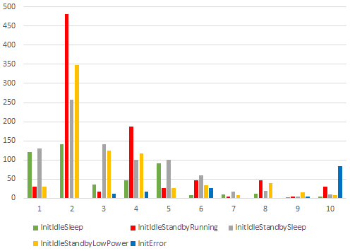 Figure 1
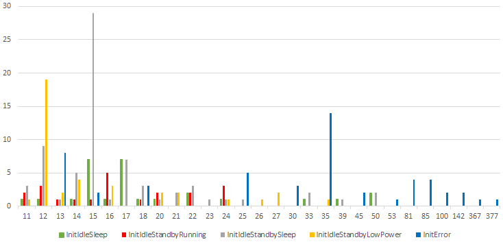 Figure 2
| Subalphabet | Number of states | Pairs of compatible states | Nodes in splitting graph | Depth distinguishing graph | Incompatible pairs not distinguished |
|---|---|---|---|---|---|
| InitIdleSleep | 1616 | 16638 (0.64%) | 1121 | 33 | 1145 (0.044%) |
| InitIdleStandbyRunning | 2855 | 14171 (0.17%) | 2082 | 33 | 2183 (0.027%) |
| InitIdleStandbySleep | 3168 | 25974 (0.26%) | 2226 | 33 | 3826 (0.038%) |
| InitIdleStandbyLowPower | 2614 | 13834 (0.20%) | 1809 | 33 | 2920 (0.043%) |
| InitError | 2649 | 373427 (5.3%) | 3097 | 35 | 17972 (0.27%) |
Peer Reviews
No public reviews on file for this paper yet. If you reviewed it on a platform where reviews are public (OpenReview, ICLR, NeurIPS, ICML), you can paste yours below so the community can read it here.
Videos
No videos yet. Explain this paper in a talk, walkthrough, or lecture? Add one.
Taxonomy
TopicsSoftware Testing and Debugging Techniques · Formal Methods in Verification · Web Application Security Vulnerabilities
11institutetext: Institute for Computing and Information Sciences,
Radboud University, Nijmegen, the Netherlands
petra, f.vaandrager@cs.ru.nl
State Identification for Labeled Transition Systems with Inputs and Outputs††thanks: Funded by the Netherlands Organisation of Scientific Research (NWO) under project 13859: Supersizing Model-Based testing (SUMBAT).
Petra van den Bos
Frits Vaandrager
Abstract
For Finite State Machines (FSMs) a rich testing theory has been developed to discover aspects of their behavior and ensure their correct functioning. Although this theory is widely used, e.g., to check conformance of protocol implementations, its applicability is limited by restrictions of the FSM framework: the fact that inputs and outputs alternate in an FSM, and outputs are fully determined by the previous input and state. Labeled Transition Systems with inputs and outputs (LTSs), as studied in ioco testing theory, provide a richer framework for testing component oriented systems, but lack the algorithms for test generation from FSM theory.
In this article, we propose an algorithm for the fundamental problem of state identification during testing of LTSs. Our algorithm is a direct generalization of the well-known algorithm for computing adaptive distinguishing sequences for FSMs proposed by Lee & Yannakakis. Our algorithm has to deal with so-called compatible states, states that cannot be distinguished in case of an adversarial system-under-test. Analogous to the result of Lee & Yannakakis, we prove that if an (adaptive) test exists that distinguishes all pairs of incompatible states of an LTS, our algorithm will find one. In practice, such adaptive tests typically do not exist. However, in experiments with an implementation of our algorithm on an industrial benchmark, we find that tests produced by our algorithm still distinguish more than 99% of the incompatible state pairs.
1 Introduction
Starting with Moore’s famous 1956 paper [16], a rich theory of testing finite-state machines (FSMs) has been developed to discover aspects of their behavior and ensure their correct functioning; see e.g. [12] for a survey. One of the classical testing problems is state identification: given some FSM, determine in which state it was initialized, by providing inputs and observing outputs.
Various forms of distinguishing sequences were proposed, ranging from sets of sequences to single sequences solving the problem. Moreover, when combined with state access sequences, so called -complete test suites can be constructed [8]. The challenge in using -complete test suites is to keep their size as small as possible. Using a single (adaptive) sequence for state identification [11], helps to reach this objective. If such a single sequence does not exist, then a distinguishing sequence distinguishing most states may be supplemented with some additional distinguishing sequences that distinguish the remaining states [15].
Although state identification algorithms for FSMs have been widely used, e.g., to check conformance of protocol implementations, their applicability is limited by the expressivity of the FSM framework. In FSMs, inputs and outputs strictly alternate, outputs are fully determined by the previous input and state, and inputs must be enabled in every state. Labeled Transition Systems with inputs and outputs (LTSs), as studied in ioco testing theory [24], provide a richer framework for testing component oriented systems: transitions are labeled by either an input or an output, allowing any combination of inputs and outputs, multiple outputs may be starting from the same state, allowing (observable) output nondeterminism, and states do not need to have transitions for all inputs, allowing partiality. However, LTSs lack the algorithms for test generation from FSM theory. Although progress has been made in defining and constructing -complete test suites for LTSs [4], an algorithm to solve the state identification problem as in [11], and hence to provide slim -complete test suites, is missing.
Therefore we generalize the construction algorithms for adaptive distinguishing sequences, as given in [11]. As in [4], we have to face the problem of compatible states [18, 20], which does not occur for FSMs. States are compatible when they cannot be distinguished in case of an adversarial system-under-test, e.g. when two states have a transition for the same output to the same state. As it is easy to construct LTSs with compatible states, we made sure our algorithms can deal with such LTSs: they accept LTSs with compatible states, but they ‘work around’ them, dealing with all incompatible states.
The outline of the paper is as follows. We first introduce graphs, LTSs, and some syntax for denoting trees. Then we elaborate on compatibility and the related concept of validity. Furthermore, we introduce test cases, and define when they distinguish states of an LTS. After that we define a data structure called splitting graph, present an algorithm that constructs a splitting graph for a given LTS, and another algorithm that extracts a test case from a splitting graph. We show that, unlike for FSMs, the splitting graph may have an exponential number of nodes. However, this is worst case behaviour, as our experiments on an industrial case study will show. Analogous to FSMs, it may not be possible to distinguish all states of an LTS with a single test case. Our experiments show that this is typically the case in practice, but nevertheless more than 99% of the incompatible state pairs are distinguished by the constructed test case. Following [11], we show that our algorithms constructs a test case distinguishing all incompatible state pairs, if it exists.
Related work
There are (at least) three ortogonal ways in which the classical FSM (or Mealy machine) model can be generalized.
A first generalization is to add nondeterminism. Whereas an FSM has exactly one outgoing transition for each state and input , a nonderministic FSM allows for more than one transition. Alur, Courcoubetis & Yannakakis [1] propose an algorithm to generate adaptive distinguishing sequences for nondeterministic FSMs, using (overlapping) subsets of states, similar to our algorithm. However, their sequences only distinguish pairs of states, and are not designed to distinguish more states at the same time. In between FSMs and nondeterministic FSMs we find the observable FSMs, which have at most one outgoing transition for each state , input and output ; one may use a determinization construction to convert any nondeterministic FSM into an observable one. The LTSs that we consider have observable nondeterminism.
A second generalization of FSMs is to relax the requirement that each input is enabled in each state. In a partial FSM, states do not necessarily have outgoing transitions for every state and every input. Petrenko & Yevtushenko [17] derive complete test suites for partial, observable FSMs, which is the closest to the automata model that we study in this paper. Their test generation is based on (adaptive) state counting [10], which is a trace search-based method which recognizes when states are distinguished, but does not provide a constructive way to build a test that distinguishes (many) states at once. Yannakakis & Lee [26] present a randomized algorithm which generates, with high probability, checking sequences, i.e., -complete test suites consisting of a single sequence. This approach is also applicable to partial FSMs, as opposed to the adaptive distinguishing sequence construction algorithms of [11], which apply to plain FSMs.
A third generalization of FSMs is to relax the requirement that inputs and outputs alternate. In our LTS, inputs and outputs may occur in arbitrary order. Bensalem, Krichen & Tripakis [19] give an algorithm for extracting adaptive distinguishing sequences for all states of a given LTS, by translating back and forth between a corresponding Mealy machine. This translation is only possible, if all states of the LTS have at most one outgoing output transition. Van den Bos, Janssen & Moerman [4] do not need such a restriction. They propose an algorithm that generates an adaptive distinguishing sequence for all pairs of incompatible states. In this paper, we generalize the result of [4] to distinguish more states at the same time.
2 Preliminaries
We write to denote that is a partial function from to . We write to mean , i.e., the result is defined, and if the result is undefined. We often identify a partial function with the set of pairs .
If is a set of symbols then denotes the set of all finite words over . The empty word is denoted by , the word consisting of symbol is denoted , and concatenation of words is denoted by juxtaposition.
Throughout this article, we use standard notations and terminology related to finite directed graphs (digraphs) and finite directed acyclic graphs (DAGs), as for instance defined in [6, 2]. If is a digraph and , then we let , or briefly , denote the set of direct successors of , that is, . Similarly, , or briefly , denotes the set of direct predecessors of , that is, . Vertex is called a root if , a leaf if , and internal if . We write , and .
The automata considered this paper are deterministic, finite labeled transition systems with transitions that are labeled by inputs or outputs. Since a single state may have outgoing transitions labeled with different outputs, and since outputs are not controllable, the behavior of our automata is nondeterministic: in general, for a given sequence of inputs, the resulting sequence of outputs is not uniquely determined. Nevertheless, our automata are deterministic in the sense of classical automata theory: for any observed sequence of inputs and outputs the resulting state is uniquely determined. We say that our automata have observable nondeterminism.
Because the inputs and outputs will be fixed throughout this article, we fix and as nonempty, disjoint, finite sets of input and output labels, respectively, and write . We will use to denote input labels, to denote output labels, and for labels that are either inputs or outputs.
Definition 1
An automaton (with inputs and outputs) is a triple with a finite set of states, a transition function, and the initial state. We associate a digraph to as follows
[TABLE]
Concepts and notations for extend to . Thus we say, for instance, that automaton is acyclic when is acyclic, and we write for the set of direct successors of a state . For and we write for , that is, the automaton obtained from by replacing the initial state by .
Figure 1 shows an example automaton. Below, we recall the definitions of some basic operations on (sets of) automata states. Operations , and retrieve all the inputs, outputs, or labels enabled in a state, respectively. To every set of states and every sequence of labels we can associate three sets of states: , , and . The set comprises all states that can be reached starting from a state of via a path with trace , whereas the set consists of all the states from where it is possible to reach a state in via a trace in , and consists of all states in from where a path with trace is possible. The traces operation provides the sequences of labels that can be observed from one or more of the states. We use a subscript if confusion may arise due to the use of several automata in the same context, e.g. denotes the enabled outputs of in automaton .
Definition 2
Let be an automaton, , and . Then we define:
[TABLE]
[TABLE]
Definitions are lifted to sets of states by pointwise extension. Thus, for , , , etc. We sometimes write the automaton, instead of the singleton set containing the initial state.
We find it convenient to use a fragment of Milner’s Calculus of Communicating Systems [14] as syntax for denoting acyclic automata. In particular, its recursive definition will allow us to incrementally construct test cases in Sections 5 and 6.
Definition 3
The set of expressions is defined by the BNF grammar
[TABLE]
The set is the smallest set of triples such that, for all and ,
2. 2.
If then 3. 3.
If then
An expression is deterministic iff, for all subexpressions of ,
[TABLE]
To each deterministic expression we associate an automaton , where is the set of subexpressions of , and transition function is defined by
[TABLE]
Example 1
The CCS expression has subexpressions , , , , and . These are the states of its associated automaton. The automaton’s transition relation is: . Note that states and are not reachable from initial state .
Suspension automata are automata with the additional property that in each state at least one output label is enabled. We note that this requirement can be easily enforced by adding a self-loop for an additional output label, that denotes ‘no-output’ or quiescence [24], in each state that has no output transition. We note that our definition of suspension automata, which is taken from [4], is more general than the one from [24, 25], since we only require states to be non-blocking, while suspension automata from [24, 25] adhere to some additional properties associated to this special quiescence output.
Definition 4
Let be an automaton. We call a state blocking if , and call non-blocking if none of its states is blocking. A non-blocking automaton is also called a suspension automaton.
We will use suspension automata as the specifications to derive test cases from. Figure 1 shows a suspension automaton. Plain automata are sometimes used as an intermediate structure to do computations, and test cases will be acyclic automata adhering to some additional properties.
3 Validity and Compatibility
In this section, we recall the definitions of the related notions of validity and compatibility [4]. We first give an efficient algorithm for computing valid states. After that, we show how the relation between validity and compatibility can be used to efficiently compute all pairs of compatible states occurring in a suspension automaton. We will need this last relation when constructing test cases to distinguish incompatible states.
3.1 Validity
We consider the following 2-player concurrent game, which is a minor variant of reachability games studied e.g., in [13, 5]. Two players, the tester and the System Under Test (SUT), play on a state space consisting of an automaton . At any point during the game there is a current state, which is initially. To advance the game, both the tester and the SUT choose an action from the current state :
- •
The tester chooses either an input from , or the special action . By choosing , the tester indicates that she performs no input and allows the SUT to execute any output he wishes.
- •
The SUT chooses an output from , or if no output is possible.
The game moves to a next state according to the following rule (this is the input-eager assumption from [5]): If the tester chooses an enabled input this will be executed, i.e., the current state changes to ; if the SUT chooses an enabled output this will only be executed when the tester has chosen , in this case the current state changes to ; when both players choose , the game terminates. The tester wins the game if she reaches a blocking state, and the SUT wins if he has a strategy that ensures that the tester will never win. A (memoryless) strategy for the tester is a function . We say a strategy is winning if the tester will always win the game (within a finite number of moves) when selecting actions according to this strategy, no matter which actions the SUT takes. Following Beneš et al [3] and Van den Bos et al [4], we call states for which the tester has a winning strategy invalid, and the remaining states in valid. The sets of valid and invalid states are characterized by the following lemma (cf Proposition 2.18 of [13]):
Lemma 1
Let be an automaton.
The set of invalid states of is the smallest set such that if
[TABLE] 2. 2.
The set of valid states of is the largest set such that implies
[TABLE]
Based on Lemma 1(1), Algorithm 1 computes the set of invalid states of an automaton and, for each invalid state , the first move of a winning strategy for the tester, as well as the maximum number of moves required to win the game.
Algorithm 1 is a minor variation of the classical algorithm for computing attractor sets and traps in 2-player concurrent games [13] and the procedure described by Beneš et al [3], which takes as input an automaton, of which each state has , and prunes away invalid states. Key invariants of the while-loop of lines 13-33 are that states in are invalid, and for , gives the number of output transitions to states in .
Let be the number of states in , and the number of transitions in . We assume, for convenience, that . If we use an adjacency-list representation of and represent the set of incoming transitions using a linked list, then the time complexity of the initialization part (lines 2-11) is . The while-loop (lines 13-33) visits each transition of at most twice (in lines 15 and 26) and performs a constant amount of work. Thus the time complexity of the while loop is . This means that the time complexity of Algorithm 1 is also .
The next lemma states some basic properties of the function that records the maximum number of moves required to win.
Lemma 2
Let be an automaton and the set of invalid states of . Let and be as computed by Algorithm 1. Then, for all and ,
* is blocking,* 2. 2.
, 3. 3.
.
3.2 Compatibility
Two states of a suspension automaton are compatible [18, 20] if a tester may not be able to distinguish them in the presence of an adversarial SUT. For example, if the tester wants to determine whether the SUT behaves according to state 2 or 3 of the suspension automaton of Figure 1, taking output transition will result in reaching state 4, from both states, but after reaching state 4, it cannot be determined, from which of the two states the transition was taken. Hence, states 2 and 3 are compatible.
Definition 5
Let be a suspension automaton. A relation is a compatibility relation if for all we have
[TABLE]
Two states are compatible, denoted , if there exists a compatibility relation relating and . Otherwise, the states are incompatible, denoted by . For a set of states, we write to denote that all states in are pairwise compatible, i.e., .
We note that the compatibility relation is symmetric and reflexive, but not transitive. For an elaborate discussion of compatibility, we refer the reader to [4]. The notions of compatibility and validity can be related using the following synchronous composition operator:
Definition 6
Let and be automata. The synchronous composition of and , notation , is the automaton , where transition function is given by:
[TABLE]
The next lemma asserts that states and are compatible precisely when the pair is a valid state of composed with itself.111This is a variation of Lemma 22 from [4], which is stated for a slightly different composition operator that involves demonic completions. Adding demonic completions is useful in the setting of [4], but not needed for our purposes.
Lemma 3
Let be a suspension automaton with . Then if and only if is a valid state of .
Proof
() Suppose that is a valid state of . Then, by Lemma 1(1), is contained in the largest subset of the states of that satisfies the conditions of Lemma 1(2). Using Definition 6, we infer that, for all :
[TABLE]
But this means that is a compatibility relation, and therefore .
() Suppose that . Then, by Definition 5, there exists a compatibility relation relating and . Since , is a subset of the set of states of . By combining Definitions 5 and 6, we infer that is the set from Lemma 1(2). This implies that is a valid state of . ∎
Example 2
Figure 2 shows the synchronization of the suspension automaton of Figure 1. It has 6 valid states, and in particular it shows that .
Lemma 3 suggests an efficient algorithm for computing compatibility of states. Suppose is a suspension automaton with states and transitions, with . Then we may compute composition in time . The idea is that we first sort the list of transitions on the value of their action label, which takes time. Next we check for each transition what are the possible transitions that may synchronize with . Since may only synchronize with -transitions, and since there are at most -transitions (as is deterministic), we may compute the list of transitions of the composition in time. Thus, the overall time complexity of computing is . The composition has states and transitions. Next we use Algorithm 1 to compute the set of invalid states of , which requires time. Two states and of are compatible iff is not in this set. Altogether, we need time to compute the compatible state pairs.
4 Test Cases
In this section, we introduce a simple notion of test cases. The goal of these test cases is state identification, i.e., to explore whether a state of the SUT, that is reached after some initial interactions, has the same traces as the state where it should be according to a given suspension automaton. Our test cases are adaptive in the sense that inputs that are sent to the SUT may depend on previous outputs generated by the SUT. They are similar to the adaptive distinguishing sequences of Lee & Yannakakis [11], except that inputs and outputs do not necessarily alternate, and the graph structure is a DAG rather than a tree.
Definition 7
A test case is an acyclic automaton such that each state enables either a single input action, or zero or more output actions. We refer to states that enable a single input as input states, and states that enable at least one output as output states. Thus each state from a test case is either an input state, an output state, or a leaf.
To each test case we associate a set of observations: maximal traces that we may observe during a run of .
Definition 8
For each test case , is the set of traces that reach a leaf of : .
Given a suspension automaton , we only want to consider test cases that are consistent with in the sense that each input that is provided by is also specified by , and conversely each output that is allowed by also occurs in .
Definition 9
Let be a test case and a suspension automaton. We say that is a test case for if, for each state of reachable from the initial state :
- •
if is an input state then ,
- •
if is an output state then .
We say is a test case for state if is a test case for . Furthermore, is a test case for a set of states if is a test case for all .
Lemma 4
Suppose is a test case for a set of states of suspension automaton . Suppose that , for some label and state . Then is a test case for .
If is a test case for a suspension automaton then the composition is also a test case. We can view as the subautomaton of in which all outputs that are not enabled in have been pruned away. A test case distinguishes two states, if the states enable different observable traces of the test case.
Lemma 5
If is a test case for a suspension automaton , then the composition is also a test case for , satisfying .
Definition 10
Let be a test case for states and of suspension automaton . Then distinguishes and if .
Example 3
The associated automaton of the CCS expression (see Example 1) is a test case for states 1 and 2 of the suspension automaton from Figure 1. Its observable traces are , and it distinguishes states 1 and 2.
Lemma 6
Let be a suspension automaton with . Then iff there exists a test case that distinguishes and .
Proof
By Lemma 3, iff the pair is an invalid state of . By definition, this means that in the game for the tester has a winning strategy . This strategy can be effectively computed by Algorithm 1. Using strategy , we compute a test case as follows:
- •
The set of states consists of the set of invalid states of , extended with a single leaf state .
- •
The initial state is .
- •
The transition relation of is obtained by (a) restricting the transition relation of to , (b) removing all input transitions, except the outgoing transitions with label from states with , (c) adding an output transition for each and such that and does not have an outgoing -transition.
It is routine to check that is a test case for states and of . We claim that distinguishes and , that is, . Because suppose . Then corresponds to a run from initial state of to leaf node . By construction of , must be of the form , where corresponds to a run in from to some state and . This means that has a run with actions from initial state to state . However, since , . By a symmetric argument, we may conclude that implies . Thus , as required. ∎
The following definition generalizes the notion of adaptive distinguishing sequence for FSM’s [9, 11] to the setting of suspension automata.
Definition 11
Let be a suspension automaton, , and a test case for . We say that is an adaptive distinguishing graph for if, for all with , distinguishes and . Test case is an adaptive distinguishing graph for if it is an adaptive distinguishing graph for the set of states of .
Just like there are FSMs without an adaptive distinguishing sequence, there are suspension automata for which no adaptive distinguishing graph exists. This is the case for the suspension automaton from Figure 3. We cannot construct an adaptive distinguishing graph by choosing the root node to be an output state, since states 1 and 3 cannot be distinguished, as they both go to state 2 with their single output transition . The root also cannot be an input state for either of all inputs or . After , states 1 and 2 both reach state 1, and after , states 2 and 3 both reach state 3.
In the remainder of this paper, we present algorithms for constructing an adaptive distinguishing graph for from a suspension automaton , if it exists.
5 Splitting Graphs
In this section, we present the concept of a splitting graph, as well as an algorithm for constructing such a graph. Our algorithm generalizes the algorithm of Lee & Yannakakis [11] for computing a splitting tree for an FSM. In the next section, we will construct an adaptive distinguishing graph by extracting its parts from the splitting graph. An adaptive distinguishing graph that distinguishes all incompatible state pairs, is only guaranteed to be found, if some additional requirements on the splitting graph construction are satisfied. We will delay the discussion of adaptive distinguishing graphs to the next section, and focus on splitting graphs first.
We will first give the definition of a splitting graph, and the outer loop of our algorithm for constructing it. Then we define when a leaf node of a splitting graph is splittable (i.e., when child nodes can be added), and show that a splittable leaf exists whenever some leaf contains incompatible states. After that, we explain how to construct the child nodes for splittable leaves.
5.1 Splitting Graph Definition
A splitting graph for suspension automaton is a directed graph in which the vertices are subsets of states of ; there is a single root , and an internal node is the union of its children. We require that, for each edge of the splitting graph, is a proper subset of ; this implies that a splitting graph is a DAG. We associate a test case to each internal node and require a tight link between the observations of and the children of : each observation has one child that contains all states enabling . As we have , this means that, after following any trace from test case , the states have been distinguished from states from the states .
Definition 12
A splitting graph for suspension automaton is a triple with
- •
- •
such that
is the only root of , 2. 2.
, and 3. 3.
.
- •
is a witness function such that, for all internal vertices , is a test case such that:
.
Splitting graph is complete if, for each leaf , the states contained in are pairwise compatible, i.e., .
Algorithm 2 shows the main loop for constructing a splitting graph for a given suspension automaton. The idea is to start with the trivial splitting graph with just a single node, and then repeatedly split leaf nodes, i.e., add child nodes, until all leaves only contain pairwise compatible states. This means that incompatible states are in different leaves when the algorithm terminates. Since nodes in a splitting graph are finite sets of states, and children are strict subsets of their parents, Algorithm 2 terminates after a finite number of refinements. With , we denote the empty function.
5.2 Splitting Conditions
Before we elaborate on the algorithm for the method splitnode, we first explore what conditions should hold for a leaf to be splittable. The formal definition of these conditions is given below in Definition 14.
If we are lucky we can find, for each output , a state that does not enable . In this case, observing an output allows us to distinguish at least one state from some other states. Otherwise, we may check whether, for certain enabled inputs, or all outputs, the states of have a transition to the states of an internal node, i.e., a node that has already been split, because then may be split as well when these labels occur. In particular, the states of can be split for some label if the reached node is a least common ancestor of . An internal node is least common ancestor for a set of states if it contains but none of its children does.
Definition 13
Let be a splitting graph for suspension automaton and let be a set of states of . An internal node of is a least common ancestor of if and, for all , . We write for the set of least common ancestors of contained in .
Note that we can compute the set of least common ancestors for any set in a time that is linear in the size of the splitting graph.
Definition 14
Let be a splitting graph for suspension automaton .
A leaf of is splittable on output if
[TABLE] 2. 2.
A leaf of is splittable on input if
[TABLE]
A leaf of is splittable if it is splittable on output or splittable on input.
Lemma 7
Each incomplete splitting graph has a splittable leaf.
Proof
Let be an incomplete splitting graph for suspension automaton . Since is incomplete, there is at least one leaf that contains a pair of incompatible states. By Lemma 3, we have that for all states of , iff is an invalid state of . Using Algorithm 1, we may therefore compute the pairs of incompatible states of and functions and on these pairs. Let be the leaf node that contains a pair of incompatible states for which the value is minimal. We claim that is a splittable leaf of . There are three cases:
Suppose . Then, by Lemma 2(1), is a blocking state of . This implies that . But this means that, for each output action , either or . Therefore, can be split on output. 2. 2.
Suppose and . Then, by Lemma 3 and Lemma 2(2), both and enable input and, writing and , we have , , and . Since none of the leaves contains a pair of incompatible states with a value smaller than , we know that does not have a leaf node that contains both and . But this implies that , and so can be split on input. 3. 3.
Suppose and . Let . If there exists an such that then we may split on output. Otherwise, both and enable output . Write and . Then and . By Lemma 3 and Lemma 2(2), . Since none of the leaves contains a pair of incompatible states with a value smaller than , we know that does not have a leaf node containing both and . But this implies that , so can be split on output. ∎
5.3 Splitting Graph Construction
Based on the condition of Definition 14 that holds, we assign children to splittable leaf nodes, and update the witness function. This is worked out in the method splitnode of Algorithm 3. The algorithm may choose nondeterministically between a split on output or a split on input, if both are possible. Such a choice is denoted with the syntax for guarded commands [7], i.e., as the guards on lines 5 and 16, and their respective statements on lines 6-15, and 17-20.
If a leaf is split on output, then children are added for each output . If , then we add as a child, as those are the only states from which can be observed. We also add (i.e., by using +) the term to the witness of , as observing distinguishes states in from states in .
If , observing will not distinguish any states. We then use that there is a , which means that some states of are distinguished by the witness . Hence, by taking output , followed by , some states of are distinguished. Therefore, we add to the witness of , and split in the same way was split, i.e., if are all the states with for some child , then is a child of . We call such a split an induced split.
For splitting on some input , we also use an induced split to obtain the children for . Since there exists some , at least two states of may be distinguished by the witness constructed for , after taking input . To each element of the induced split, we add all the states not enabling . If we would not do this, Algorithm 3 may assign the empty set as children to a splittable leaf, such that it remains a leaf. As a consequence, Lemma 8 and also Corollary 1 then do not hold. This will be illustrated by Example 5. Corollary 1 shows termination of our splitting graph construction algorithm. It follows from the consecutive application of Lemma 8.
Definition 15
Let be a splitting graph for suspension automaton . Let be an internal node of , a set of states of , and , such that . Then the induced split of with to is:
[TABLE]
Example 4
We compute the splitting graph of the suspension automaton from Figure 1, using Algorithm 2, and show the result in Figure 4(left).
For the root node , we observe that state 4 does not enable , while states 2 and 3 do not enable . Hence, the root is split on output, gets children and , and witness .
Node can be split on input , as states 1 and 2 enable , and since the root node is an LCA of : from and , we obtain that the root node is an LCA, since , but , and . The induced split is . We then need to add state 3 to both sets, because state 3 does not enable , so node {1,2,3} gets children {1,3} and {2,3}. Prepending to the witness of the root node gives us witness for .
Node can be split on output. As state 4 does not enable , we only need to find an LCA for , which is the previously split node . For we have witness , and for we use the witness of , so the witness for {1,4} is .
Next, node {1,3} can be split on output using {1,4} as LCA for . Node {2,3} does not need to be split, as we have . All other leaves are singletons, so we have obtained a complete splitting graph.
Example 5
Figure 5 shows that using only the induced split as children, for splitting a leaf on input, results in an incomplete splitting graph. The construction of the splitting graph goes as follows. The root node {1,2,3,4,5} can be split on output, as each state only enables one of the three outputs , , and : we obtain children {{1,2,7},{8},{3,4,5,6}}. Leaf {1,2,7} can be split on output, as shows that we can use the root node as LCA. Leaf {3,4,5,6} cannot be split on output as , so there exists no LCA for . It can be split on input : , so we can use the root node as LCA. Then , so these are added as children. It remains to split {1,2}, as they are incompatible: a test case with observations distinguishes 1 and 2. Leaf {1,2} cannot be split on input, as , so no LCA exists. For input we find that = {3,4}, and {3,4,5,6} is an LCA. However, , as both 3 and 4 are not contained in any child of {3,4,5,6}. Hence, we obtain , which means by definition that {1,2} is a leaf. Algorithm 2 will keep trying to split {1,2} indefinitely, and will hence not terminate.
Lemma 8
Algorithm 3 returns a splitting graph for , when given some splitting graph , such that one leaf of , has become an internal node in .
Proof
The input of Algorithm 3 is a splitting graph for . All the algorithm does is to take a single leaf node , add children to it, and extend the evaluation function for some witness to . This means that it in order to prove that Algorithm 3 returns a splitting graph, it suffices to show that (a) for all , , (b) , (c) is a test case, and (d) , and (e) .
To prove (a) we inspect the three places in the algorithm where a new element was added to the set of children of : line 8, line 12 and line 18:
- •
Line 8: In this case and there exists a such that output is not enabled from state . This implies , as required.
- •
Line 12: In this case, let for some . By definition of , and there is a such that . Note that this implies . By definition of LCA, there exists a with . Because , there exists a state such that . Since , we know that . Hence , as required.
- •
Line 18: In this case, , where and . By definition of , and there is a such that . This implies . By definition of LCA, there exist such that . Because , there exists a state such that . Since , we know that . This means and thus . Hence , as required.
For proving (b), it remains to show that . Choose . We consider two cases:
- •
A split on output was performed (line 5-15). Since is a suspension automaton, there is at least one output that is enabled in . If there is another state in that does not enable then is added to and thus , as required. Otherwise, sets are added to , for and some . Let . Since and , there is some with . This implies and therefore , as required.
- •
A split on input was performed (lines 16-20). In this case, the sets are added to , for , some input and . If state does not enable input then state is in each set that is added to , and thus , as required. Now suppose enables input . Let . Then and thus . Since , there is some with . Therefore, , and therefore , as required.
For proving (c) we again consider the two cases of splitting on output or input:
- •
If a split on output was performed, then root of is an output state, as each observation has an output prefix: on line 9 or 13 either or for some are added to . Since is a test case, and is a test case since is an internal node of , is also a test case.
- •
If a split on input was performed, then the root of is an input state, as it enables a single input according to line 20: for some . As is a test case since is an internal node of , is also a test case.
For proving (d), we inspect the three places in the algorithm where children were added to , and where witness observations were added to . We will show that for each added observation , a child constructed at the same place can be used to prove .
- •
On lines 8 and 9, a child was added to , and observation was added to . Hence, for we have child with .
- •
On lines 12 and 13, children are added to , and observations are added to for all , using some . Since is an internal node of , there is a such that . If , then it holds that , so from (by ) it then follows that . Hence any can be used to show as . Else, there is some with . Let , and observe that . From and it then follows that , so . It follows that .
- •
On lines 19 and 20 children for all are assigned to , and observations are added to for all , using some . Again, since is an internal node of , there is a such that . If , then it follows, with similar arguments as for lines 12 and 13, that . Since , and hence also , we can use any child from line 12 to show . Else, there is some with . With the same reasoning as for lines 12 and 13, we obtain . By again using that , we obtain .
For proving (e) we consider the two cases of splitting on output or input:
- •
Suppose an output split is performed. The body of the for-loop on lines 7-14 is then executed at least once, since the algorithm only accepts suspension automata, so each state is non-blocking, and consequently . Hence, suppose that the for-loop is executed for some . To prove that , we now need to show that (line 8), and that (line 12), using some (line 11).
For line 8, we use from (a) that , so .
For line 12, we need to prove that there exists a such that . Because there is some , we have . Since , there is a , so . Because , there is a with . Hence, . It then follows that .
- •
Suppose an input split is performed for some input . We then have a with , for the same reasons as given for line 12. Consequently, . Adding the (possibly empty) set to each element of results in a non-empty set . ∎
Corollary 1
Algorithm 2 returns a complete splitting graph for .
The algorithm of [11] constructs a splitting tree in polynomial time, because leaves of a node form a partition of that node. Our splitting graphs do not have this property. Clearly, a splitting graph for a suspension automaton with states cannot have more than nodes, as the set of nodes is a subset of by Definition 12. For with , consider suspension automaton , where consists of the following output transitions:
[TABLE]
Figure 6 depicts suspension automata for . We can prove Lemma 9 by showing that has a splitting graph with nodes.
Lemma 9
Let be a suspension automaton with states. Then a splitting graph returned by Algorithm 2 has nodes. This bound is tight.
Proof
We already showed that a splitting graph has at most an exponential number of states. We will now prove that Algorithm 2 returns a splitting graph with exactly nodes for suspension automaton with :
We first note that different states are pairwise incompatible, since we can easily construct a test case identifying any of the states: observing output , after having observed (other) outputs, means that the test case was executed from state . Consequently, if a node of the split graph contains more than 1 state, it has children.
The root node is split on output, so it has children for all size subsets of , and it has child . We now show that the split graph has nodes for all non-empty subsets of , except trivial subset .
Suppose we have a non-trivial subset of with at least two elements. For all state does not enable output , but all other states of do, so we obtain child by a split on output . By repeatedly removing a single element by splitting on that element, we can show that the split graph contains a node for any nonempty, non-trivial subset of . There are nonempty, non-trivial subsets of . In addition, the split graph also has nodes and . Hence, in total the splitting graph has nodes. ∎
6 Extracting Test Cases from a Splitting Graph
Algorithm 4 retrieves CCS terms, of which the associated automata are test cases that distinguish states. The algorithm “concatenates” several CCS terms while keeping track of the current set of states. Each CCS term ensures that one state is distinguished from the rest because it lacks some output. We compute the current states for the leaves of the CCS term, and attach another CCS term to this leaf, if the current set of states consists of some incompatible pair of states. Hence in total, the automaton of the resulting CCS term distinguishes multiple pairs of states.
Example 6
We construct the adaptive distinguishing graph for the suspension automaton from Figure 1, using the splitting graph from Figure 4, which also shows the result of this example. Algorithm 4 starts with and . Hence, we search for a least common ancestor for . This will be the root node of the splitting graph, with witness .
The function is then called with , and will result in two recursive calls of the function on line 13 for and , and and respectively. In the first case, the condition of line 10 holds, and we the function is called for and , which means that lines 8-9 are executed next, using the only LCA for {1,4}, namely {1,4}.
The algorithm will then do some more recursive calls, checking whether the witness of {1,4} must be extended further to distinguish more states. This will not be the case, because only singleton sets are reached at the leaves of the witness, and holds for any state , since is reflexive. Hence, we need to prepend to the witness of {1,4} to obtain the left term of the + operator of the resulting CCS term of the algorithm: .
As , its LCA {1,2,3} will be used to complete the construction of the right term of the + operator of the result.
The associated automaton of the resulting CCS term is an adaptive distinguishing graph for the suspension automaton, as it distinguishes all incompatible state pairs.
Lemma 10
Algorithm 4 terminates and outputs a CCS term that denotes a test case satisfying, for each , .
Proof
Let be the suspension automaton, and the splitting graph for , that we provide to Algorithm 4. We note that all computations are atomic, or reducing the size of the CCS expression before making a recursive call, except line 8. However, LCAs can be computed straightforwardly: start at the root, if it is not an LCA, continue with the children containing the set of states the LCA is computed for, and repeat. This procedure always succeeds in finign an LCA, due to the following argument. Any set of states, with at least two incompatible states, has a least common ancestor in the splitting graph, as the leaves of are sets of mutually compatible states, its root node contains all the states from , and all the states of a non-leaf are contained in at least one of its children, by Definition 12.
By construction, Algorithm 4 follows the labels of each for nodes obtained on line 8. By the property from Definition 12 that , and , we see that , so after visiting line 8 at most times, set will only contain mutually compatible states. ∎
Algorithm 4 does not always construct an adaptive distinguishing graph for all incompatible state pairs. To ensure this, it must be able to select an “injective” splitting node as LCA on line 8. This will guarantee that a transition never maps two incompatible states to two compatible states (which cannot be distinguished any more), or that an input is used that is not enabled in some states.
Definition 16
Let be a suspension automaton, a set of states, and a label. Then is injective for if
[TABLE]
Analogous to the result of [11], Theorem 6.1 asserts that if an adaptive distinguishing graph exists our algorithms will find it, provided there are no compatible states. This last assumption is motivated in Example 7. We first need to establish the following lemma.
Lemma 11
Let be a suspension automaton such that all pairs of distinct states are incompatible. Suppose is an adaptive distinguishing graph for a set of states of . Suppose that , for some label and state . Then is injective for and is an adaptive distinguishing graph for .
Theorem 6.1
Let be a suspension automaton such that all pairs of distinct states are incompatible. Then has an adaptive distinguishing graph if and only if, during construction of a splitting graph for , Algorithm 3 can and does only perform injective splits, that is, whenever Algorithm 3 splits a leaf on output, then is injective for , for all , and whenever it splits a leaf on input , then is injective for . Moreover, in this case Algorithm 4 constructs an adaptive distinguishing graph for , when is given as input.
Proof
Let .
() Suppose splitting graph for has been constructed using injective splits only. Then, for each internal node of , is a test case for : inputs performed by the test case will be enabled in all the corresponding states of . This means that also the CCS term computed from by Algorithm 4 will correspond to a test case for the set of states of . Since all the splits in are injective, we have that for any pair of incompatible states of , and for any observation of that is enabled in both and , the unique state in is incompatible with the unique state in . But since, by construction, only contains mutually compatible states, for each observation of , we conclude that distinguishes and . Therefore, is an adapaptive distinguishing graph for .
() Suppose is an adaptive distinguishing graph for .
Let be an incomplete splitting graph. We show that has a leaf for which an injective split exists.
Assume w.l.o.g. that is a tree (any DAG can be unfolded into a tree). We associate to each node of a height, which is the length of the maximal path from to a leaf. Also, we associate to each node of a set of states from called the current set: the current set of is , and if the current set of state is and then the current set of is . Lemma 11 implies that if the current set of equals , is an adaptive distinguishing graph for .
Now, amongst the leaves of that contains a maximal number of states, choose a leaf that is contained in the current set of a node of with minimal height. We consider two cases:
- •
is an input state of . Then enables a single input action . Let . Then the current set of is and the height of is less than the height of . By Lemma 11, is injective for . By definition of injectivity, is also injective for subset of . Since all pairs of distinct states of are incompatible, the number of states in equals the number of elements of . Moreover, since is contained in , and amongst the leaves of that contains a maximal number of states is contained in the current set of a node with minimal height, is not contained in any leaf of . Thus leaf is splittable on input , and this split is injective.
- •
is an output state of . Suppose . Then either there is a such that , or the number of states in equals the number of elements of and is not contained in any leaf of . This means that is splittable on output, with a split that is injective for each output . ∎
Example 7
Without the assumption that there are no compatible state pairs, Theorem 6.1 does not hold. The suspension automaton of Figure 7 has an adaptive distinguishing graph, but our algorithm does not find it. Note that states and are compatible, and also states and are compatible. An adaptive distinguishing graph for is denoted by CCS term . When we construct a splitting graph for , the set of all states will be split on output, resulting in children , , and . Now a split of on input is not injective and a split on input is not possible since the set of LCAs is empty. Similarly, there is no injective split of .
7 Experimental Results on a Case Study
In [22], an FSM model, with over 10.000 states, was learned of an industrial piece of software, called the Engine Status Manager (ESM). During the learning process, testing against the ESM posed a significant challenge: it turned out to be extremely difficult to find counterexamples for hypothesis models. Initially, existing conformance testing algorithms were used to find counterexamples for hypothesis models (random walk, W-method, Wp-method, etc), but for larger hypothesis models these methods were unsuccessful. However, adaptive distinguishing sequences as in [11], augmented with additional pairwise distinguishing sequences for states not distinguished by the adaptive sequence, were able to find the required counterexamples. Therefore, the ESM models are good candidates to show the strength of the adaptive distinguishing graphs of this paper too.
Of course, applying our adaptive distinguishing graphs directly on the Mealy machine models, would not show our capability to handle the more expressive suspension automata. We therefore transformed the FSM models in such a way that they exhibit output nondeterminism. We first split all Mealy transitions in two consecutive transitions and , and added a self-loop output transition ‘quiescence’ (denoting absense of response) to all states only having input transitions, to make it non-blocking. To ensure determinism, information about data parameters from the ESM was added to the labels of the Mealy machine in [22]. For our experiments, we removed this information again, resulting in suspension automata with states with multiple outgoing output transitions.
For performance reasons, we reduced the Mealy machine model with a subalphabet, before applying the transformation steps described above, i.e., we removed all transitions with not in the subalphabet. We obtained these subalphabets from [21], which contains a figure displaying interesting subalphabets based on domain knowledge. Table 1 shows that the resulting suspension automata still have a significant size.
We applied the algorithms of this paper to obtain a splitting graph and an adaptive distinguishing graph. The splitting graph was constructed as in Algorithm 3, so without requiring injectivity of the used labels. However, in the construction of the adaptive distinguishing graph (Algorithm 4) we chose on line 8 an LCA which was injective for the most pairs of states.
Table 1 shows that there are many pairs of incompatible states to distinguish. However, the number of nodes of the splitting graph are in the order of magnitude of the number of states of the suspension automaton, and the longest observable trace (i.e., the depth) of the adaptive distinguishing graphs is not long at all. Moreover, over 99% of the pairs of incompatible states are distinguished by the adaptive distinguishing graph. This indicates that the adaptive distinguishing graphs, although constructed from a non-injective splitting graph, can be very effective in testing.
To further explore the structure of the adaptive distinguishing graph, we computed the size of each leaf: the number of automaton states, that enable the observable trace to that leaf. We note that this includes states compatible to some of the automaton states. Additionally, states may enable multiple observable traces, and hence a single state may increase the size of several leaves. Figure 8 shows the results: the x-axis displays all leaf sizes, and a column of some subalphabet shows the number of leaves of this size (y-axis). We see that the majority of leaves are of small size, while leaves of larger size occur less. We see that subalphabet InitError has the most large leaves, which could explain the adaptive distinguishing graph’s relatively large number of pairs of incompatible states not distinguished.
8 Conclusions and Future Work
We studied the state identification problem for suspension automata, generalizing results from [11]. We presented algorithms to construct test cases that distinguish all incompatible state pairs, if possible, or many, if not. Experiments suggest that this approach is quite effective.
We see several directions for future research. First, though we did apply our algorithms to instances of an industrial benchmark, we would like to apply it to different case studies as well, to further explore the applicability of our approach. We note however that there are not that many (large) LTS benchmarks available.
An open problem is to give a bound on the depth of the distinguishing graph that our algorithms constructs. For FSMs, a quadratic bound is known [11], with examples to show it is tight [23, 11]. These examples extend to our setting, as we generalize from the FSM setting, but the proof for the quadratic bound on adaptive distinguishing sequences from [11] does not.
If our algorithm returns an adaptive distinguishing graph that does not distinguish all incompatible state pairs, the question remains how to efficiently distinguish these remaining states. Graphs distinguishing pairs of states can be obtained directly from our splitting graph, or by computing them as in [4], but distinguishing all remaining pairs results in a large overhead compared to the small size of the distinguishing graph we obtained in our experiments. On the one hand, we can optimize the obtained distinguishing graph by improving the splitting graph’s quality by applying heuristics that optimize the choice of labels for splitting leaves. On the other hand, we can use causes for states not being distinguished to construct a distinguishing graph that distinguishes all or at least many of the not distinguished states.
Though our distinguishing graphs significantly improve the size of an -complete test suite, the problem to compute good access sequences for such a test suite requires further research as well [4]. Due to the output nondeterminism of suspension automata, we need an input-fairness assumption, to ensure that all outputs enabled from a state may eventually be observed. However, for access sequences we rather have a more adaptive strategy, in the spirit of [5], that reacts on the outputs as produced by the tested system rightaway. Adaptively choosing access sequences means that for reaching the same state, different access sequences may be used. However, the proof of -completeness of a test suite depends on using one unique access sequence for accessing the same state. It remains an open problem whether using different access sequences breaks -completeness or not.
The reference list from the paper itself. Each links out to its DOI / PubMed record.
- 1[1] Rajeev Alur, Costas Courcoubetis, and Mihalis Yannakakis. Distinguishing tests for nondeterministic and probabilistic machines. In STOC , volume 95, pages 363–372. Citeseer, 1995.
- 2[2] Christel Baier and Joost-Pieter Katoen. Principles of Model Checking . The MIT Press, 2008.
- 3[3] Nikola Beneš, Przemysław Daca, Thomas A. Henzinger, Jan Křetínskỳ, and Dejan Ničković. Complete Composition Operators for IOCO-Testing Theory. In Proceedings of the 18th International ACM SIGSOFT Symposium on Component-Based Software Engineering , CBSE ’15, pages 101–110, New York, NY, USA, 2015. ACM.
- 4[4] Petra van den Bos, Ramon Janssen, and Joshua Moerman. n-Complete Test Suites for IOCO. Software Quality Journal , 27(2):563–588, Jun 2019.
- 5[5] Petra van den Bos and Marielle Stoelinga. Tester versus Bug: A Generic Framework for Model-Based Testing via Games. In Andrea Orlandini and Martin Zimmermann, editors, Proceedings Ninth International Symposium on Games, Automata, Logics, and Formal Verification, Saarbrücken, Germany, 26-28th September 2018, volume 277 of Electronic Proceedings in Theoretical Computer Science , pages 118–132. Open Publishing Association, 2018.
- 6[6] Thomas H. Cormen, Charles E. Leiserson, Ronald L. Rivest, and Clifford Stein. Introduction to Algorithms, Third Edition . The MIT Press, 3rd edition, 2009.
- 7[7] Edsger W. Dijkstra. Guarded commands, nondeterminacy, and formal derivation of programs. In David Gries, editor, Programming Methodology: A Collection of Articles by Members of IFIP WG 2.3 , pages 166–175, New York, NY, 1978. Springer New York.
- 8[8] Rita Dorofeeva, Khaled El-Fakih, Stephane Maag, Ana R. Cavalli, and Nina Yevtushenko. FSM-based conformance testing methods: A survey annotated with experimental evaluation. Information and Software Technology , 52(12):1286–1297, 2010.