Dynamic Input for Deep Reinforcement Learning in Autonomous Driving
Maria H\"ugle, Gabriel Kalweit, Branka Mirchevska, Moritz Werling,, Joschka Boedecker

TL;DR
This paper explores how Deep Sets can improve deep reinforcement learning for autonomous driving by effectively handling variable numbers of surrounding objects, leading to better performance and generalization.
Contribution
It demonstrates that Deep Sets outperform traditional neural network architectures in processing variable-sized inputs in reinforcement learning for autonomous driving.
Findings
Deep Sets achieve superior overall performance.
Deep Sets generalize better to unseen scenarios.
Traditional architectures face limitations with variable input sizes.
Abstract
In many real-world decision making problems, reaching an optimal decision requires taking into account a variable number of objects around the agent. Autonomous driving is a domain in which this is especially relevant, since the number of cars surrounding the agent varies considerably over time and affects the optimal action to be taken. Classical methods that process object lists can deal with this requirement. However, to take advantage of recent high-performing methods based on deep reinforcement learning in modular pipelines, special architectures are necessary. For these, a number of options exist, but a thorough comparison of the different possibilities is missing. In this paper, we elaborate limitations of fully-connected neural networks and other established approaches like convolutional and recurrent neural networks in the context of reinforcement learning problems that have to…
Click any figure to enlarge with its caption.
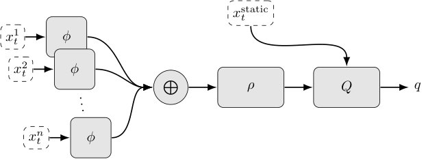 Figure 1
 Figure 2
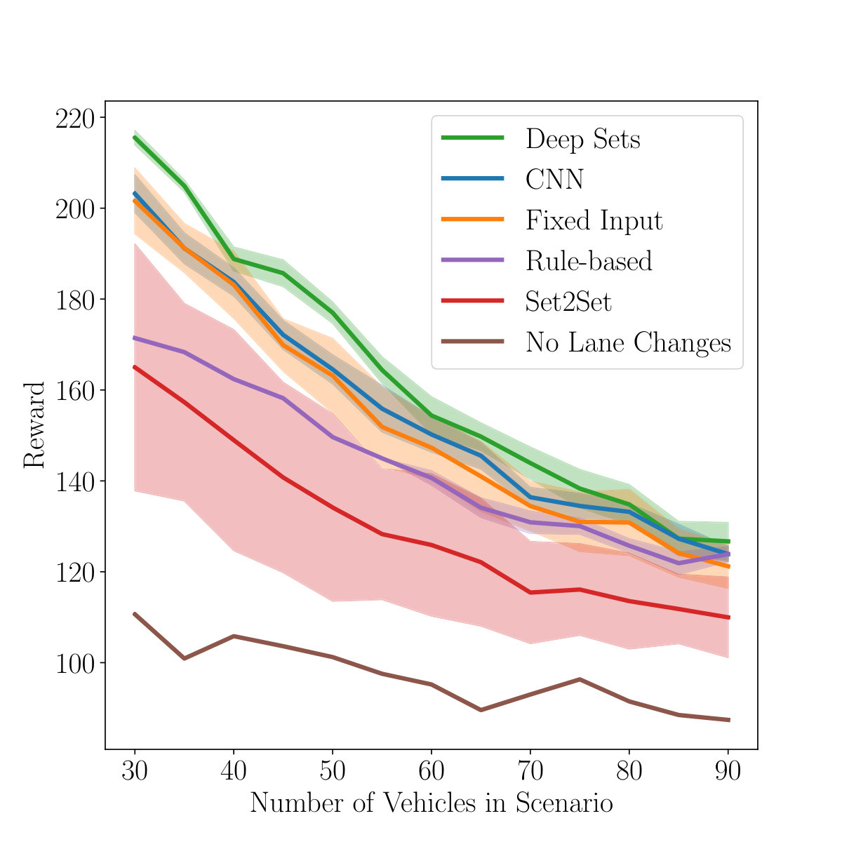 Figure 3
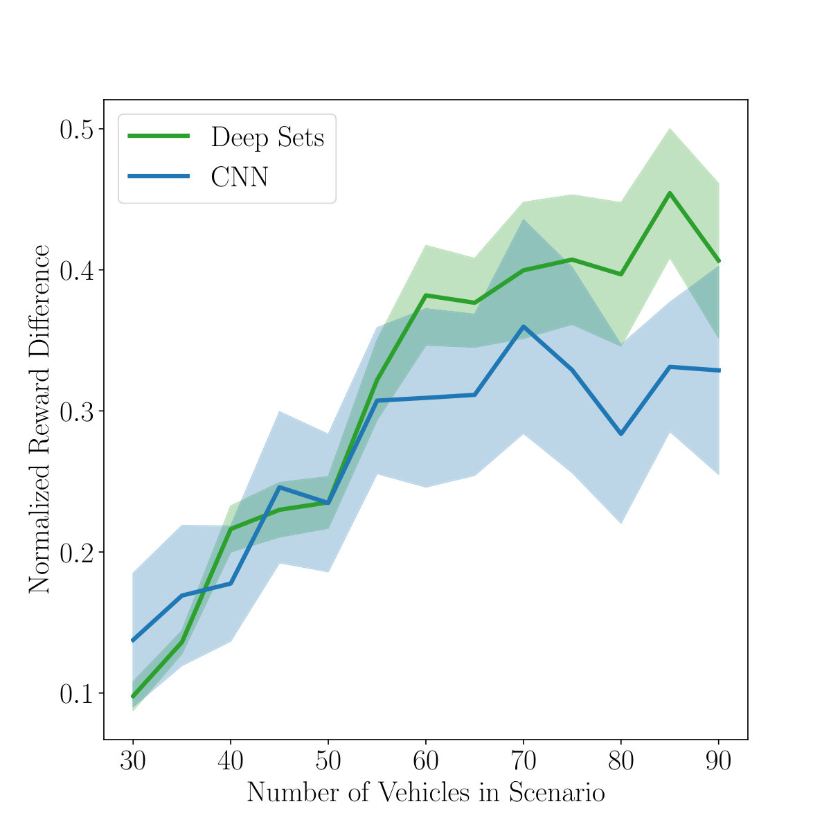 Figure 4
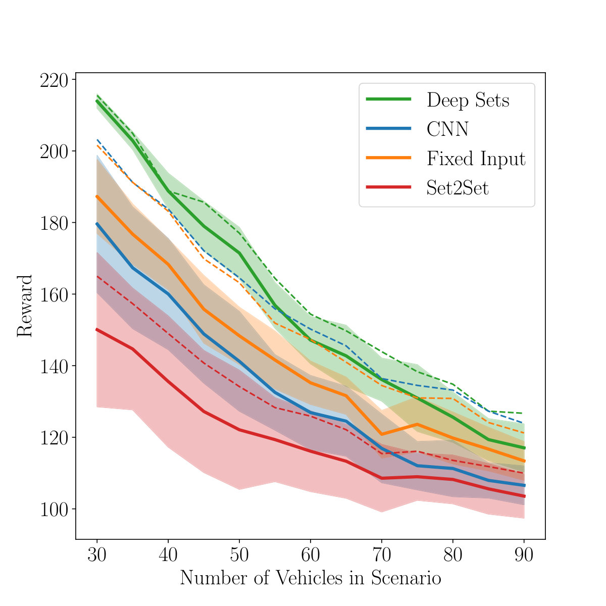 Figure 5
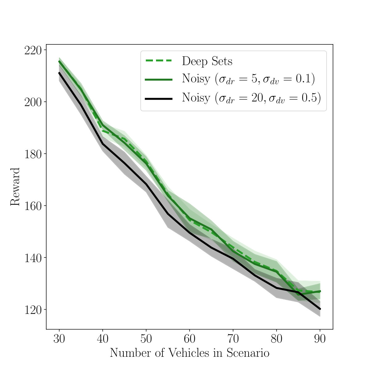 Figure 6
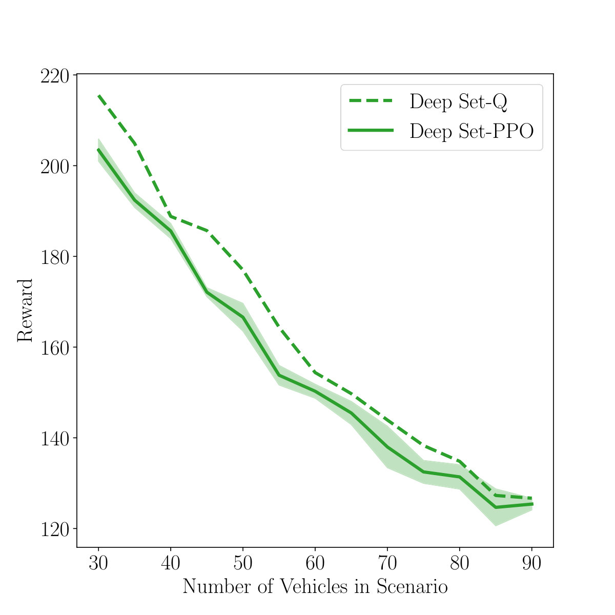 Figure 7
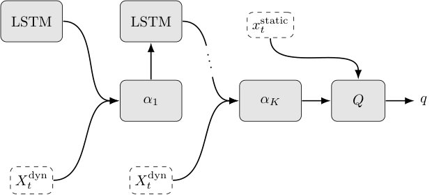 Figure 8
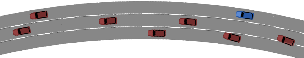 Figure 9
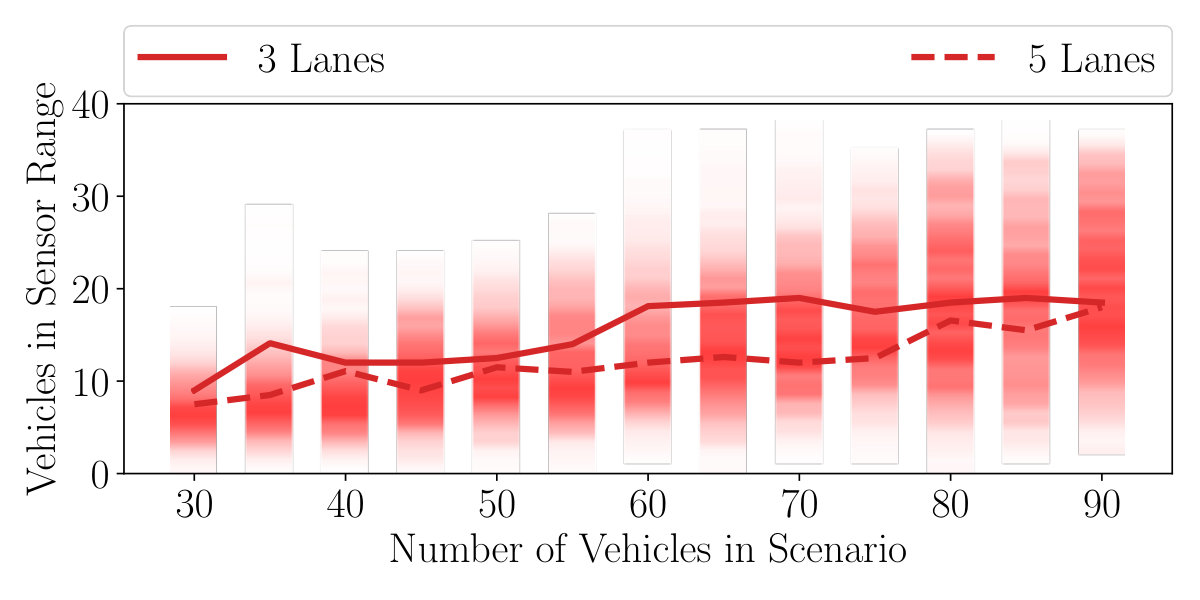 Figure 10
| Scenario | 30 | 50 | 70 | 90 |
|---|---|---|---|---|
| Fixed Input | 201.59 ( 7.23) | 163.17 ( 8.17) | 134.47 ( 5.45) | 121.21 ( 4.83) |
| CNN | 203.2 ( 4.15) | 164.54 ( 3.2) | 136.41 ( 2.15) | 123.9 ( 1.7) |
| Set2Set | 164.99 ( 27.17) | 134.15 ( 20.61) | 115.43 ( 11.22) | 109.98 ( 8.85) |
| Deep Sets | 215.51 ( 1.58) | 177.01 ( 2.35) | 143.93 ( 3.52) | 126.7 ( 4.14) |
| Scenario | 30 | 50 | 70 | 90 |
|---|---|---|---|---|
| Fixed Input | 187.26 ( 10.33) | 148.33 ( 8.0) | 120.83 ( 6.64) | 113.4 ( 5.4) |
| Set2Set | 150.06 ( 21.55) | 122.09 ( 16.64) | 108.56 ( 9.43) | 103.56 ( 6.15) |
| CNN | 179.6 ( 19.18) | 141.21 ( 13.93) | 116.89 ( 9.59) | 106.57 ( 5.41) |
| Deep Sets | 213.91 ( 2.02) | 171.46 ( 7.17) | 136.11 ( 5.99) | 117.05 ( 6.69) |
| Driver Type | maxSpeed | lcSpeedGain | lcCooperative |
|---|---|---|---|
| Ego Driver | 24 | - | - |
| Driver Type 1 | 24 + | ||
| Driver Type 2 | 12 + | ||
| Driver Type 3 | 18 + | ||
| Driver Type 4 | 21 + |
| Architecture | Parameter | Configuration Space |
|---|---|---|
| Fixed | Dense() | |
| num layers | ||
| Deep Set | : num layers | |
| : hidden/output dim | ||
| : num layers | ||
| : hidden/output dim | ||
| Set2Set | LSTM: num layers | |
| Dense() | ||
| iterations | ||
| CNN | CONV: num layers | |
| kernel sizes | ||
| strides | ||
| filters |
| CNN | Set2Set | Deep Sets |
|---|---|---|
| Input() | Input() | |
| LSTM() | : Dense(), Dense() | |
| Dense() | : Dense(), Dense() | |
| concat(, Input()) | ||
| Dense(100) | ||
| Dense(100) | ||
| Linear(3) | ||
Peer Reviews
No public reviews on file for this paper yet. If you reviewed it on a platform where reviews are public (OpenReview, ICLR, NeurIPS, ICML), you can paste yours below so the community can read it here.
Videos
No videos yet. Explain this paper in a talk, walkthrough, or lecture? Add one.
Taxonomy
MethodsDeep Sets
Dynamic Input for Deep Reinforcement Learning
in Autonomous Driving
Maria Huegle1,∗, Gabriel Kalweit1,∗, Branka Mirchevska2, Moritz Werling2, Joschka Boedecker1,3 ∗Authors contributed equally.1Dept. of Computer Science, University of Freiburg, Germany.{hueglem,kalweitg,jboedeck}@cs.uni-freiburg.de2BMWGroup, Unterschleissheim, Germany.{Branka.Mirchevska,Moritz.Werling}@bmw.de3Cluster of Excellence BrainLinks-BrainTools, Freiburg, Germany.
Abstract
In many real-world decision making problems, reaching an optimal decision requires taking into account a variable number of objects around the agent. Autonomous driving is a domain in which this is especially relevant, since the number of cars surrounding the agent varies considerably over time and affects the optimal action to be taken. Classical methods that process object lists can deal with this requirement. However, to take advantage of recent high-performing methods based on deep reinforcement learning in modular pipelines, special architectures are necessary. For these, a number of options exist, but a thorough comparison of the different possibilities is missing. In this paper, we elaborate limitations of fully-connected neural networks and other established approaches like convolutional and recurrent neural networks in the context of reinforcement learning problems that have to deal with variable sized inputs. We employ the structure of Deep Sets in off-policy reinforcement learning for high-level decision making, highlight their capabilities to alleviate these limitations, and show that Deep Sets not only yield the best overall performance but also offer better generalization to unseen situations than the other approaches.
©2019 IEEE. Personal use of this material is permitted. Permission from IEEE must be obtained for all other uses, in any current or future media, including reprinting/republishing this material for advertising or promotional purposes, creating new collective works, for resale or redistribution to servers or lists, or reuse of any copyrighted component of this work in other works.
I Introduction
Many autonomous driving systems are built upon a modular pipeline consisting of perception, localization, mapping, high-level decision making and motion planning. The perception component extracts a list of surrounding objects and traffic participants like vehicles, pedestrians and bicycles. The number of objects that are relevant for the later decision making process can be highly dynamic, in both highway and urban scenarios. Classical rule-based decision-making systems can process these lists directly, but are limited due to their fragility in light of ambiguous and noisy sensor data. Deep Reinforcement Learning (DRL) methods offer an attractive alternative for learning decision policies from data automatically and have shown great potential in a number of domains [1, 2, 3, 4]. Promising results were also shown for learning driving policies from raw sensor data [5]. However, end-to-end methods can suffer from a lack of interpretability and can be difficult to train. These issues can be alleviated by learning from low-dimensional state features extracted by a perception module. To take advantage of DRL methods in scenarios with dynamic input lengths, though, special architectural components are necessary as part of the learning system. Several neural network based options allow processing of variable-sized input, as detailed below. However, it is not clear which of these is superior in context of a DRL algorithm, enabling high performance and generalization to various scenarios.
Prior research mostly relied on fixed sized inputs [6, 7, 8, 9] or occupancy grid representations [10, 11] for value or policy estimation. However, fixed sized inputs limit the number of considered vehicles, for example to the -nearest vehicles. Figure 1 (a) shows a scenario where this kind of representation is not enough to make the optimal lane change decision, since the agent does not represent the and closest cars even though they are within sensor range. A more advanced fixed sized representation [6, 7] considers a relational grid of leaders and followers in side lanes around the agent. As Figure 1 (b) shows, this can still be insufficient for optimal decision making, since the white car on the incoming right lane is not within the maximum of considered lanes, and therefore has no influence on the decision making process.
Using occupancy grids in combination with convolutional neural networks (CNN) imposes a trade-off between computational workload and expressiveness. Whilst smaller architectures acting on low-resolution grids as an input are efficient from a computational perspective, they may be too imprecise to represent the environment correctly. Whereas for high-resolution grids, most computations can be potentially redundant due to the sparsity of grid maps. In addition, a grid is limited to its initially defined size. Objects off the grid cannot be represented and are therefore not considered in decision making.
A third way to deal with variable input sequences are recurrent neural networks (RNNs). Even though the temporal context might be important for predictions w.r.t. a single or a group of objects, the order in which the objects are fed into the value function or policy estimator should not be relevant for a fixed time step – i.e., the input should be permutation invariant. Combined with an attention mechanism, a recurrent network can be used to create a set representation which is permutation invariant w.r.t. the input elements [12], which we subsequently call Set2Set. However, RNNs tend to be difficult to train [13], e.g. due to vanishing and exploding gradients, which can be a problem in highly stochastic environments.
Lastly, Deep Sets can be employed to process inputs of varying size [14]. The Deep Set architecture was used for point cloud classification and anomaly detection [14], as well as in a sim-to-real DQN-setting for a robot sorting task [15].
In this paper, we suggest to use Deep Sets for deep reinforcement learning as a flexible and permutation invariant architecture to handle a variable number of surrounding vehicles that influence the decision making process for lane-change maneuvers. We additionally propose to use the Set2Set architecture as both baseline and another new approach to deal with a variable input size in reinforcement learning. Our main contributions are the formalization of the DeepSet-Q and Set2Set-Q algorithms, and the extensive evaluation of DeepSet-Q, comparing it to various other approaches to handle dynamic inputs, and showing that Deep Sets outperform related approaches in the application of high-level decision making in autonomous lane changes, while generalizing better to unseen situations.
II Method
In reinforcement learning, an agent acts in an environment by applying action , following policy , in state , gets into some state , according to model , and receives a reward in each discrete time step . The agent has to adjust its policy to maximize the discounted long-term return , where is the discount factor. We focus on the case, where we find the optimal policy based on model-free Q-learning [16]. The Q-function represents the value of an action and following thereafter. From the optimal action-value function , we can then easily extract the optimal policy by maximization.
II-A DeepSet-Q
In the DeepSet-Q approach, we train a neural network , parameterized by , to estimate the action-value function via DQN [1] for state and action . The state consists of a dynamic input with a variable number111In the application of autonomous driving, the sequence length is equal to the number of vehicles in sensor range. of vectors and a static input vector .
The Q-network consists of three main parts, . The input layers are built of two neural networks and , which are components of the Deep Sets. The representation of the input set is computed by:
[TABLE]
which makes the Q-function permutation invariant w.r.t. its input [14]. An overview of the Q-function is shown in Figure 2. Instead of taking the sum, other permutation invariant pooling functions, such as the max, can be used. Static feature representations can be fed directly to the -module. The final Q-values are then given by , where denotes concatenation.
The Q-function is trained on minibatches sampled from a replay buffer , which contains transitions collected by some policy . We then minimize the loss function:
[TABLE]
with targets where is a randomly sampled minibatch from the replay buffer. The target network is a slowly updated copy of the Q-network. In every time step, the parameters of the target network are moved towards the parameters of the Q-network by step-length , i.e. . For a detailed description, see Algorithm 1. To overcome the problem of overestimation, we further apply a variant of Double-Q-learning which is based on two independent network pairs, so as to use the minimum of the predictions for target calculation [17].
II-B Set2Set-Q
Another approach to deal with a variable number of input elements is to replace and target network by recurrent network architectures and . Here, the input layer of the Q-network consists of the recurrent module proposed in [12], which uses an aggregation in a hidden state of a long-term short-term memory (LSTM) [18] as a pooling operation for the input elements. Combined with their proposed attention mechanism, the aggregation of the input set is permutation invariant. The Q-network consists of two main parts . An overview is shown in Figure 3. The LSTM is updated times, where denotes the iteration index. It evolves a state with , which is formed by a concatenation of a query vector with the readout vector . The readout vector is computed over all input set elements multiplied by an attention factor . The resulting state representation of the dynamic objects is concatenated with static feature representation and fed into the -module. For details, see Algorithm 2.
III Experimental Setup
We apply the Deep Set and Set2Set input representations in the reinforcement learning setting for high-level decision making in autonomous driving.
III-A Application to Autonomous Driving
In order to model this task as a MDP, we first define state space, action space and reward function.
III-A1 State Space
For the agent itself, subsequently called ego vehicle, we use the absolute velocity and whether lanes to the left and right of the agent are available or not. For all vehicles within the scope of an input representation and within the maximum sensor range , we consider the following features:
- •
the relative distance , where , are longitudinal positions in a curvilinear coordinate system of the lane,
- •
the relative velocity , where and , denote absolute velocities,
- •
and the relative lane222e.g. for vehicle which is one lane to the left of the agent. This feature is not needed for the fixed input and occupancy grids. where , are lane indices.
III-A2 Action Space
The action space consists of a discrete set of possible actions keep lane, perform left lane-change, perform right lane-change The actions are high-level decisions of the agent in lateral direction. Acceleration towards reaching the desired velocity is controlled by a low-level execution layer. Collision avoidance and maintaining safe distance to the preceding vehicle are handled by an integrated safety module, analogously to [11], [19]. In our case the agent simply keeps the lane, if the chosen action is not safe.
III-A3 Reward Function
For a desired velocity of the agent , we define the reward function333In favor of simplicity, we omit considering more factors such as jerk or cooperativeness. as:
[TABLE]
where is a penalty for choosing a lane change action. In our experiments, we use if action is a lane change and [math] otherwise. The weight was chosen empirically in preliminary experiments.
III-B Input Representations
In this section, we describe how to transform the given state information to three different input representations. In total, we trained and evaluated four DQN agents with different input modules. For all approaches, including the baselines, we optimized the hyperparameters extensively. A detailed overview of the configuration spaces can be found in the appendix.
III-B1 Relational Grid (Fixed Input)
As fixed input representation, we use a relational grid with neighborhood , which results in a maximum of surrounding cars444In preliminary experiments we further investigated a relational grid with , resulting in 42 considered vehicles. However, the results showed very high variance. Additionally, we omitted experiments with 6 vehicles because of the limitations shown in Figure 1.. For non-existent cars in the grid we use default value , as well as for leaders and for followers. These values correspond to a vehicle with same speed at maximum sensor range, having no influence on the decisions of the agent. In total, the state consists of input features.
III-B2 Occupancy Grid
A two-dimensional occupancy grid depicts the scene around the ego vehicle from a bird’s eye perspective as an input. We use a grid size555We also evaluated a grid size of . In our experiments, however, the larger grid led to a worse performance after the same number of gradient steps. of , where the ego vehicle is represented in the middle. We therefore observe highway lanes. All cells in the grid occupied by a surrounding vehicle are assigned values and the cells occupied by the ego vehicle . Free cells are assigned zeros.
III-B3 Set Input
The input for DeepSet-Q and Set2Set-Q consists of a variable length list of feature vectors. If no vehicles are in sensor range, the forward pass of is omitted for the Deep Sets and a vector of zeros is fed to . In the Set2Set model, the forward passes of the LSTM are skipped and is set to zero.
III-C SUMO Simulator
For experiments, we used the open-source SUMO traffic simulation framework [20], as shown in Figure 4. Training and evaluation scenarios were performed on a simulated m circular highway with three lanes. The vehicles were randomly positioned passenger cars with different driving behaviors to resemble realistic highway traffic as much as possible. We set the sensor range to in front and behind the ego vehicle. Details for the simulation environment and driving behaviors are shown in appendix, Table III.
III-D Training Setup
The data was collected in SUMO simulation scenarios. We trained our agents offline on two separate datasets:
- •
Dataset 1: 500.000 transition samples with an arbitrary number of surrounding vehicles in each transition.
- •
Dataset 2: 500.000 transition samples with at most six surrounding vehicles. This dataset was sampled proportional to the original data distribution.
The datasets were collected by a data-collection agent in traffic scenarios with a random number of vehicles. The data-collection agent had the SUMO safety module integrated and performed a random lane change to the left or right whenever possible.
III-E Evaluation Setup
Since high-level decision making for lane changes on highways is a very stochastic task – the behaviour and mutual influence of the other drivers is highly unpredictable – we evaluated our agents on a variety of different scenarios, to smooth out the high variance. We generated both three- and five-lane scenarios, varying in the number of vehicles . For each fixed , we evaluated 20 scenarios with different a priori randomly sampled positions and driving behaviours for each vehicle. In total, each agent was evaluated on the same 260 scenarios per fixed lane setting. The distribution of surrounding vehicles for the evaluation scenarios is shown for three and five lanes in Figure 5.
III-F Comparative Analysis
DeepSet-Q and Set2Set-Q were compared to a fully-connected neural network using the fixed relational grid input and a convolutional neural network using the occupancy grid. All dynamic input architectures are shown in the appendix, Table V. Additionally, we compared a naive agent with no lane changes and a rule-based controller, that uses the SUMO lane change model LC2013 with parameters shown in appendix. Each network was trained with a batch size of . For optimization of all architectures, we used Adam [21] with a learning rate of . The target networks were updated with . Rectified Linear Units (ReLu) were used in all hidden layers of all architectures. The input layers of the network architectures were optimized using Random Search with the same fixed budget for the different approaches. We preferred Random Search over Grid Search because less computational budget is needed to find models with better performance [22]. The final dense layers of the -module were optimized once for the fixed input architecture and kept for all other architectures. For the CNN architecture, we used an all-convolutional network [23]. The configuration spaces for the Random Search are shown in the appendix, Table IV.
IV Results
As can be seen in Figure 6a, the Deep Set architecture yields the best performance and lowest variance across traffic scenarios in comparison to rule-based agents and reinforcement learning agents using Set2Set, fully-connected or convolutional neural networks as input modules. For all results, see Table I. A video can be found at https://youtu.be/mRQgHeAGk2g. The differences between the approaches get smaller as more vehicles are on the track due to general maneuvering limitations in dense traffic.
To investigate the generalization capabilities of all methods we trained additionally on Dataset 2, containing only transitions of at most six surrounding vehicles. As depicted in Figure 5, this is only a small fraction of possible traffic situations. The evaluation results for the truncated dataset are presented in Figure 6b. CNNs have difficulties generalizing to unseen situations and suffer from larger variance in comparison to training on Dataset 1. In contrast, Deep Sets are able to mostly keep the performance even when trained on the truncated dataset, showing only a small increase in variance. The results can be found in Table II.
Results of generalization to a differing number of lanes can be seen in Figure 7a. The plot shows the relative change in performance after increasing the number of lanes from three to five. In these situations, the CNN cannot necessarily represent the outermost lane if the agent is to the full left or right. We hypothesize this the reason for the worse performance in comparison to the Deep Sets for scenarios with a lot of vehicles on the track. In these situations also the outermost lanes can be of high importance due to the crowded traffic, but more analysis is needed to fully elucidate these differences.
As an initial evaluation of transferability of the DeepSet-Q agent to real-world applications, we added Gaussian noise to the relative distance and relative velocity of all vehicles within sensor range, assuming that the relative lane can be assigned accurately. The results for two different noise levels are depicted in Figure 7b. Our agents show little performance decrease and seem to be robust against reasonable noise levels.
V Conclusion
In this paper, we evaluated the DeepSet-Q architecture on the problem of high-level decision making in autonomous lane change maneuvers and put the results into context of current research. Deep Sets were able to outperform convolutional neural networks and recurrent attention approaches and demonstrated better generalization to unseen scenarios. Even though recent results present a connection between the bottleneck of embedding and the maximum set size [24], we showed that Deep Sets can offer a both scalable and well-performing alternative to established approaches in the area of dynamic inputs.
Going forward, we believe there lies great potential in extending the architecture to multiple types of objects, such as pedestrians and cyclists, traffic lights or indicators for ending lanes. Further, the temporal context for traffic participants could be incorporated by including recurrent units in . Finally, the evaluation of the architecture on a real physical system yields an important direction for future work.
VI Acknowledgment
We would like to thank Manuel Watter for fruitful discussions concerning dynamic input representations.
VII Appendix
VII-A SUMO Configuration
SUMO was used with a time step length of and a lane change duration of . The action step length for the reinforcement learning agent is . Acceleration and deceleration of all vehicles are and . The minimum gap is , the desired time headway to 0.5\text{,}\mathrm{s}\text{/}$$. As lane change controller, we use LC2013 with . All car lengths are .
Table III shows the driving behaviors used to create a realistic traffic flow. Driving behaviors can be influenced by the maximum speed, the eagerness for performing lane changes to gain speed and the willingness to cooperate. For evaluation scenarios, we sampled a priori 100 different drivers uniformly from Type 1-4.
VII-B Hyperparameter Optimization
All architectures were optimized by Random Search. The corresponding configuration spaces are shown in Table IV. We sampled 20 configurations, where we jointly optimized parameters and architecture layouts.
VII-C Network Architectures
The hyperparameter-optimized architectures used in Section IV are shown in Table V.
VII-D PPO
In preliminary experiments, we employed the Deep Set input in Proximal Policy Optimization (PPO) [25]. For details, see Algorithm 3. However, due to the higher demand for training and the non-trivial application to autonomous driving tasks of on-policy algorithms, we switched to off-policy Q-learning. The performance of DeepSet-PPO is depicted in Figure 8.
The discount factor was set to 0.9, since convergence to a satisfying policy needed too many updates, otherwise. We used the Clipped Surrogate Objective, with clipping threshold . Value-function and policy were optimized by Adam with a learning rate of . The Monte Carlo rollout had a horizon of 20. The batch size was set to 64.
The reference list from the paper itself. Each links out to its DOI / PubMed record.
- 1[1] V. Mnih, K. Kavukcuoglu, D. Silver, A. A. Rusu, J. Veness, M. G. Bellemare, A. Graves, M. A. Riedmiller, A. Fidjeland, G. Ostrovski, S. Petersen, C. Beattie, A. Sadik, I. Antonoglou, H. King, D. Kumaran, D. Wierstra, S. Legg, and D. Hassabis, “Human-level control through deep reinforcement learning,” Nature , vol. 518, no. 7540, pp. 529–533, 2015. [Online]. Available: https://doi.org/10.1038/nature 14236 · doi ↗
- 2[2] D. Silver, A. Huang, C. J. Maddison, A. Guez, L. Sifre, G. van den Driessche, J. Schrittwieser, I. Antonoglou, V. Panneershelvam, M. Lanctot, S. Dieleman, D. Grewe, J. Nham, N. Kalchbrenner, I. Sutskever, T. P. Lillicrap, M. Leach, K. Kavukcuoglu, T. Graepel, and D. Hassabis, “Mastering the game of go with deep neural networks and tree search,” Nature , vol. 529, no. 7587, pp. 484–489, 2016. [Online]. Available: https://doi.org/10.1038/nature 16961 · doi ↗
- 3[3] M. Watter, J. T. Springenberg, J. Boedecker, and M. A. Riedmiller, “Embed to control: A locally linear latent dynamics model for control from raw images,” in Advances in Neural Information Processing Systems 28: Annual Conference on Neural Information Processing Systems 2015, December 7-12, 2015, Montreal, Quebec, Canada , 2015, pp. 2746–2754.
- 4[4] S. Levine, C. Finn, T. Darrell, and P. Abbeel, “End-to-end training of deep visuomotor policies,” Journal of Machine Learning Research , vol. 17, pp. 39:1–39:40, 2016. [Online]. Available: http://jmlr.org/papers/v 17/15-522.html
- 5[5] M. Jaritz, R. de Charette, M. Toromanoff, E. Perot, and F. Nashashibi, “End-to-end race driving with deep reinforcement learning,” in 2018 IEEE International Conference on Robotics and Automation, ICRA 2018, Brisbane, Australia, May 21-25, 2018 . IEEE, 2018, pp. 2070–2075. [Online]. Available: https://doi.org/10.1109/ICRA.2018.8460934 · doi ↗
- 6[6] P. Wolf, K. Kurzer, T. Wingert, F. Kuhnt, and J. M. Zöllner, “Adaptive behavior generation for autonomous driving using deep reinforcement learning with compact semantic states,” Co RR , vol. abs/1809.03214, 2018. [Online]. Available: http://arxiv.org/abs/1809.03214
- 7[7] B. Mirchevska, M. Blum, L. Louis, J. Boedecker, and M. Werling, “Reinforcement learning for autonomous maneuvering in highway scenarios.” 11. Workshop Fahrerassistenzsysteme und automatisiertes Fahren .
- 8[8] M. Nosrati, E. A. Abolfathi, M. Elmahgiubi, P. Yadmellat, J. Luo, Y. Zhang, H. Yao, H. Zhang, and A. Jamil, “Towards practical hierarchical reinforcement learning for multi-lane autonomous driving,” 2018 NIPS MLITS Workshop , 2018.