Beam Optics Primer using Octave or MATLAB
V. Ziemann (Uppsala University)

TL;DR
This paper offers an introductory guide to beam optics concepts relevant for charged particle accelerators, utilizing Octave or MATLAB for practical understanding.
Contribution
It introduces beam optics fundamentals and demonstrates their implementation using accessible computational tools like Octave or MATLAB.
Findings
Provides foundational beam optics concepts
Includes practical examples with Octave/MATLAB
Aims to facilitate learning for students and researchers
Abstract
This primer provides a basic introduction to beam optics concepts that are commonly used to describe charged particle accelerators.
Click any figure to enlarge with its caption.
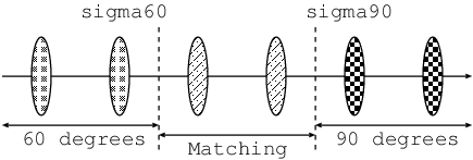 Figure 1
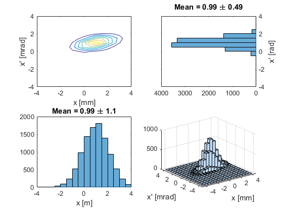 Figure 2
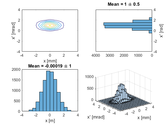 Figure 3
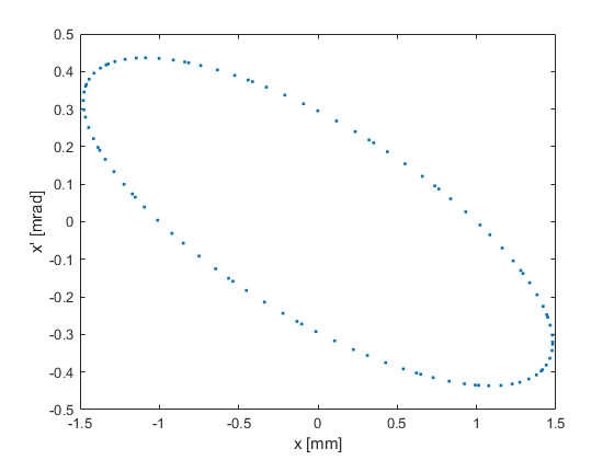 Figure 4
 Figure 5
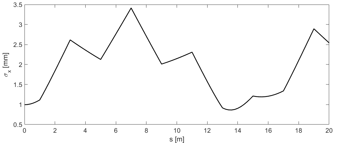 Figure 6
Peer Reviews
No public reviews on file for this paper yet. If you reviewed it on a platform where reviews are public (OpenReview, ICLR, NeurIPS, ICML), you can paste yours below so the community can read it here.
Videos
No videos yet. Explain this paper in a talk, walkthrough, or lecture? Add one.
Taxonomy
TopicsParticle Accelerators and Free-Electron Lasers · Particle accelerators and beam dynamics
Beam Optics Primer
using Octave or MATLAB
V. Ziemann, Uppsala University
(June 16, 2019)
Abstract
This primer provides a basic introduction to beam optics concepts that are commonly used to describe charged particle accelerators.
1 Introduction
The purpose of this document is to prepare the reader for the tutorial sessions on the forthcoming CERN Accelerator School (CAS), where basic methods for beam optics calculations will be illustrated with the help of Octave[1], MATLAB [2], or Python [3]. At the school, the students will be asked to “play around” with the software and then use it to solve simple beam optics problems. This initial familiarization with the basic concepts and the software helps to maximize the benefit drawn from the tutorial sessions at CAS. Note that this report addresses the absolute newcomer.
We start by introducing some basic theoretical concepts first, but illustrate the ideas with, often trivial, examples in Octave as we go along. Exercises are interspersed in the text and readers, especially newcomers to the field, are encouraged to solve them. We will discuss the solutions at CAS.
This document focuses on Octave/MATLAB, loosely following [4], but a version of this report [5], in which all examples are based on Python [3], will be available. Most examples in the earlier parts of this tutorial are based on one transverse dimension.
2 Ray tracing
The motion of charged particles with respect to the center of the beam pipe in an accelerator conceptually resembles the motion of optical rays with respect to the optical axis. In the latter case, a ray at a given longitudinal position is characterized by its distance and its angle with respect to the optical axis. In the absence of lenses or prisms, the light ray (I normally visualize the ray from a laser pointer) moves on a straight line. Its distance to the optical axis at a downstream location therefore changes according to where we assume that is the distance between where the ray’s coordinates are and where the coordinates are Since it moves on a straight line, the angle does not change from to such that we have The two equations for and can be combined in a single equation,
[TABLE]
where the motion from to is encapsulated in the matrix.
- •
Exercise 1: Show that multiplying two such matrices, one with and the other with in the upper right corner, produces a matrix with the sum of the distances in the upper right corner.
When a ray passes a focusing (thin) lens, its angle changes proportional to the transverse distance of the ray from the center of the lens, which we assume to be aligned with the optical axis. Recall the definition of the focal length, which requires a lens to deflect all parallel rays, independent of their transverse position, in a such a way, that the rays cross the optical axis at the same point—the focal point. This point is located a distance the focal length, downstream of the lens. We therefore require that the change of angle in the lens is given by Since we assumed the lens to be very thin, the transverse position of the ray does not change and we have Here we assumed that the coordinates of the rays, immediately upstream of the lens are and immediately downstream they are Note that also these two equations can be combined into the following matrix-valued equation
[TABLE]
where a describes a focusing lens and a defocusing lens.
- •
Exercise 2: How do you describe a ray that is parallel to the optical axis?
- •
Exercise 3: How do you describe a ray that is on the optical axis?
- •
Exercise 4: Show by multiplying the respective matrices that a parallel ray, which first passes through a lens with focal length and then moves on a straight line, actually crosses the optical axis at a distance downstream of the lens. Hint: think a little extra about ordering of the matrices!
A preliminary analysis of optical systems can easily be described by the matrices, they are called Ray- or ABCD-matrices in the optics literature [6]. But optics is not exactly our topic, and we will therefore turn to charged particles, instead.
As a matter of fact, we can describe the motion of charged particles in the presence of magnetic lenses by the same mathematical framework, namely with matrices; in accelerator physics they are usually referred to as transfer matrices. We only have to establish a few correspondences beforehand. For charged particles, the optical axis can be visualized as the center of the beam pipe. Moreover, at a longitudinal position a particle can also be characterized by its distance and and angle with respect to the center of the beam pipe. Here, we need to point out that for charged particles this description is valid for moderately small angles which is called the paraxial approximation and is valid for angles in the range of a few tens of mrad. But this is usually valid in accelerators—10 mrad correspond to a change of distance of 10 mm per meter!
In the absence of external influences—this can be visualized as a piece of beam pipe without magnets—charged particles also move on a straight line. The matrix that maps position and angle from one end of the empty pipe to the other end is the same we used for light rays and is given in Equation 1. This matrix is commonly referred to as the matrix for a drift space and the empty piece of beam pipe is referred to as a drift space.
The elements corresponding to the optical lenses are magnetic elements with a magnetic field that depends linearly on the transverse position Note the resemblance with the light rays: all parallel rays have to go through the focal point downstream and that requires that the deflection angle of each ray has to be proportional to its distance from the optical axis. In the same way must charged particles be deflected more, due to the Lorentz force that the moving particles experience, if they are further from the axis of the magnet. Magnets with the required linearly rising magnetic field are quadrupoles and, if they are moderately short, they can be described by the matrix in Equation 2. Their inverse focal length is directly proportional to the magnetic gradient but we leave the details of the conversion to more advanced texts [4, 7, 8, 9].
We note, however, that the magnetic fields in the quadrupoles have to fulfill Maxwell’s equations. This forces the transverse components and of the magnetic field to obey the curl equation: A linearly increasing field component in one direction causes the other component to decrease. Quadrupoles therefore focus particles in one transverse plane, but defocus the same particles in the other plane. Since we will only consider one plane in this tutorial, we will not encounter this “feature” directly. We will, however, build beam lines consisting of both focusing and defocusing quadrupoles. The motivation to use both types of quadrupoles is to be able to describe the other plane in the beam pipe as well.
There are many more magnets that are used to guide the beam—big dipoles and small steering magnets—and other magnets to correct various effects, but we will, in the early sections of this tutorial, confine ourselves to drift spaces and quadrupoles and will build larger beam optical systems with these elements alone. We will implement most matrix manipulations in software in order to avoid excessive matrix calculations by hand.
3 Software to move particles around
Our task is to follow a particle through a sequence of drift spaces and quadrupoles, modeled by the matrices from Equation 1 and 2. To do so, we first encode the matrices in a convenient way. Here we use octave’s ability to write functions with the help of the @-operator, which specifies the input argument
D=@(L)[1, L; 0, 1];
This command defines a function D() that receives the length L as input and returns the matrix from Equation 1. We can then write D(2)*D(5) at the octave command prompt and should obtain a matrix with 7 in the upper right corner. Likewise, we define the function Q()
Q=@(F)[1, 0; -1/F, 1];
which returns the matrix from Equation 2. We also note that the column vector with can be expressed as
X0=[x; xp];
where the semicolon separates rows in a vector or matrix, and a comma separates the columns. The semicolon at the end of a command suppresses displaying the result of the assignment or the calculation.
- •
Exercise 5: Set F=3 and numerically verify what you found in Exercise 4, namely that parallel rays cross the axis after a distance
Using these matrices it is straightforward to find out what the transverse coordinates of a ray that enters the system at one end will be, once it reaches the other end. To make this analysis more efficient we need a language to describe beam lines with many elements.
We encode the description of the beam line in a matrix, whose first column contains a code: we use 1 for a drift space and 2 for a quadrupole. The second column contains a repeat code, which is mostly for cosmetic reasons in order to make plots look smoother. A number 10 simply instructs the software to repeatedly apply the matrix for that element ten times. The third column contains the length of the element and the fourth column contains an additional parameter; for a quadrupole, for example, it will contain its focal length. An example of such a beam-line description is the following
F=2.5; fodo=[1, 5, 0.2, 0; 2, 1, 0, F; 1, 10, 0.2, 0; 2, 1, 0, -F; 1, 5, 0.2, 0];
which first defines the focal length F to be 2.5 m and then defines an array, called fodo that follows the conventions defined above. The first line describes 5 segments of a drift space, each being 0.2 m long. The second line describes a quadrupole that is not segmented and therefore only has the repeat-count of 1. Moreover, the quadrupole is thin and has the length zero in the third column and the focal length in the fourth. The third line describes a drift space, consisting of ten segments with length 0.2 m each. The fourth line, again with code 2 in the first column, describes a second quadrupole, this time with a negative focal length. The last line is equal to the first one. We call the array that describes our beam line fodo, because it consists of an alternating sequence of focusing (F) and defocusing (D) quadrupoles, separated by not-focusing (O) drift spaces. FODO-based beam lines are very common, for example, the arcs of the LHC are based on them. The reason to alternate the quadrupole polarity is to focus in both transverse planes equally, despite the each quadrupole treating the two planes in the opposite manner.
- •
Exercise 6: Recall that the imaging equation for a lens is which corresponds to a system of one focusing lens with focal length sandwiched between drift spaces with length and respectively. Write a beam-line description that corresponds to this system. We will later return to it and analyze it.
Having a description of sequence of elements in a beam line available, we now will turn to assembling all matrices that map the coordinates of a particles at the start of the beam line to each and every beam-line element. This will allow us to follow a particle on its journey through the accelerator.
First we have to take care of some accounting and use the following code to accomplish that.
beamline=fodo; nlines=size(beamline,1); nmat=sum(beamline(:,2))+1; Racc=zeros(2,2,nmat); Racc(:,:,1)=eye(2); spos=zeros(nmat,1);
We use the convention to call the beam line beamline in the software. In this way we can simply redefine beamline if we want to analyze a different one. Then we also need the number of lines nlines in the beam-line description. We just use the size of the first dimension of beamline, which is the number of rows; for fodo this would be 5. We also need the number of matrices nmat we will have to calculate, which depends on the repeat-count in the second column of beamline. We simply add these number and add one to place a unit matrix in the first location, which makes array handling more convenient. Then we allocate space for all the matrices Racc; we create an array of nmat matrices filled with zeros. Note that each matrix will eventually contain the transfer matrix from the start of the beam line up to the location immediately after each segment. We fill the first matrix with a unit matrix, which is denoted by eye(2) in octave or MATLAB. Finally, we allocate the array spos that will be filled with the longitudinal position of the end point of each segment. This will allow us to make plots with the horizontal axis denoting the longitudinal position, rather than the sequence number of the segment.
With the accounting out of the way, we are now ready to assemble the transfer matrices with the following code
ic=1; % element counter for line=1:nlines % loop over input elements for seg=1:beamline(line,2) % loop over repeat-count ic=ic+1; % next element Rcurr=eye(2); % matrix in next element switch beamline(line,1) case 1 % drift Rcurr=D(beamline(line,3)); case 2 % thin quadrupole Rcurr=Q(beamline(line,4)); otherwise disp(’unsupported code’) endΨΨ Racc(:,:,ic)=Rcurr*Racc(:,:,ic-1); % concatenate spos(ic)=spos(ic-1)+beamline(line,3); % position of element end end
We first initialize the element counter ic, which helps us to keep track of all the segments in the beam line. Then we loop over the lines in the beam-line description beamline and then, in a second loop, over the repeat-count. The first thing we do is incrementing the element counter ic and initialize the matrix for the current segment Rcurr to the unit matrix eye(2). The switch statement branches, depending on the code number in the first column of the current line, which denotes the type of element. If the code is 1, we copy the matrix for a drift space with length given by the third column beamline(line,3) to Rcurr. If the code is 2, we copy the matrix for a quadrupole with its focal length specified in the fourth column to Rcurr. If the first column contains anything else, we write a short note to the display. At this point, Rcurr contains the appropriate matrix for the currently considered segment and we left-multiply it to the matrix Racc(:,:,ic-1) that ends just upstream of the current segment and we then store the result in Racc(:,:,ic). This procedure will recursively assemble all matrices in Racc. Likewise, we add the length of the current segment to spos, which is successively filled with the positions at the exit of each segment. Once the loops have finished, Racc will contain all matrices that map the coordinates of a particle at he start of the beam line to the exit point of each segment and spos tells us where along the beam line that point is.
Note that for future use, we encapsulate most of the functionality to allocate memory for the transfer matrices and the actual calculation of the matrices in a separate function calcmat(), which receives the beamline as input and returns the matrices and some accounting information in the following form:
[Racc,spos,nmat,nlines]=calcmat(beamline)
The code for calcmat(), which is very similar to beamoptics.m, is reproduced in Appendix B.
Now we are ready to use this code. As example, we map the initial coordinates x0, specified as a column vector, along the beam line and plot the transverse position x as a function of the longitudinal position
x0=[0.001;0]; % 1 mm offset at start data=zeros(1,nmat); % allocate memory for k=1:nmat x=Racc(:,:,k)x0; data(k)=x(1); % store the position end plot(spos,1e3data,’k’); xlabel(’s [m]’); ylabel(’ x [mm]’);
After x0 is defined, we allocate the array data to contain the variables we want to display. Then we loop over all the segments in the beam line, of which there are nmat. In the loop, we multiply the initial coordinate x0 with transfer matrix to the exit of each segment, which is stored in Racc. Since we want to display the transverse position, we copy the position x(1) to data, which will automatically have the same array dimensions as spos, such that we can plot the transverse position as a function of spos. Note that we multiply the contents of data by in order to convert it to mm, which is also annotated in the axes labels.
- •
Exercise 7: Prepare initial coordinates that describe a particle that is on the optical axis, but has an initial angle and plot the position along the beam line.
- •
Exercise 8: Plot the angle along the beam line.
The code only shows the trajectory in a single FODO cell. If we want to display the trajectory, for example, through five consecutive cells, we only have to replace the definition of the beamline early in the file by
beamline=[fodo;fodo;fodo;fodo;fodo];
where we must use the semicolon as a separator, because we need to stack the beam line descriptions one after the other and thereby create more lines. Optionally, we can replace the previous command by
beamline=repmat(fodo,5,1);
where we use the built-in command repmat.
- •
Exercise 9: Plot both the position and the angle through five cells.
- •
Exercise 10: Plot the position through 100 cells, play with different values of the focal length F and explore whether you can make the oscillations grow.
- •
Exercise 11: Use the beam line for the imaging system you prepared in Exercise 6 and launch a particle with and an angle of mrad at one end. Verify that this particle crosses the center of the beam pipe at the exit of the beam line, provided that and satisfy the imaging equation that is shown in Exercise 6.
Up to now the software allows us to map single particles through a beam line. But a beam consists of more than a few particles and we have to have a look at how to describe such ensembles of particles.
4 Many particles, the beam
Each of the many particles in a beam has its individual coordinates Under most circumstances are the positions and angles distributed according to a normal, or Gaussian, distribution. We create the coordinates of particles as a array beam that we fill with normally distributed random numbers with the help of the built-in function randn(). The following commands can be found in the script propagate_beam.m.
Npart=10000; beam=randn(2,Npart);
These random numbers have a mean of zero and unit rms, such that we scale them by multiplying the first coordinate by the rms beam size sigx and the second coordinate by the rms angular divergence sigxp.
sigx=1; x0=0; % 1 mm beam size and offset x0 sigxp=0.5; xp0=1; % 0.5 mrad angular divergence and initial angle xp0 beam(1,:)=sigxbeam(1,:)+x0; beam(2,:)=sigxpbeam(2,:)+xp0;
where we also introduce the initial offsets x0 and xp0, which are then the respective means of the distribution. We can now verify that the distribution has the desired properties by calculating the beam_position and the beam_size via
beam_position=mean(beam(1,:); beam_size=std(beam(1,:))
where beam(1,:) refers to the first row of the matrix beam, which contains the positions of all particles. The built-in functions mean() and std() return the average and rms of the distribution, respectively.
- •
Exercise 12: Calculate the angular divergence of the beam.
We can visualize the particle distribution by plotting one and two-dimensional histograms and contour plots. We encapsulate the code in the function show_beam(). The function, shown in its entirety in the appendix, receives the array beam with the coordinates and the desired bin spacing for the histograms as input. It then creates four subplots: the top left shows a contour plot of the distribution in and the plots immediately to the right and below the contour plot show the histograms with the projections onto the respective axes, and in the bottom right a two-dimensional histogram is displayed.
We then use a transfer matrix R to propagate the beam to a downstream location, here through a drift space with a length of 1 m, by multiplying the beam with R , as shown in the following example.
R=[1,1;0,1]; % drift space with L=1 m beam=R*beam; % propagate particles
Calling show_beam() again produces the plot on the right-hand side in Figure 1. We find that the contour plot has slightly changed shape; the ellipses have rotated. Moreover, the mean of the horizontal distribution has changed to 1 mm. This is a consequence of the initial angle mrad, which caused the beam to move towards the positive x-axis by 1 mm over the 1 m long drift space. The horizontal width has increased to 1.1 mm.
Note that we specified the transverse dimensions and angle in mm and mrad instead of m and rad. This is permissible, because transfer matrices describe a linear transformation, and multiplying the vector to the right by some number, here causes the output on the left of the matrix multiplication to be scaled by the same number.
- •
Exercise 13: Try this out yourself: Scale the input vector by 17 times the month of your birthday (85 if you are born in May) and verify that the output vector from the matrix multiplication has changed by the same factor.
We will continue to use mm and mrad for the transverse coordinates and will now calculate the beam size after every segment in the beam line. We use beamoptics.m to build a beam line of five consecutive FODO cells and prepare all transfer matrices Racc. Then we execute the following code:
beam0=beam; % copy initial distribution to beam0 data=zeros(nmat,1); % allocate space for plotting for k=1:nmat beam=Racc(:,:,k)*beam0; % propagate beam0 data(k,1)=std(beam(1,:)); % calculate rms beam size end plot(spos,data(:,1),’k’) % plot along the beam line xlabel(’s [m]’); ylabel(’\sigma_x [mm]’)
First we copy the beam distribution to beam0 in order to avoid overwriting it. Then we allocate some space to store the values we intend to display and then loop over all elements in the beam line. At each step in the loop, we propagate the initial beam0 to the new location in the beam line and store the rms of the positions of all particles in data. After the loop completes, we display the beam size as a function of and annotate the axes. Figure 2 shows the resulting plot. We observe that the beam size grows over the first meter, where it traverses a defocusing quadrupole, which increases the beam size further until at m. There the first focusing quadrupole reduces the beam size until the defocusing quadrupole at m increases the beam size again, whence the focusing quadrupole at m reduces it again; and so forth. We also observe that the beam0 we initially prepared can become larger up to an rms beam size of a little under mm.
- •
Exercise 14: Display (a) the average position of the particles along the beam line. Likewise, display (b) the angular divergence.
- •
Exercise 15: What happens if you (a) reduce or (b) increase the initial angular divergence sigxp by a factor of two?
Normally, one is not really interested in the histogram of the particle distribution. Information about the centroid position, the beam size, and possibly the angular divergence are enough. So, wouldn’t it be nice, if we could move the interesting quantities around, instead of thousands of sample particles? It turns out that this is possible and that is the topic of the next section.
5 Moving beams around
To simplify the writing of many matrix-valued equations, we introduce the notation that the position is denoted by and the angle by This allows us to express the propagation of the particle coordinates as If we have to deal with many particles we label them by a second subscript, separated from the first by a comma; is thus the angle of particle number 17.
When we calculated the average beam position using the built-in functions, the software actually performed the following operations
[TABLE]
where the index sums over the particles. The notation with the angle brackets denotes thus averaging over the ensemble of particles. We also introduced the quantities and to denote the averages. Likewise, the rms quantities are calculated via
[TABLE]
By inspection, we should not be surprised that there is also a third variant of the above sums, given by
[TABLE]
which describes the correlation between position (index 1) and angle (index 2). This quantity is actually capable of describing the rotation of the contour in the right-hand plot in Figure 2 that showed up after propagating the initial beam through a 1 m long drift space.
These five quantities and describe all the interesting properties of a beam. Note that and are the first moments of the two-dimensional beam distribution and the with are the three independent second moments; actually they are the central moments, because they describe the second moments with respect to the centroids. Note that usually the three independent second moments can be written to form a symmetric –matrix that is given by
[TABLE]
with We use the convention that sigmas without subscripts denote the matrix and sigmas with subscripts denote the matrix elements. We also point out that the sigma matrix changes from one location in the beam line to another location Remember that Figure 2 shows the beam size as a function of along the beam line.
In the more advanced literature [4, 7], but also in Appendix A, it is shown that the first and second moments propagate according to
[TABLE]
where denotes the column vector with entries and at longitudinal location The first equation describes the remarkable fact that the centroid of the beam—the first moments—propagate in the same way as single particles. The second equation describes the propagation of the beam matrix, as defined in Equation 6. In Equation 7 we use the common convention to denote the transpose of the matrix by
The two equations in Equation 7 are particularly convenient and efficient to implement in software, because they just describe matrix multiplication of the centroid and the sigma matrix , both of which describe the beam, and the transfer matrices which describe the hardware of the beam line. We can now implement these equations in the software by adding the following lines after the code from page 4, which is re-used to define the initial beam and assemble the transfer matrices Racc. The following code segment then adds the calculations according to Equation 7.
X0=[0;xp0]; % 1 mrad initial angle sigma0=[sigx^2,0;0,sigxp^2]; % initial sigma matrix for k=1:nmat X=Racc(:,:,k)X0; % Equation 7 sigma=Racc(:,:,k)sigma0Racc(:,:,k)’; data(k,2)=sqrt(sigma(1,1)); end plot(spos,data(:,1),’k’,spos,data(:,2),’’) xlabel(’s [m]’); ylabel(’\sigma_x [mm]’)
In this code segment, we first initialize the centroid X0 and the sigma-matrix sigma0 with the same values used on page 4. Then we loop over the nmat positions in the beam line and propagate both centroid and sigma-matrix according to Equation 7. In this example we only store the beam size in the second column of data. After the loop completes, we plot both the newly calculated beam sizes and those calculated previously as a function of spos. The result, displayed in Figure 3, shows very good agreement of the beam sizes. Henceforth, we will only use Equation 7 for propagating beams through beam lines.
- •
Exercise 16: Using Equation 7, display (a) the average position of the particles along the beam line. Likewise, (b) display the angular divergence. Compare with the result you found in Exercise 14.
- •
Exercise 17: Can you find an initial beam matrix sigma0 that reproduces itself at the end of the beam line?
In Figure 3 the beam size oscillates in a somewhat uncontrolled fashion along the beam line. Next we will explore whether we can find periodic oscillations that repeat after each cell.
6 Periodic systems and beams
To explore the periodicity of a beam optical system, we first consider a single FODO cell only and follow a single particle with initial coordinates x=[1;0] over a large number of turns, as shown in the following script
% trak_single_particle.m beamoptics; % with beamline=fodo; Nturn=100; data=zeros(Nturn,2); x=[1;0]; % initial condition, 1 mm, no angle for k=1:Nturn x=Racc(:,:,end)*x; data(k,1)=x(1); data(k,2)=x(2); end plot(data(:,1),data(:,2),’.’) xlabel( ’x [mm]’); ylabel(’x’’ [mrad]’)
Before running this script, we have to update beamoptics.m to prepare matrices for a single cell by defining beamline=fodo, such that calling beamoptics makes all matrices available to the script shown on this page. After specifying the requested number of turns Nturn and allocating the array data, we start the loop. Inside the loop, we use the present coordinates x, map them through one turn by multiplying with the transfer matrix Racc(:,:,end), and store the coordinates in the same vector x, which is thereby continuously updated with the coordinates turn after turn. In each turn, we also save the coordinates to data for later display. After the loop has finished, we plot the first column of data, which contains the positions on consecutive turns, versus the second column, which contains the angle on the corresponding turns. The plot, shown in Figure 4, displays an ellipse.
- •
Exercise 18: Explore different initial coordinate and compare the phase-space plots you obtain.
- •
Exercise 19: Execute plot(data(:,1)) to observe the turn-by-turn positions. What do you observe?
- •
Exercise 20: In the definition of fodo at the top of beamoptics.m reverse the polarity of both quadrupoles and prepare a phase-space plot. How does it differ from the one in Exercise 18?
- •
Exercise 21: Prepare an array describing a FODO cell that starts immediately following the quadrupole with the negative focal length and prepare the phase-space plot.
The particle, performing stable oscillations reminiscent of a harmonic oscillator, suggests that we can split the transfer matrix for one turn into a product of three matrices [4]; a rotation matrix, sandwiched between two matrices that distort the coordinates
[TABLE]
Here and are two, presently undetermined, parameters that describe the distortion. We can, however, determine them from by comparing coefficients with the result
[TABLE]
These equations are encapsulated in the following function R2beta()
function [Q,alpha,beta,gamma]=R2beta(R) mu=acos(0.5*(R(1,1)+R(2,2))); if (R(1,2)<0) mu=2pi-mu; end Q=mu/(2pi); beta=R(1,2)/sin(mu); alpha=(0.5*(R(1,1)-R(2,2)))/sin(mu); gamma=(1+alpha^2)/beta;
which allows us to determine the parameters and from any transfer matrix that permits stable oscillations. Note that this is only possible for which indicates the limit of stability.
- •
Exercise 22: Find the range of focal lengths F for which the FODO cells permit stable oscillations.
The parameters returned by R2beta() are commonly called the phase advance the Twiss parameters and and is called the tune.
So, why did we analyze the transfer matrix if we actually want to construct a sigma matrix that is periodic? Because the Twiss parameters make it particularly simple to build a beam matrix sigma0 that is repeats itself after one cell. It is given by
[TABLE]
where we introduced the emittance whose relevance will become obvious in a short while. We can now propagate the matrix through the cell and use Equation 8 to express the transfer matrix through and After some algebra, we find
[TABLE]
which shows that the beam matrix, as defined in Equation 10, reproduces itself after one cell. Let’s try out whether this really works in the following code.
% periodic_beam.m beamoptics; % with beamline=fodo; [Q,alpha,beta,gamma]=R2beta(Racc(:,:,end)); data=zeros(nmat,1); % allocate memory for display eps=1; % set emittance to unity sigma0=eps*[beta, -alpha;-alpha,gamma]; for k=1:nmat sigma=Racc(:,:,k)sigma0Racc(:,:,k)’; data(k,1)=sqrt(sigma(1,1)); end plot(spos,data(:,1),’k’)
Here we call beamoptics to prepare the transfer matrices and then R2beta() to calculate the Twiss parameters, from which we build the initial beam matrix sigma0 that is subsequently propagated through the beam line.
- •
Exercise 23: Run periodic_beam and convince yourself that the sigma matrix at the end of the cell is indeed equal to sigma0.
- •
Exercise 24: Write down the numerical values of initial beam matrix sigma0, then build a beam line made of 15 consecutive cells by changing the definition of beamline in beamoptics.m and then, using sigma0 with the noted-down numbers, prepare a plot of the beam sizes along the 15 cells. Is it also periodic?
The emittance that appeared in Equation 10 as an arbitrary constant is actually conserved when propagating the beam matrix, which is easily seen from
[TABLE]
for an arbitrary transfer matrix because all transfer matrices have unit determinant. This is true for all maps that describe the motion of a beam through static magnetic fields, in particular, for the matrices for drift space and quadrupole and therefore also for products of those elements.
- •
Exercise 25: Verify that all matrices Racc(:,:,k) have unit determinant.
Note also that the matrix with the Twiss parameters and which appears in Equation 10, has unit determinant by construction. The Twiss parameters and describe the relative magnitude of the matrix elements in and the emittance determines the absolute magnitude of the beam. In particular, when considering the 11-element of a sigma matrix, we see that the absolute beam size is given by Here the emittance is constant and sets the scale, whereas describes the modulation of the beam size along a beam line from one position to another.
- •
Exercise 26: Multiply sigma0 from Exercise 24 by 17 and calculate the emittance. Then propagate the sigma matrix through the beam line from Exercise 24 and verify that the emittance of the sigma matrix after every element is indeed constant and equal to its initial value.
Up to now, we have used FODO cells and calculated the phase advance and the Twiss parameters from the transfer matrices. We now reverse the procedure and try to find hardware parameters, such as the focal length of a quadrupole, to achieve certain, desirable values. This procedure, commonly called matching, is the topic of the next section.
7 Satisfying one’s desires: matching
From the analysis of large circular accelerators it is known that an important parameter for the stability of periodically traversed beam lines is the phase advance of a cell, or the tune which is the phase advance for the whole ring, divided by Let us consider a single cell first and try to adjust the focal length F of the quadrupoles to a value, such that the phase advance of the cell is which corresponds to The following short script first defines F and fodo, then calls calcmat() to calculate the transfer matrices, and finally uses the last one Racc(:,:,end) as argument for R2beta(), which returns the phase advance and the Twiss parameters.
% match_phase_advance.m clear all; close all F=2.5; % focal length of the quadrupoles fodo=[ 1, 5, 0.2, 0; 2, 1, 0.0, -F; 1, 10, 0.2, 0; 2, 1, 0.0, F; 1, 5, 0.2, 0]; beamline=fodo; [Racc,spos,nmat,nlines]=calcmat(beamline); [Q,alpha,beta,gamma]=R2beta(Racc(:,:,end)); Q=Q
The statement Q=Q serves only to display the value of Q which is the sought-after phase advance divided by
- •
Exercise 27: Vary F by hand and try to (a) find a value that returns (b) Then try to find a value of F that produces a phase-advance. What is the corresponding value of ?
This procedure mimics the matching done by the accelerator-design software. There a minimizer optimizes a cost-function that encodes the desired constraints. In Exercise 27 you have to do it by hand.
A common task when designing accelerators is matching one section of a beam line to another one. Here we will assume that the upstream beam line consists of FODO cells with a phase advance and the downstream beam line of FODO cells with a phase advance. These are the cells with the focal length we calculated in Exercise 27. In between the and we place a third cell with two quadrupoles that we will use to match the upstream to the downstream beam line. To do so, we need to prepare periodic beam matrices sigma60 and sigma90 for the respective sections. Note that sigma90 only depends on two parameters: the Twiss parameters and and therefore we also need two quadrupoles with independently variable focal length to adjust until the final beam matrix equals sigma90. See Figure 5 for an illustration of the geometry.
- •
Exercise 28: Implement the procedure described in the previous paragraph.
The discussed matching tasks are only basic examples of the tasks encountered when designing an accelerator. As mentioned before, most software packages have a more or less convenient way to specify the constraints to fulfill and the magnets to vary to satisfy the constraints. Then the software automatically produces the magnet settings.
8 …and beyond…
So far we only considered the very basic optical elements and confined ourselves to a single transverse dimension. During CAS we will build on these basics and extend the software in several directions. In this section, we therefore give some indication of things to come. We start by including quadrupoles that have a finite length. In the introductory beam optics lectures you will learn that the matrix for these elements depends on the polarity of the magnet excitation, as specified by a parameter The matrix is given by
[TABLE]
and
[TABLE]
and this brings us directly to
- •
Exercise 29: Include these matrices in calcmat() and assign code 5 to them. Hint: write an external function that returns and call it from calcmat().
Once the software is able to handle long quadrupoles, we can replace the thin quadrupoles in the beam-line description used earlier.
- •
Exercise 30: Use the beam line from Exercise 27 (60 degrees/cell FODO) and replace the thin quadrupoles by long quadrupoles with a length of 0.2, 0.4, 1.0 m. Make sure the overall length and the phase advance of the FODO cell remains unchanged. By how much does the periodic beta function at the start of the cell change? Express the change in percent.
In the introductory optics lectures you will learn that a so-called sector dipole magnet will exhibit weak focusing in the bending plane. The transfer matrix for this magnet will be shown to be
[TABLE]
- •
Exercise 31: Include this matrix in calcmat() and assign the code 4 to it.
- •
Exercise 32: Insert 1 m long dipoles in the center of the drift spaces of the FODO cells from Exercise 27 while keeping the length of the cell constant. Investigate deflection angles of and degrees. Check by how much the periodic beta functions change. Why do they change? Explain! Can you compensate the phase advance by adjusting the strength or focal lengths of the quadrupoles?
All matrices discussed up to now only address one transverse plane and assume that all particles have the same momentum .
But this is only approximately true in a real accelerator and we therefore must take small momentum deviations into account. Instead of describing a particle by its transverse coordinates alone, we now characterize each particle by which requires to upgrade the transfer matrices to matrices that operate on state vectors The matrix for a drift space therefore turns out to be
[TABLE]
with the original matrix from Equation 1 in he top left corner, a in the bottom right corner and zeros in the other positions of the third row and the third column. The transfer matrices for thin and long quadrupoles are updated likewise. Only the matrix for the sector dipole has non-zero entries in the third column
[TABLE]
In order not to mix functions with the same name, but using instead of matrices, prepare a subdirectory for the upgraded matrices.
- •
Exercise 33: Upgrade the software to consistently handle matrices for drift space, quadrupoles, and sector dipoles.
- •
Exercise 34: Build a beam line of six FODO cells with a phase advance of 60 degrees/cell (thin quadrupoles are OK to use) and add a sector bending magnet with length 1 m and bending angle degrees in the center of each drift. You may have to play with the quadrupole values to make the phase advance close to 60 degrees. But you probably already did this in Exercise 32.
- •
Exercise 35: Use the starting conditions and plot the position along the beam line. Repeat this for and for . Plot all three traces in the same graph. Discuss what you observe and explain!
We also need to upgrade the beam matrix to be consistent with the transfer matrices. It is then a matrix itself with the original sigma-matrix from Equation 6 in the top-left corner, zeros in the third column and row, except the matrix element in the lower-right corner, which contains the square of the momentum spread
- •
Exercise 36: Work out the transverse components of the periodic beam matrix . Assume that the emittance is meter-rad. Furthermore, assume that the momentum spread is zero and plot the beam size along the beam line.
- •
Exercise 37: Plot the beam size for for and for . What happens if you change the phase advance of the cell? Try out by slightly changing the focal lengths.
- •
Exercise 38: Determine the periodic dispersion at the start of the cell. Then plot the dispersion in the cell.
For these exercises you definitely need to consult the slides from the introductory beam optics lectures for background information.
Instead of adding the momentum deviation as additional degree of freedom for the simulation, we can extend the simulation to comprise of both transverse degrees of freedom, the horizontal and the vertical plane. The matrices that describe the dynamics are then matrices with the matrices for the respective planes filling the upper-left and the lower-right sub-matrices. As an illustration, we show the matrix for a focusing () quadrupole
[TABLE]
where is the matrix from Equation 13, from Equation 14, and is the matrix containing only zeros. For the sub-matrices and are exchanged. The matrix for a thin quadrupole is constructed likewise. From the introductory lectures, we know that the matrix for sector dipole only shows weak focusing in the horizontal plane, but behaves as a drift space in the vertical plane. Its matrix is therefore given by
[TABLE]
where is the matrix from Equation 15 and the matrix for a drift space from Equation 1. Note that in this framework, we assume that all particles have the reference momentum and we can therefore ignore the momentum deviation
- •
Exercise 39: Convert the code to use matrices, where the third and fourth columns are associated with the vertical plane. Create a separate subdirectory for the calculations with the matrices.
Using this software to address the following exercises. Note that changing a quadrupole simultaneously affects the phases advances and the beta functions in the respective planes.
- •
Exercise 40: Start from a single FODO cell with 60 degrees/cell you used earlier. Insert sector bending magnets with a bending angle of degrees in the center of the drift spaces. The bending magnets will spoil the phase advance in one plane. Now you have two phase advances and need to adjust both quadrupoles (by hand to 2 significant figures) such that it really is 60 degrees in both planes.
- •
Exercise 41: Use the result from exercise 2 and adjust the two quadrupoles such that the phase advance in the horizontal plane is 90 degrees, cell, while it remains 60 degrees/cell in the vertical plane.
- •
Exercise 42: Prepare a beam line with eight FODO cells without bending magnets and with 60 degrees/cell phase advance in both planes. (a) Prepare the periodic beam matrix sigma0 (4x4, uncoupled) as the initial beam and plot both beam sizes along the beam line. (b) Use sigma0 as the starting beam, but change the focal length of the second quadrupole by 10 % and plot the beam sizes once again. Discuss you observations.
- •
Exercise 43: From the lecture about betatron coupling identify the transfer matrix for a solenoid and write a function that receives the longitudinal magnetic field and the length of the solenoid as input and returns the transfer matrix. Then extend the simulation code to handle solenoids. Finally, define a beam line where you place the solenoid in the middle of a FODO cell and follow a particle with initial condition What do you observe? Is the motion confined to the horizontal plane?
And this brings us to the end of this tutorial. Here, we try to give some idea about what goes on “under the hood” of full-blown beam optics codes, such as MADX [10]. Moreover we hope to have provided some guidance on how to write such a simulation code yourself and how to use it to “play around” with simple beam-optical system and gets a feeling for their behavior. But the story does not stop here. There are many more topic covered in the CERN Accelerator School and the more advanced textbooks [4, 7, 8, 9].
Appendix A Propagating the moments of a distribution
Here we work out how the moments propagate through the beam line as a function of the transfer matrix that maps particle coordinates from one place to another. If we assume that the downstream coordinates are given by with and the upstream coordinates by Note that here subscript labels the position and the angle. The equation that relates to can then be written as which is valid for every particle in the ensemble. We can therefore calculate the averages over the final distribution as
[TABLE]
Here the first equality is simply the definition of and the second follows from replacing the particle coordinates through the transfer matrix elements and the upstream coordinates Since the same matrix applies to all particles, we can pull it out of the averaging, likewise with the summation over But then we are left with the averages of which is the same as This simple calculation proves the remarkable fact that the beam centroids propagate in the same way as individual particles and we can visualize the beam centroid as some sort of super-particle. Note, however, that this feature depends crucially that the propagation is described by a linear operation—a matrix multiplication. If non-linear elements, such as sextupoles are present in the beam line, this correspondence is no longer strictly true!
Now we consider the second moments, but assume that the centroids are zero which simplifies the notation. The sigma-matrix elements “on the other end of the transfer matrix ” can be calculated in the following way
[TABLE]
where the first equality follows from inserting in the definition of . Since the transfer matrices are constant and summing is linear, we can extract both sum and from the averaging, denoted by the angle brackets and find that the sigma matrix transform according to
[TABLE]
where we converted the expression from Equation 21, which is given in components, into a matrix equation. Note that denotes the transpose of the matrix Equations 20 and 22 are given in Equation 7 in Section 5 in the main part of the text.
Appendix B Octave/MATLAB code
B.1 beamoptics.m
This script is used in Section 3 to plot the trajectory of a particle. It is already explained in the main part of the text.
% beamoptics.m, clear all; close all D=@(L)[1, L; 0, 1]; Q=@(F)[1, 0; -1/F, 1]; F=2; % focal length of the quadrupoles fodo=[ 1, 5, 0.2, 0; % 5* D(L/10) 2, 1, 0.0, -F; % QD 1, 10, 0.2, 0; % 10* D(L/10) 2, 1, 0.0, F; % QF/2 1, 5, 0.2, 0]; % 5* D(L/10) %beamline=fodo; % name must be ’beamline’ %beamline=[fodo;fodo]; beamline=repmat(fodo,100,1); nlines=size(beamline,1); % number of lines in beamline nmat=sum(beamline(:,2))+1; % sum over repeat-count in column 2 Racc=zeros(2,2,nmat); % matrices from start to element-end Racc(:,:,1)=eye(2); % initialize first with unit matrix spos=zeros(nmat,1); % longitudinal position ic=1; % element counter for line=1:nlines % loop over input elements for seg=1:beamline(line,2) % loop over repeat-count ic=ic+1; % next element Rcurr=eye(2); % matrix in next element switch beamline(line,1) case 1 % drift Rcurr=D(beamline(line,3)); case 2 % thin quadrupole Rcurr=Q(beamline(line,4)); otherwise disp(’unsupported code’) endΨΨ Racc(:,:,ic)=Rcurr*Racc(:,:,ic-1); % concatenate spos(ic)=spos(ic-1)+beamline(line,3); % position of element end end x0=[0.001;0]; % 1 mm offset at start data=zeros(1,nmat); % allocate memory for k=1:nmat x=Racc(:,:,k)x0; data(k)=x(1); % store the position end plot(spos,1e3data,’k’,’LineWidth’,2); xlabel(’s [m]’); ylabel(’ x [mm]’); xlim([spos(1),spos(end)])
B.2 calcmat.m
The function calcmat() encapsulates the allocating of matrices and the calculation of the transfer matrices Racc in order to avoid rewriting this section over and over. The function receives the beamline as input and returns the matrices Racc, the positions of the elements spos, the number of elements (including all segments), and the number of lines in the beamline.
% calcmat.m, calculate the transfer matrices function [Racc,spos,nmat,nlines]=calcmat(beamline) D=@(L)[1, L; 0, 1]; Q=@(F)[1, 0; -1/F, 1]; nlines=size(beamline,1); % number of lines in beamline nmat=sum(beamline(:,2))+1; % sum over repeat-count in column 2 Racc=zeros(2,2,nmat); % matrices from start to element-end Racc(:,:,1)=eye(2); % initialize first with unit matrix spos=zeros(nmat,1); % longitudinal position ic=1; % element counter for line=1:nlines % loop over input elements for seg=1:beamline(line,2) % loop over repeat-count ic=ic+1; % next element Rcurr=eye(2); % matrix in next element switch beamline(line,1) case 1 % drift Rcurr=D(beamline(line,3)); case 2 % thin quadrupole Rcurr=Q(beamline(line,4)); otherwise disp(’unsupported code’) endΨΨ Racc(:,:,ic)=Rcurr*Racc(:,:,ic-1); % concatenate spos(ic)=spos(ic-1)+beamline(line,3); % position of element end end
B.3 R2beta.m
This function encodes Equation 9. It receives a transfer matrix which is assumed to describe a periodic system, and returns the “tune” or the phase advance divided by , and the Twiss parameters and
function [Q,alpha,beta,gamma]=R2beta(R) mu=acos(0.5*(R(1,1)+R(2,2))); if (R(1,2)<0) mu=2pi-mu; end Q=mu/(2pi); beta=R(1,2)/sin(mu); alpha=(0.5*(R(1,1)-R(2,2)))/sin(mu); gamma=(1+alpha^2)/beta;
B.4 propagate_beam
This function is used to produce the plots in Figure 1,2, and 3.
% propagate_beam.m clear all; close all; % pkg load statistics % only needed for hist3() in octave beamoptics; % with beamline=repmat(fodo,5,1) Npart=10000; beam=randn(2,Npart); x0=0; sigx=1; % initial average position and width xp0=1; sigxp=0.5; % initial angle and divergence beam(1,:)=sigxbeam(1,:)+x0; beam(2,:)=sigxpbeam(2,:)+xp0; xbins=-4sigx:0.5sigx:4sigx; % binning for histogram %ybins=-4sigxp:0.5sigxp:4sigxp; ybins=xbins; beam0=beam; % save for posterity show_beam(beam0,xbins,ybins); % Figure 1 left pause(1); figure R=[1,1;0,1]; beam=R*beam0; show_beam(beam,xbins,ybins); % Figure 1 right figure % Figure 2+3 super-imposed data=zeros(nmat,2); for k=1:nmat % propagate particles beam=Racc(:,:,k)*beam0; data(k,1)=std(beam(1,:)); % data for Figure 2 end X0=[x0;xp0]; % initial centroids sigma0=[sigx^2,0;0,sigxp^2]; % and sigma0 for k=1:nmat X=Racc(:,:,k)X0; % Equation 7 sigma=Racc(:,:,k)sigma0Racc(:,:,k)’; data(k,2)=sqrt(sigma(1,1)); end plot(spos,data(:,1),’k’,spos,data(:,2),’’) xlabel(’s [m]’); ylabel(’\sigma_x [mm]’)
Note that in octave we have to load the statistics package with the command pkg load statistics, which is needed for hist3() to prepare the three-dimensional histograms in show_beam(). The package is a available from https://octave.sourceforge.io/. It needs to be installed first, but only once.
B.5 show_beam
This function is used to display the beam in Figure 1.
% show_beam.m function show_beam(beam,xbins,ybins) subplot(2,2,1); contour(xbins,ybins,hist3(beam’,{xbins,ybins})’); xlabel(’x [mm]’); ylabel(’x’’ [mrad]’); subplot(2,2,2); hist(beam(2,:),ybins); xlabel(’x’’ [rad]’); camroll(90) title([’Mean = ’,num2str(mean(beam(2,:)),2), ... ’ \pm ’,num2str(std(beam(2,:)),2)]) subplot(2,2,3); hist(beam(1,:),xbins); xlabel(’x [m]’); title([’Mean = ’,num2str(mean(beam(1,:)),2), ... ’ \pm ’,num2str(std(beam(1,:)),2)]) subplot(2,2,4); hist3(beam’,{xbins,ybins}); xlabel(’x [mm]’); ylabel(’x’’ [mrad]’);
The reference list from the paper itself. Each links out to its DOI / PubMed record.
- 1[1] Octave web site: https://www.octave.org
- 2[2] MATLAB web site: https://www.mathworks.com
- 3[3] Python web site: https://www.python.org
- 4[4] V. Ziemann, Hands-On Accelerator Physics Using MATLAB, CRC Press, Boca Raton, 2019.
- 5[5] G. Sterbini, A. Latina, V. Ziemann, Beam Optics Primer Using Python, forthcoming.
- 6[6] A. Siegman, Lasers, University Science Books, Sausalito, 1986.
- 7[7] A. Wolski, Beam dynamics in high-energy particle accelerators, Imperial College Press, London, 2014.
- 8[8] H. Wiedemann, Particle Accelerator Physics (2 vol.), Springer Verlag, Heidelberg, 1998.