Enumerating Range Modes
Kentaro Sumigawa, Sankardeep Chakraborty, Kunihiko Sadakane, Srinivasa, Rao Satti

TL;DR
This paper introduces efficient algorithms for the range mode problem and its enumeration variant, optimizing query times especially for small maximum frequencies, filling a gap in existing solutions.
Contribution
It presents the first efficient algorithms for the range mode enumeration problem, with query times linear to output size and applicable to small maximum frequency cases.
Findings
Algorithms achieve linear query time relative to output size.
Efficient solutions for small maximum frequency scenarios.
Addresses a previously unsolved problem in range mode enumeration.
Abstract
We consider the range mode problem where given a sequence and a query range in it, we want to find items with maximum frequency in the range. We give time- and space- efficient algorithms for this problem. Our algorithms are efficient for small maximum frequency cases. We also consider a natural generalization of the problem: the range mode enumeration problem, for which there has been no known efficient algorithms. Our algorithms have query time complexities which is linear to the output size plus small terms.
Click any figure to enlarge with its caption.
 Figure 1
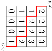 Figure 2
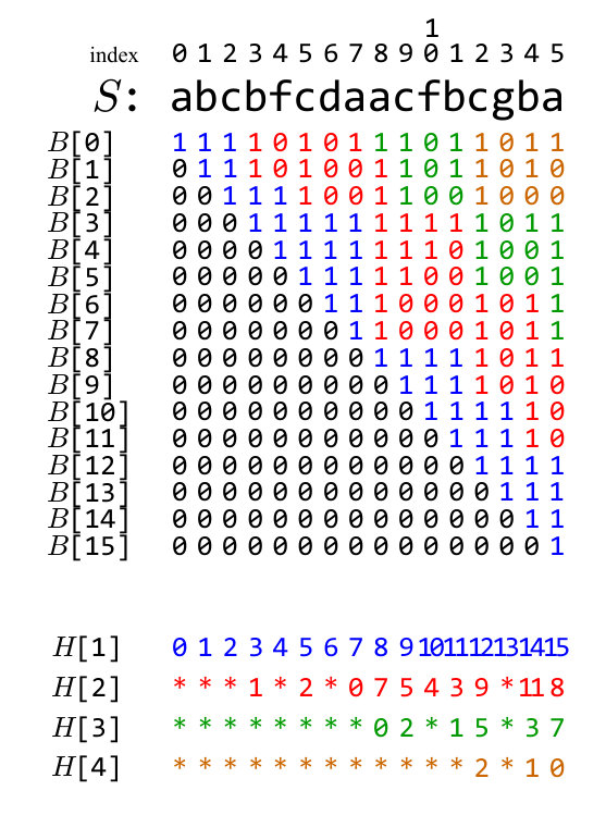 Figure 4
Peer Reviews
No public reviews on file for this paper yet. If you reviewed it on a platform where reviews are public (OpenReview, ICLR, NeurIPS, ICML), you can paste yours below so the community can read it here.
Videos
No videos yet. Explain this paper in a talk, walkthrough, or lecture? Add one.
\Copyright
Sumigawa, Chakraborty, Sadakane and Satti\EventEditorsJohn Q. Open and Joan R. Acces \EventNoEds2 \EventLongTitle42nd Conference on Very Important Topics (CVIT 2016) \EventShortTitleCVIT 2016 \EventAcronymCVIT \EventYear2016 \EventDateDecember 24–27, 2016 \EventLocationLittle Whinging, United Kingdom \EventLogo \SeriesVolume42 \ArticleNo23
Enumerating Range Modes
Kentaro Sumigawa
The University of Tokyo, Japan
Sankardeep Chakraborty
RIKEN Center for Advanced Intelligence Project, Japan
Kunihiko Sadakane
The University of Tokyo, Japan
Srinivasa Rao Satti
Seoul National University, South Korea
Abstract.
We consider the range mode problem where given a sequence and a query range in it, we want to find items with maximum frequency in the range. We give time- and space- efficient algorithms for this problem. Our algorithms are efficient for small maximum frequency cases. We also consider a natural generalization of the problem: the range mode enumeration problem, for which there has been no known efficient algorithms. Our algorithms have query time complexities which is linear to the output size plus small terms.
Key words and phrases:
range mode, space-efficient data structure
1991 Mathematics Subject Classification:
Dummy classification – please refer to http://www.acm.org/about/class/ccs98-html
1. Introduction
We consider the range mode problem, defined as follows.
Definition 1.1** (Mode).**
Given a non-empty multiset , is said to be a mode of , if its multiplicity is no smaller than those of any other elements.
Definition 1.2** (Range mode problem).**
For a sequence and a range of (), output any one of the modes of the multiset .
The problem has many applications in data mining and data analysis [2, 4]. Moreover, there is a strong interest in theory community as well for this problem as it is related to the famous Boolean matrix multiplication and set intersection problem [1].
In this paper, we consider the indexing version of the range mode problem. That is, given a sequence of length , we first construct a data structure, called an index. Then given a query range , we solve the query using the index as well as the input. The algorithm is measured by the index size (in bits) and query time complexity. There are many existing work [8, 1, 9, 6, 3]111The papers [1, 3] have the same title, but some of the results in [3] do not appear in [1]. and some of them are summarized in Table 1.
Our first contribution is space-efficient indexes for the range mode problem, for the case the maximum multiplicity of an item in the set is small. Table 1 summarizes our results. The one in Corollary 3.24 has better time and space complexities than that of [3] with , which is also specialized for small and has space complexity bits and query time complexity .
Our second contribution is efficient indexes for the range mode enumeration problem, defined as follows.
Definition 1.3** (Range Mode Enumeration Problem).**
Given a sequence and a query range , output all items with the largest number of occurrences in the multiset .
Though the problem seems to be a natural generalization of the range mode problem, there has been no existing work. A related and important problem, the set intersection problem [1], has been considered. However, the set intersection problem can be reduced to the range mode enumeration problem, whereas the converse is not true. We cannot use existing algorithms for the set intersection problem to solve the range mode enumeration problem. A simple modification of an existing algorithm [3] works, but it takes time for each output of an item (see Theorem 4.6). We give faster solutions whose query time complexity is linear to the output size plus some small term. Table 2 summarizes the results.
The paper is organized as follows. In Section 2, we review basic properties of the range mode problem and existing algorithms for the range mode problem. We also explain fundamental data structures for storing integer sequences. In Section 3, we give our improved algorithms for the range mode problem. In Section 4, we give algorithms for the range mode enumeration problem. Section 5 summaries the paper. Some of the proofs, algorithms, and figures are given in the appendix.
2. Preliminaries
2.1. Basic properties
To avoid confusion between modes and frequency of modes, from now on we consider range mode problems for not integer sequences but strings on an alphabet. We define the following.
- •
: input string
- •
: the length of string
- •
: the set of characters (alphabet) of
- •
: the frequency of the modes of the substring
- •
: the frequency of a character with maximum frequency, that is,
We assume that there exists a bijection which can be computed in constant time. We sometimes identify characters in the alphabet and integers.
Lemma 2.1**.**
[[7]] If non-empty multisets and a multiset satisfies and if is a mode of , at least one of the following holds.
- •
* is a mode of .*
- •
* belongs to .*
Lemma 2.2**.**
For , if , modes of range are also modes of range .
2.2. Algorithms for the range mode problem
We review the data structure with -word space and query time [3]. The input string of length is partitioned into blocks of length each. In addition to , the data structure has the following four components.
**Two-dimensional array : **
: For each character in the alphabet, an array for storing positions of its occurrences is used.
**Array : **
: For each position of , stores the number of times that the character occurs in the substring .
**Two-dimensional array : **
: The entry of stores the frequency of modes of the substring from the -th block to the -th block. That is, .
**Two-dimensional array : **
: The entry of stores one of the modes of the substring from the -th block to the -th block.
The space complexity is words, for any fixed . Using these arrays, any query is solved in time as follows. If a query is contained inside a block, we scan the range and for each character in the alphabet, we count its number of occurrences. This takes time. If a query range lies on more than one block, we partition the query range into prefix , span , and suffix where . Note that the span may be empty.
From Lemma 2.1, modes of range are either (a) modes of the span, (b) a character in the prefix, or (c) a character in the suffix. For (b) and (c), we scan the prefix and the suffix, and for each character in them, we compute its frequency using the arrays and (for details refer to [3]). For (a), one of the modes of the span and its frequency is obtained from and , respectively. This also takes time.
There exist improved data structures which are summarized in Table 1.
2.3. Representations of integer sequences
We define (increasing monotone sequences) and (decreasing monotone sequences) as follows.
Definition 2.3**.**
*We define as the set of all integer sequences of length such that . We also define as the set of all integer sequences of length such that . *
Theorem 2.4** ([11]).**
For a sequence and an integer , there exists a data structure using bits which can compute
- •
**
- •
**
in time.
Theorem 2.5** (FID [10]).**
For a bit-vector of length which contains ones, consider the following operations.
- •
: returns the -th bit of .
- •
: returns .
- •
: returns .
There exists a data structure which performs the operations in constant time using bits of space.
3. Improved Data Structures for Range Mode Problem
We propose efficient data structures for the range mode problem using , the largest frequency of characters, as a parameter.
Consider the data structure of Section 2.2 with . For simplicity we define for any with . Then the array satisfies the following property.
Property 1**.**
For any adjacent entries in the two-dimensional array , it holds
[TABLE]
From the definition, also satisfies:
Property 2**.**
Any entry of is an integer between and .
Below we propose a data structure for storing in a compressed form and supporting constant time access.
3.1. An efficient representation of the array
We define the set of two-dimensional arrays which have both column-wise and row-wise monotonicity as follows.
Definition 3.1**.**
We define the set of two-dimensional arrays which satisfy all the following inequalities as .
[TABLE]
Theorem 3.2**.**
Let be a two-dimensional array in () and be a non-negative integer. There exists a data structure which can output an entry of in time using bits of space.
Proof 3.3**.**
We prove by induction on that there exists a data structure using at most bits of space, where is some constant satisfying:
- •
There exists a data structure using at most bits of space which can read an entry of in constant time.
Below we show such a constant exists, if we use the data structure of Theorem 2.4.
For , we use the data structure of Theorem 2.4 for storing each column. Then the space usage is at most bits, which is at most bits and the claim holds.
Now we assume that the data structure exists, and prove also exists. We partition the two-dimensional array into blocks where , each of which has columns and rows. The block corresponding to is a two-dimensional array and denoted by . We define flatness of a block as follows.
Definition 3.4**.**
A block is called flat if all the entries in the block are identical.
We also define the height of a block.
Definition 3.5**.**
The height of block , denoted by , is defined as
[TABLE]
That is, the height of a block is the difference between the maximum and the minimum values in the block, plus one.
We prove the following:
Theorem 3.6**.**
Among blocks, there are at most non-flat blocks.
To prove it, we define -th boundary in a block for as follows.
Definition 3.7**.**
For a two-dimensional array , consider the grid graph . The -th boundary of is defined as the edge set of satisfying:
[TABLE]
where we assume .
Then the following holds.
Property 3**.**
The -th boundary is a shortest path from vertex to vertex of the grid graph . That is, if we regard the path as a directed path from to , the edges in the path are of the form of either or .
Example 3.8**.**
Figure 1 shows an array and its second boundary.
Proof 3.9** (Proof of Theorem 3.6).**
It is equivalent that a block is flat, and that any boundary does not pass inside the block. For each of boundaries, the number of blocks in which the boundary passes is . Therefore the number of blocks which contains at least one boundary in it is at most .
Based on this property, we use the following data structure.
**: to store : **
We define . It is clear that .
**: to store differences inside block : **
For non-flat block , we define . Then it holds .
It holds for the original array , , and for flat block , the two-dimensional array is the zero-value array. Then an access to the array is done by Algorithm 1. At line 6 of the algorithm, it is necessary to decide if a block is flat or not. Because a naive data structure using a Boolean array is space-consuming, we develop a space-efficient solution. To do so, we define the following mapping.
Definition 3.10** (Mapping to decide if a block is flat or not).**
*We define a mapping from a block number to a pair of integers as *
[TABLE]
We obtain the following.
Theorem 3.11**.**
For any two distinct non-flat blocks and , it holds .
Proof 3.12**.**
Let and be two distinct non-flat blocks. From the definition of the claim holds if . If , the -th boundary must pass both and . It is however not possible to pass both of them if from Property 3. Thus it holds .
We also define a mapping, which is something like an inverse of .
Definition 3.13**.**
We define a mapping
[TABLE]
as if there exists a non-flat block with , and otherwise.
Then it holds . To use this fact, we have to compute both and . We can compute at line 3 of Algorithm 1 from Definition 3.10. To compute , we use the following.
Lemma 3.14**.**
Assume that . Then if , it holds and .
Finally we obtain:
Theorem 3.15**.**
* is computed in constant time using a data structure of bits.*
Therefore the decision at line 6 of Algorithm 1 is done by using Algorithm 2.
We analyze the space complexity of the data structure .
Lemma 3.16**.**
The size of the data structure is
Next we consider the time to access an entry of . In Algorithm 1, lines 3 and 5 take time. For other lines including the call to Algorithm 2 it takes constant time. Therefore it holds and we obtain .
This completes the proof of Theorem 3.2.
We also obtain:
Theorem 3.17**.**
There exists a data structure of bits supporting an access to in time.
Proof 3.18**.**
We obtain the claim by letting in Theorem 3.2.
By using this data structure for a two-dimensional array satisfying Property 1, we can compute the frequency of the modes of a query range . From Lemma 2.2, a mode is obtained by computing . To compute this, consider the following data structure.
Theorem 3.19**.**
There exists a data structure of bits for given column number of and a value , to compute in constant time.
Proof 3.20**.**
For two-dimensional array , consider the boundaries of Definition 3.7. We can say that is the minimum row number of elements in -th column which are above the -th boundary. Recall that boundaries are shortest paths in the grid graph from vertex to vertex . Consider to encode the boundaries as follows.
Definition 3.21** (A bit-vector representation of a boundary).**
We encode a boundary by a bit-vector of bits as follows. Initially the bit-vector is set empty. We traverse the graph from vertex to vertex along the boundary, and append [math] when we go down, and when we go right, to the end of the bit-vector.
The bit-vector for a boundary has zeros and ones. There are such bit-vectors and the space complexity is bits in total. Let denote the bit-vector for the -th boundary. From definition, it holds . This can be computed in constant time by using FID.
Theorem 3.22**.**
In addition to the string , by using a data structure of bits, we can solve the range mode problem in time.
Proof 3.23**.**
We can use Algorithm 4, where the two-dimensional array satisfies the following:
[TABLE]
By storing the rows or columns in reverse order and subtracting one from all values, belongs to .
In Algorithm 4, the data structures of Theorems 3.2 and 3.19 are used. The space complexity includes bits for Theorem 3.2 and bits for Theorem 3.19, and therefore the total space complexity is bits.
By letting in Theorem 3.22, we obtain:
Corollary 3.24**.**
In addition to the string , using a data structure of bits, the range mode problem is solved in time.
This data structure is superior to the data structure of [3] with , which has space complexity bits and query time complexity , in terms of both time and space.
3.2. Efficient data structure for small
Instead of using the two-dimensional array storing frequencies of all the ranges, we can compute the frequency of modes using only the bit-vector representation of the boundaries of Definition 3.21.
Theorem 3.25**.**
For a two-dimensional array , there exists a data structure of bits that given , to decide if in constant time.
Proof 3.26**.**
We store all the bit-vectors representing the boundaries. It is enough to decide if the -th boundary of is either in the ’s side or ’ size with respect to . This is done by Algorithm 3, which runs in constant time.
From Theorem 3.25, we can compute in time by a binary search on .
Theorem 3.27**.**
There exists a data structure of bits that for a given of , computes the value such that in time.
Proof 3.28**.**
For every column of , we take the set of (at most ) row indexes such that and is a multiple of , and store the set using a predecessor data structure [12]. The space usage for each column is bits, and hence overall bits to represent . The query is supported by finding the predecessor of in the predecessor data structure corresponding to the column .
Now using the structure of Theorem 3.25, we can compute in time by a binary search on , after narrowing down the length of the range of to using the structure of Theorem 3.27. Furthermore, from Theorem 3.19, we can compute an index for modes in constant time. Now we obtain the following theorem.
Theorem 3.29**.**
In addition to the input string , by using a data structure of bits, the range mode problem is solved in time.
Table 1 summarizes the proposed and known data structures.
4. Range Mode Enumeration Problem
Below we consider range modes of a string with alphabet size instead of a sequence . We evaluate algorithms with their space complexity and query time complexity using the size of the output as a parameter.
4.1. Algorithms using existing data structures
Data structures for the range mode problem return only arbitrary one item among all range modes. Instead here we consider a data structure for the problem which returns the leftmost index and the frequency of range modes, where the leftmost index is defined as follows.
Definition 4.1**.**
For a string and query range , the leftmost index of range modes is defined as .
Lemma 4.2**.**
Let be a data structure which returns the leftmost index of range modes for a query range in time using space, there exists a data structure which solves the range mode enumeration problem in time using space.
Proof 4.3**.**
Algorithm 5 solves the problem using the data structure . The algorithm narrows the query range gradually. Because the data structure returns the leftmost index of range modes, the number of range modes for the new query range is exactly one smaller than that of the current query range. Therefore the while loop at line 6 of the algorithm is executed times, and the total time complexity is .
Lemma 4.4**.**
There exists a data structure for finding the leftmost index of range modes and their frequency in time using a data structure with space complexity words in addition to the input string .
Proof 4.5**.**
We slightly change the data structure of [3] described in Section 2.2. Instead of the two-dimensional array storing modes of block ranges, we create another two-dimensional array storing leftmost indices of block ranges. Then we can find the leftmost index of span in constant time. For items appearing in the prefix and the suffix, we can find the leftmost index and its frequency using the same algorithm. Algorithm 6 gives a pseudo code.
From Lemmas 4.2 and 4.4, we obtain the following.
Theorem 4.6**.**
There exists a data structure for the range mode enumeration problem solving a query in time using bits.
4.2. More efficient data structures for enumeration
Definition 4.7**.**
The mode index set for a query range of the range mode enumeration problem is the set of the rightmost position of each mode in the query range. That is,
[TABLE]
Because the set of all range modes can be obtained from the mode index set, below we focus on finding the mode index set.
Define bit-vectors of length each as follows.
[TABLE]
Using these bit-vectors, we obtain:
Theorem 4.8**.**
The set of modes for a query range is .
Proof 4.9**.**
From the definition of , is a mode of range . From Lemma 2.2, is also a mode of range . Conversely, for any index contained in the index set for range , it holds and . Therefore these two sets coincide.
Therefore we can enumerate items in the mode index set by using Algorithm 10.
Consider complexities of the algorithm. For the data structure , which consists of bit-vectors of length , we use bits. We also use bits for the array storing frequencies using bit-vectors, which is used to obtain frequency of modes of a query range. Therefore the total space is bits. As for the time complexity, the algorithm executes Line 7 for times. Lines 3 and 4 takes constant time if we use data structures for bit-vectors. Therefore the total time complexity is . We obtain the following basic data structure.
Theorem 4.10**.**
There exists a data structure for the range mode enumeration problem which computes the mode index set in time using a data structure of bit space in addition to the input string .
Now we improve this using a parameter , the frequency of modes of the entire range. The following lemma holds for the two-dimensional bit-array .
Lemma 4.11**.**
There is the following relation between function and bit-array .
[TABLE]
Proof 4.12**.**
Because , is a mode of range . Using Lemma 2.2, it holds is also a mode of range . From the definition of , we obtain .
Using this property, we define integer sequences of length each.
Definition 4.13**.**
Define integer sequences as follows.
[TABLE]
The bit-array and the sequences have the following relation.
Lemma 4.14**.**
.
Example 4.15**.**
Figure 2 shows an example of bit-array and sequences for string .
Algorithm 10 enumerates indices with bits being set in range of bit-vector . Here for any with , the value of is always . Therefore this operation is identical to enumerate all indices in range of sequence whose value is at least . This problem can be regarded as the range maximum problem.
Definition 4.16** (Range Maximum Problem (RMQ)).**
Given a sequence and query range , the range maximum problem asks an index of the maximum value in the sub-sequence .
Theorem 4.17** ([5]).**
For the range maximum problem of size , there exists a data structure with space complexity bits and query time complexity .
Theorem 4.18**.**
Consider the following problem: Given a sequence , a query range and a threshold , compute . If there exists an oracle to check if it holds for some in constant time, there exists a data structure for the problem with bits and query time.
Consider a data structure to decide if or not for finding the index set. This can be done by using the arrays in Section 2.2 because it is equivalent that and the frequency of in range is at least .
From the observation above, it is enough to use the following data structures to enumerate the solutions.
**Two-dimensional array storing positions of occurrences of symbols: **
An array to store positions of occurrences in ascending order for each symbol of the alphabet
**Array to store ranks for strings: **
An array storing the rank for each index of , that is, stores the number of times that the symbol appears in the substring .
**Two-dimensional array storing frequencies of modes for all ranges: **
The entry of the array stores the frequency of the modes for range .
** bit-vectors storing boundaries of the array : **
The array stores bit-vectors of Definition 3.21.
**Two-dimensional array storing RMQ data structures for arrays of length each: **
An array storing sequences of Definition 4.13 as RMQ data structures. The sequences themselves are not stored.
The space complexity of the two-dimensional array varies depending on which data structure is used. For example, we can use ones in Theorems 3.17 and 3.29. The space complexities of are bits, bits, bits, bits, respectively.
The pseudo code is given in Algorithm 9. Only Line 3 cannot be done in constant time. For other lines, the time complexity is proportional to the number of times the function is executed, and it is .
To recap, the complexities of the algorithms become bit space and query time, where is the space complexity of the two-dimensional array , and is the time complexity to access an entry of . Using Theorems 3.17 and 3.29, we obtain the following.
Theorem 4.19**.**
There exists a data structure with space complexity bits in addition to the input string , which solves a query in time .
Theorem 4.20**.**
There exists a data structure with space complexity bits in addition to the input string , which solves a query in time .
By combining the data structure of [3], we can further reduce the space complexity. Consider a string which stores symbols of whose frequencies are at least , and a string which stores the rest of the symbols. The string stores at most distinct symbols. Using the data structures of [3] and Theorem 4.20 for and respectively, the following holds.
Theorem 4.21**.**
There exists a data structure with space complexity bits in addition to the input string , which solves a query in time .
The proposed data structures for the range mode enumeration problem are summarized in Table 2.
5. Concluding Remarks
In this paper, we have given more efficient algorithms for the indexing version of the range mode problem. Our algorithms are more space- and time- efficient for small maximum frequency case than existing ones. We have also considered a natural extension of the range mode problem: range mode enumeration problem and given fast algorithms.
There are other related problems like Boolean matrix multiplication problem. A future work, we will give efficient algorithms for these problems.
Appendix A Omitted Proofs
A.1. Proof of Lemma 2.1
Proof A.1**.**
We prove by contradiction. Let be a mode of , and assume is not a mode of and . Let be a mode of . From the definition the multiplicity of in is strictly larger than that of in . Because , the multiplicity of in is equal to that of in , and it is smaller than that of in . This contradicts that is a mode of .
A.2. Proof of Lemma 2.2
Proof A.2**.**
Let be any mode in range and be its frequency. Because range contains range , the frequency of in range is at least . On the other hand, because , the frequency of in range is at most . Therefore the frequency of in range becomes and is also a mode in range .
A.3. Proof of Lemma 3.16
If , the space complexity of the two-dimensional array is, from the assumption of ,
[TABLE]
If , it can be stored in bits by using the data structure for each row. Therefore for any case can be stored in at most bits.
Next we consider the space complexity of storing differences inside non-flat blocks.
Lemma A.3**.**
For the summation of all , it holds .
Proof A.4**.**
From the column-wise and row-wise monotonicity, for each , it holds . By summing this for all , we obtain the claim.
Consider the space complexity of the data structure storing for non-flat blocks . If , by using , the space becomes bits. If , we store each row of the two-dimensional array in bits by using which support constant access. For both time and space, the former case has worse complexities. Therefore we analyze the space by assuming every block is stored in bits.
[TABLE]
We also need to store pointers to the data structures because their size varies depending on . As a bijection between and , we define . By using this, we can regard the pointers to the data structures as a monotone increasing sequence with terms and range . By representing by the data structure , it holds
[TABLE]
Therefore the space is upper-bounded by bits.
The total space of the data structures for is:
[TABLE]
By letting , for any positive integer , it holds
[TABLE]
This proves there exists a data structure of bits for .
A.4. Proof of Theorem 3.15
Proof A.5**.**
We use a two-dimensional Boolean array of bits storing for each member of , True if and False if . In addition to this, for each we create two integer sequences of length each, as follows. For each , we define if . If , we choose arbitrary values for and satisfying . From Lemma 3.14, such sequences must exist. By using the data structure we can store each sequence in at most bits and access in constant time. The total space for these sequences is at most bits.
A.5. Proof of Theorem 4.18
Proof A.6**.**
We recursively find range maximum values as in Algorithm 7. Consider the number of times that the function of Algorithm 8 is called. The number of times that an item is added to the set in the function is at most . On the other hand, if , the number of times that any item is not added to the set is at most , for ranges . Therefore the total number of times that is called is at most . From the assumption of the oracle, Algorithm 7 runs in time. Because the algorithm uses no data structures other than RMQ, the space complexity is bits.
Appendix B Omitted Pseudo codes and Figures
The reference list from the paper itself. Each links out to its DOI / PubMed record.
- 1[1] Timothy M. Chan, Stephane Durocher, Kasper Green Larsen, Jason Morrison, and Bryan T. Wilkinson. Linear-space data structures for range mode query in arrays. Theory of Computing Systems , 55(4):719–741, Nov 2014. doi:10.1007/s 00224-013-9455-2 . · doi ↗
- 2[2] Erik D. Demaine, Alejandro López-Ortiz, and J. Ian Munro. Frequency estimation of internet packet streams with limited space. In Algorithms - ESA 2002, 10th Annual European Symposium, Rome, Italy, September 17-21, 2002, Proceedings , pages 348–360, 2002.
- 3[3] Stephane Durocher and Jason Morrison. Linear-space data structures for range mode query in arrays. Co RR , abs/1101.4068, 2011. ar Xiv:1101.4068 .
- 4[4] Min Fang, Narayanan Shivakumar, Hector Garcia-Molina, Rajeev Motwani, and Jeffrey D. Ullman. Computing iceberg queries efficiently. In VLDB’98, Proceedings of 24rd International Conference on Very Large Data Bases, August 24-27, 1998, New York City, New York, USA , pages 299–310, 1998. URL: http://www.vldb.org/conf/1998/p 299.pdf .
- 5[5] J. Fischer and V. Heun. Space-Efficient Preprocessing Schemes for Range Minimum Queries on Static Arrays. SIAM Journal on Computing , 40(2):465–492, 2011.
- 6[6] Mark Greve, Allan Grønlund Jørgensen, Kasper Dalgaard Larsen, and Jakob Truelsen. Cell probe lower bounds and approximations for range mode. In Automata, Languages and Programming, 37th International Colloquium, ICALP 2010, Bordeaux, France, July 6-10, 2010, Proceedings, Part I , pages 605–616, 2010.
- 7[7] Danny Krizanc, Pat Morin, and Michiel Smid. Range mode and range median queries on lists and trees. Nordic J. of Computing , 12(1):1–17, March 2005. URL: http://dl.acm.org/citation.cfm?id=1195881.1195882 .
- 8[8] Holger Petersen. Improved bounds for range mode and range median queries. In Viliam Geffert, Juhani Karhumäki, Alberto Bertoni, Bart Preneel, Pavol Návrat, and Mária Bieliková, editors, SOFSEM 2008: Theory and Practice of Computer Science , pages 418–423, Berlin, Heidelberg, 2008. Springer Berlin Heidelberg.