First-order optimization algorithms via inertial systems with Hessian driven damping
Hedy Attouch, Zaki Chbani, Jalal Fadili, Hassan Riahi

TL;DR
This paper introduces new first-order optimization algorithms inspired by inertial systems with Hessian-driven damping, achieving rapid convergence and extending to non-smooth convex functions with acceleration techniques.
Contribution
The paper develops novel first-order algorithms based on inertial dynamics with Hessian-driven damping, extending them to non-smooth functions and incorporating acceleration via time scale factors.
Findings
Algorithms exhibit rapid convergence towards zero gradients.
Extension to non-smooth convex functions using Moreau envelope.
Numerical results support theoretical convergence claims.
Abstract
In a Hilbert space setting, for convex optimization, we analyze the convergence rate of a class of first-order algorithms involving inertial features. They can be interpreted as discrete time versions of inertial dynamics involving both viscous and Hessian-driven dampings. The geometrical damping driven by the Hessian intervenes in the dynamics in the form . By treating this term as the time derivative of , this gives, in discretized form, first-order algorithms in time and space. In addition to the convergence properties attached to Nesterov-type accelerated gradient methods, the algorithms thus obtained are new and show a rapid convergence towards zero of the gradients. On the basis of a regularization technique using the Moreau envelope, we extend these methods to non-smooth convex functions with extended real values. The…
Click any figure to enlarge with its caption.
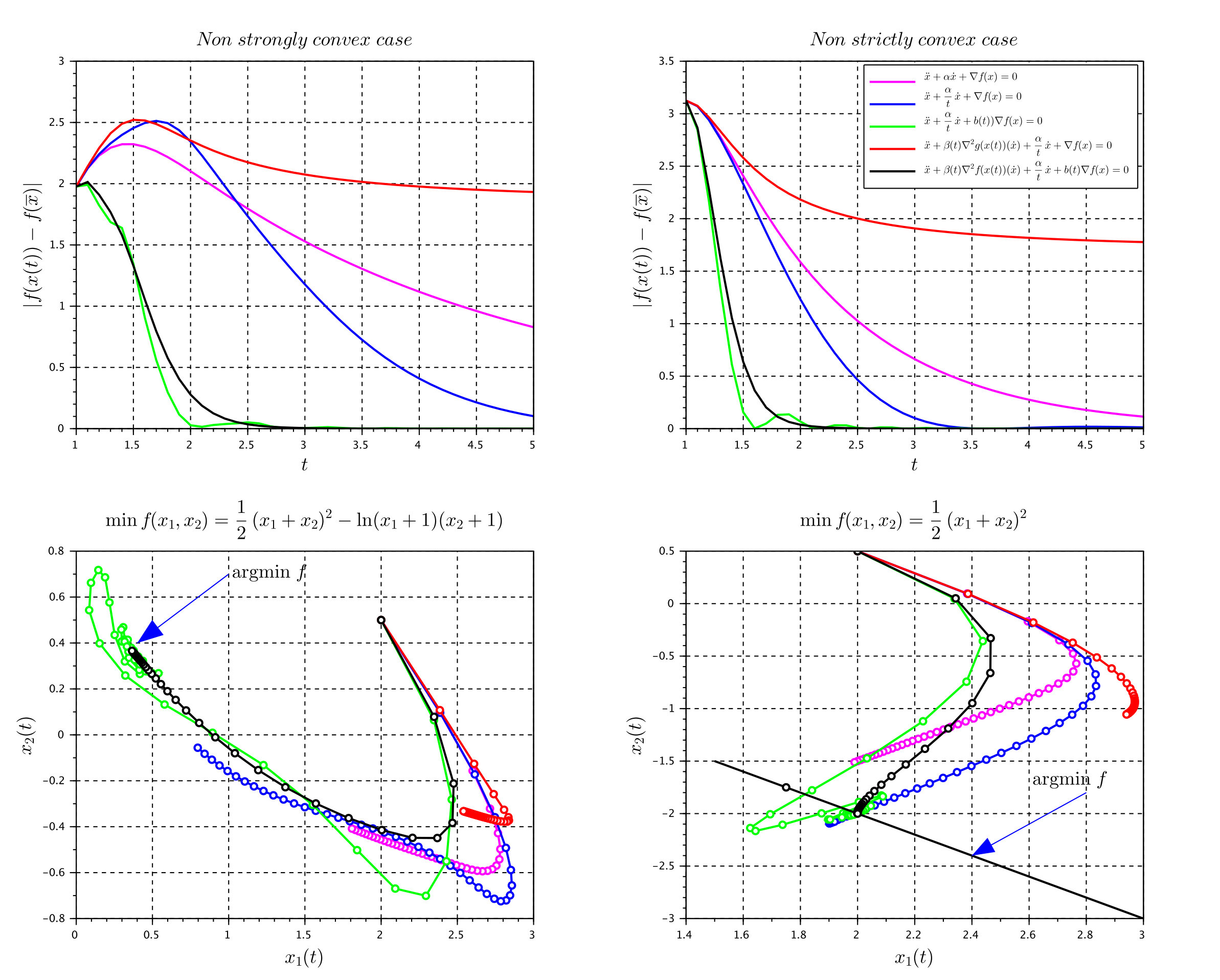 Figure 1
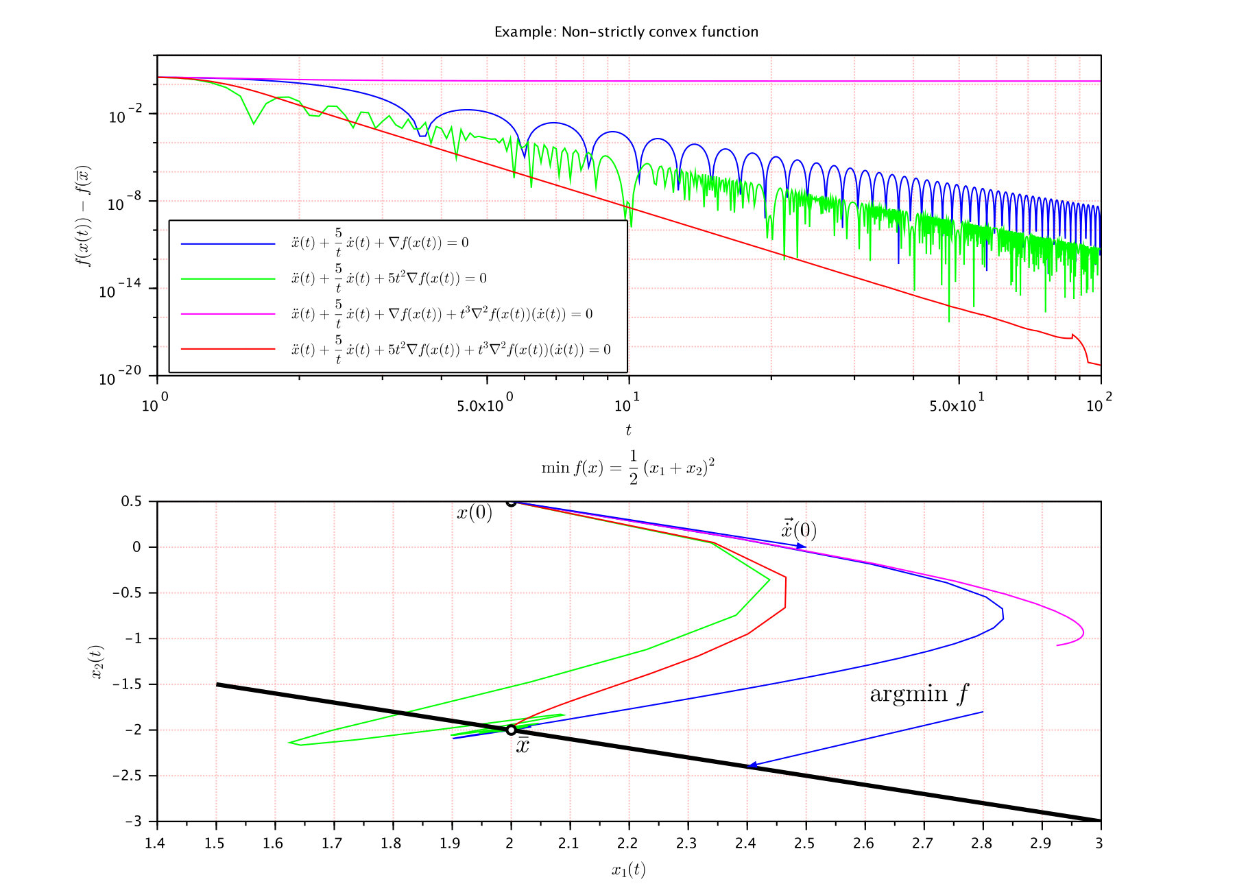 Figure 2
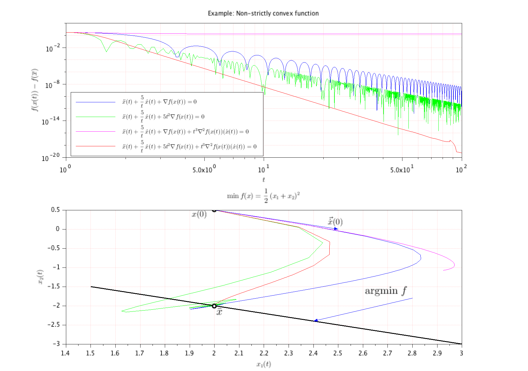 Figure 3
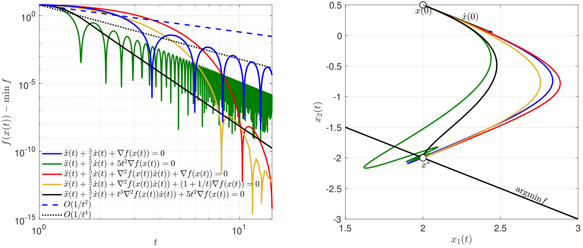 Figure 4
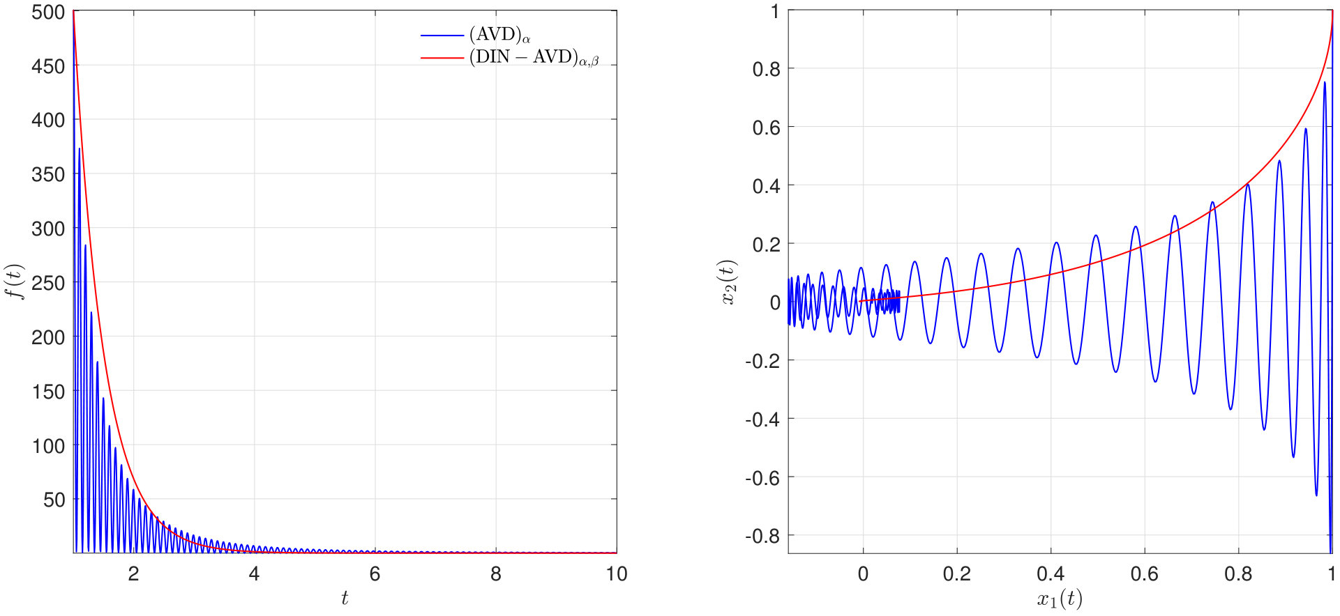 Figure 5
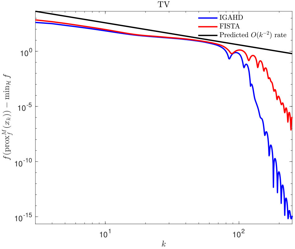 Figure 6
 Figure 7
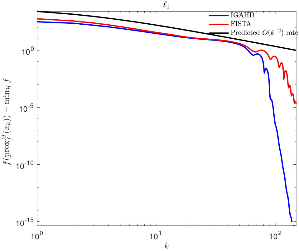 Figure 8
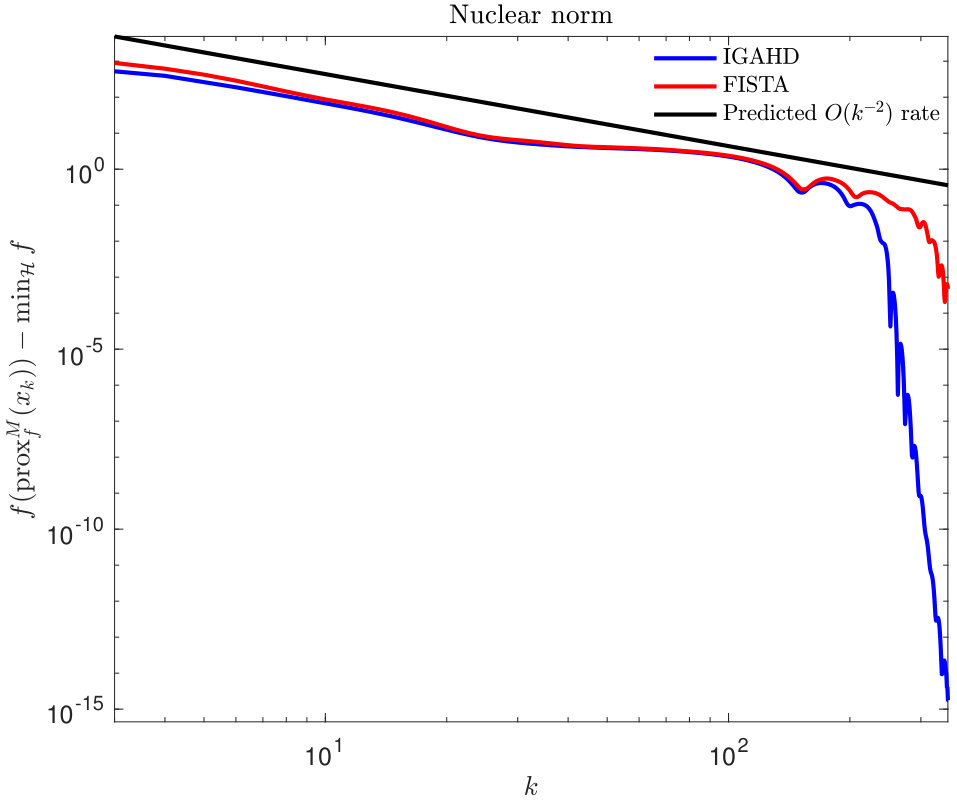 Figure 9
Peer Reviews
No public reviews on file for this paper yet. If you reviewed it on a platform where reviews are public (OpenReview, ICLR, NeurIPS, ICML), you can paste yours below so the community can read it here.
Videos
No videos yet. Explain this paper in a talk, walkthrough, or lecture? Add one.
∎
11institutetext: H. Attouch 22institutetext: IMAG, Univ. Montpellier, CNRS, Montpellier, France
22email: [email protected] 33institutetext: Z. Chbani 44institutetext: Cadi Ayyad Univ., Faculty of Sciences Semlalia, Mathematics, 40000 Marrakech, Morroco
44email: [email protected] 55institutetext: J. Fadili 66institutetext: GREYC CNRS UMR 6072, Ecole Nationale Supérieure d’Ingénieurs de Caen, France
66email: [email protected] 77institutetext: H. Riahi 88institutetext: Cadi Ayyad Univ., Faculty of Sciences Semlalia, Mathematics, 40000 Marrakech, Morroco 88email: [email protected]
First-order optimization algorithms via inertial systems with Hessian driven damping
Hedy Attouch
Zaki Chbani
Jalal Fadili
Hassan Riahi
(July 19, 2019)
Abstract
In a Hilbert space setting, for convex optimization, we analyze the convergence rate of a class of first-order algorithms involving inertial features. They can be interpreted as discrete time versions of inertial dynamics involving both viscous and Hessian-driven dampings. The geometrical damping driven by the Hessian intervenes in the dynamics in the form . By treating this term as the time derivative of , this gives, in discretized form, first-order algorithms in time and space. In addition to the convergence properties attached to Nesterov-type accelerated gradient methods, the algorithms thus obtained are new and show a rapid convergence towards zero of the gradients. On the basis of a regularization technique using the Moreau envelope, we extend these methods to non-smooth convex functions with extended real values. The introduction of time scale factors makes it possible to further accelerate these algorithms. We also report numerical results on structured problems to support our theoretical findings.
Keywords:
Hessian driven damping; inertial optimization algorithms; Nesterov accelerated gradient method; Ravine method; time rescaling.
††journal: Math. Program. Ser. A
AMS subject classification
37N40, 46N10, 49M30, 65B99, 65K05, 65K10, 90B50, 90C25.
1 Introduction
Unless specified, throughout the paper we make the following assumptions
[TABLE]
As a guide in our study, we will rely on the asymptotic behavior, when , of the trajectories of the inertial system with Hessian-driven damping
[TABLE]
and are damping parameters, and is a time scale parameter.
The time discretization of this system will provide a rich family of first-order methods for minimizing . At first glance, the presence of the Hessian may seem to entail numerical difficulties. However, this is not the case as the Hessian intervenes in the above ODE in the form , which is nothing but the derivative w.r.t. time of . This explains why the time discretization of this dynamic provides first-order algorithms. Thus, the Nesterov extrapolation scheme Nest1 ; Nest4 is modified by the introduction of the difference of the gradients at consecutive iterates. This gives algorithms of the form
[TABLE]
where , to be specified later, is an operator involving the gradient or the proximal operator of .
Coming back to the continuous dynamic, we will pay particular attention to the following two cases, specifically adapted to the properties of :
For a general convex function , taking , gives
[TABLE]
In the case , , , it can be interpreted as a continuous version of the Nesterov accelerated gradient method SBC . According to this, in this case, we will obtain convergence rates for the objective values. 2.
For a -strongly convex function , we will rely on the autonomous inertial system with Hessian driven damping
[TABLE]
and show exponential (linear) convergence rate for both objective values and gradients.
For an appropriate setting of the parameters, the time discretization of these dynamics provides first-order algorithms with fast convergence properties. Notably, we will show a rapid convergence towards zero of the gradients.
1.1 A historical perspective
B. Polyak initiated the use of inertial dynamics to accelerate the gradient method in optimization. In Pol ; Polyak2 , based on the inertial system with a fixed viscous damping coefficient
[TABLE]
he introduced the Heavy Ball with Friction method. For a strongly convex function , (HBF) provides convergence at exponential rate of to . For general convex functions, the asymptotic convergence rate of (HBF) is (in the worst case). This is however not better than the steepest descent. A decisive step to improve (HBF) was taken by Alvarez-Attouch-Bolte-Redont AABR by introducing the Hessian-driven damping term , that is (DIN)0,β . The next important step was accomplished by Su-Boyd-Candès SBC with the introduction of a vanishing viscous damping coefficient , that is (AVD)α (see Section 1.1.2). The system (DIN-AVD)α,β,1 (see Section 2) has emerged as a combination of (DIN)0,β and (AVD)α . Let us review some basic facts concerning these systems.
1.1.1 The (DIN)γ,β dynamic
The inertial system
[TABLE]
was introduced in AABR . In line with (HBF), it contains a fixed positive friction coefficient . The introduction of the Hessian-driven damping makes it possible to neutralize the transversal oscillations likely to occur with (HBF), as observed in AABR in the case of the Rosenbrook function. The need to take a geometric damping adapted to had already been observed by Alvarez Alv0 who considered
[TABLE]
where is a linear positive anisotropic operator. But still this damping operator is fixed. For a general convex function, the Hessian-driven damping in (DIN)γ,β performs a similar operation in a closed-loop adaptive way. The terminology (DIN) stands shortly for Dynamical Inertial Newton. It refers to the natural link between this dynamic and the continuous Newton method.
1.1.2 The (AVD)α dynamic
The inertial system
[TABLE]
was introduced in the context of convex optimization in SBC . For general convex functions it provides a continuous version of the accelerated gradient method of Nesterov. For , each trajectory of (AVD)α satisfies the asymptotic rate of convergence of the values . As a specific feature, the viscous damping coefficient vanishes (tends to zero) as time goes to infinity, hence the terminology. The convergence properties of the dynamic (AVD)α have been the subject of many recent studies, see AAD ; AC1 ; AC2 ; AC2R-EECT ; ACPR ; ACR-subcrit ; AP ; AD ; AD17 ; May ; SBC . They helped to explain why is a wise choise of the damping coefficient.
In CEG1 , the authors showed that a vanishing damping coefficient dissipates the energy, and hence makes the dynamic interesting for optimization, as long as . The damping coefficient can go to zero asymptotically but not too fast. The smallest which is admissible is of order . It enforces the inertial effect with respect to the friction effect.
The tuning of the parameter in front of comes from the Lyapunov analysis and the optimality of the convergence rates obtained. The case , which corresponds to Nesterov’s historical algorithm, is critical. In the case , the question of the convergence of the trajectories remains an open problem (except in one dimension where convergence holds ACR-subcrit ). As a remarkable property, for , it has been shown by Attouch-Chbani-Peypouquet-Redont ACPR that each trajectory converges weakly to a minimizer. The corresponding algorithmic result has been obtained by Chambolle-Dossal CD . For , it is shown in AP and May that the asymptotic convergence rate of the values is actually . The subcritical case has been examined by Apidopoulos-Aujol-DossalAAD and Attouch-Chbani-Riahi ACR-subcrit , with the convergence rate of the objective values . These rates are optimal, that is, they can be reached, or approached arbitrarily close:
: the optimal rate is achieved by taking with ( become very flat around its minimum), see ACPR .
: the optimal rate is achieved by taking , see AAD .
The inertial system with a general damping coefficient was recently studied by Attouch-Cabot in AC1 ; AC2 , and Attouch-Cabot-Chbani-Riahi in AC2R-EECT .
1.1.3 The (DIN-AVD)α,β dynamic
The inertial system
[TABLE]
was introduced in APR . It combines the two types of damping considered above. Its formulation looks at a first glance more complicated than (AVD)α . In APR2 , Attouch-Peypouquet-Redont showed that (DIN-AVD)α,β is equivalent to the first-order system in time and space
[TABLE]
This provides a natural extension to proper lower semicontinuous and convex, just replacing the gradient by the subdifferential.
To get better insight, let us compare the two dynamics (AVD)α and (DIN-AVD)α,β on a simple quadratic minimization problem, in which case the trajectories can be computed in closed form as explained in Appendix A.3. Take and , which is ill-conditioned. We take parameters , , so as to obey the condition . Starting with initial conditions: , , we have the trajectories displayed in Figure 1. This illustrates the typical situation of an ill-conditioned minimization problem, where the wild oscillations of (AVD)α are neutralized by the Hessian damping in (DIN-AVD)α,β (see Appendix A.3 for further details).
1.2 Main algorithmic results
Let us describe our main convergence rates for the gradient type algorithms. Corresponding results for the proximal algorithms are also obtained.
General convex function
Let be a convex function whose gradient is -Lipschitz continuous. Based on the discretization of (DIN-AVD) , we consider
[TABLE]
Suppose that , , . In Theorem 3.3, we show that
[TABLE]
Strongly convex function
When is -strongly convex for some , our analysis relies on the autonomous dynamic with . Based on its time discretization, we obtain linear convergence results for the values (hence the trajectory) and the gradients terms. Explicit discretization gives the inertial gradient algorithm
[TABLE]
Assuming that is -Lipschitz continuous, sufficiently small and , it is shown in Theorem 5.3 that, with ( )
[TABLE]
Moreover, the gradients converge exponentially fast to zero.
1.3 Contents
The paper is organized as follows. Sections 2 and 3 deal with the case of general convex functions, respectively in the continuous case and the algorithmic cases. We improve the Nesterov convergence rates by showing in addition fast convergence of the gradients. Sections 4 and 5 deal with the same questions in the case of strongly convex functions, in which case, linear convergence results are obtained. Section 6 is devoted to numerical illustrations. We conclude with some perspectives.
2 Inertial dynamics for general convex functions
Our analysis deals with the inertial system with Hessian-driven damping
[TABLE]
2.1 Convergence rates
We start by stating a fairly general theorem on the convergence rates and integrability properties of (DIN-AVD)α,β,b under appropriate conditions on the parameter functions and . As we will discuss shortly, it turns out that for some specific choices of the parameters, one can recover most of the related results existing in the literature. The following quantities play a central role in our analysis:
[TABLE]
Theorem 2.1
Consider (DIN-AVD)α,β,b , where () holds. Take . Let be a solution trajectory of (DIN-AVD)α,β,b . Suppose that the following growth conditions are satisfied:
[TABLE]
Then, is positive and
[TABLE]
Proof
Given , define for
[TABLE]
where
The function will serve as a Lyapunov function. Differentiating gives
[TABLE]
Using equation (DIN-AVD)α,β,b , we have
[TABLE]
Hence,
[TABLE]
Let us go back to (3). According to the choice of , the terms cancel, which gives
[TABLE]
Condition gives . Combining this equation with convexity of ,
[TABLE]
we obtain the inequality
[TABLE]
Then note that
[TABLE]
Hence, condition writes equivalently
[TABLE]
which, by (4), gives . Therefore, is non-increasing, and hence . Since all the terms that enter are nonnegative, we obtain . Then, by integrating (4) we get
[TABLE]
and
[TABLE]
which gives and , and completes the proof. ∎
2.2 Particular cases
As anticipated above, by specializing the functions and , we recover most known results in the literature; see hereafter for each specific case and related literature. For all these cases, we will argue also on the interest of our generalization.
Case 1
The (DIN-AVD)α,β system corresponds to and . In this case, . Conditions and are satisfied by taking and . Hence, as a consequence of Theorem 2.1, we obtain the following result of Attouch-Peypouquet-Redont APR2 :
Theorem 2.2 (APR2 )
Let be a trajectory of the dynamical system (DIN-AVD)α,β . Suppose . Then
[TABLE]
Case 2
The system(DIN-AVD) , which corresponds to and , was considered in SDJS . Compared to (DIN-AVD)α,β it has the additional coefficient in front of the gradient term. This vanishing coefficient will facilitate the computational aspects while keeping the structure of the dynamic. Observe that in this case, . Conditions and boil down to . Hence, as a consequence of Theorem 2.1, we obtain
Theorem 2.3
Let be a solution trajectory of the dynamical system (DIN-AVD) . Suppose . Then
[TABLE]
Case 3
The dynamical system (DIN-AVD)α,0,b , which corresponds to , was considered by Attouch-Chbani-Riahi in ACR-rescale . It comes also naturally from the time scaling of (AVD)α . In this case, we have . Condition is equivalent to . becomes
[TABLE]
which is precisely the condition introduced in (ACR-rescale, , Theorem 8.1). Under this condition, we have the convergence rate
[TABLE]
This makes clear the acceleration effect due to the time scaling. For , we have , under the assumption .
Case 4
Let us illustrate our results in the case , . We have The conditions can be written respectively as:
[TABLE]
When , the conditions (7) are equivalent to which gives the convergence rate .
Let us apply these choices to the quadratic function . is convex but not strongly so, and . The closed-form solution of the ODE with this choice of and is given in Appendix A.3. We choose the values and in order to satisfy condition (7). The left panel of Figure 2 depicts the convergence profile of the function value, and its right panel the trajectories associated with the system (DIN-AVD)α,β,b for different scenarios of the parameters. Once again, the damping of oscillations due to the presence of the Hessian is observed.
Discussion
Let us first apply the above choices of for each case to the quadratic function . is convex but not strongly so, and . The closed-form solution of (DIN-AVD)α,β,b with each choice of and is given in Appendix A.3. For all cases, we set . For case 1, we set . For case 2, we take . As for case 3, we set . For case 4, we choose and in order to satisfy condition (7). The left panel of Figure 2 depicts the convergence profile of the function value as well as the predicted convergence rates and (the latter is for cases with time (re)scaling). The right panel of Figure 2 displays the associated trajectories for the different scenarios of the parameters.
The rates one can achieve in our Theorem 2.1 look similar to those in Theorem 2.2 and Theorem 2.3. Thus one may wonder whether our framework allowing for more general variable parameters is necessary. The answer is affirmative for several reasons. First, our framework can be seen as a one-stop shop allowing for a unified analysis with an unprecedented level of generality. It also handles time (re)scaling straightforwardly by appropriately setting the functions and (see Case 3 and 4 above). In addition, though these convergence rates appear similar, one has to keep in mind that these are upper-bounds. It turns out from our detailed example in the quadratic case introduced above in Figure 2, that not only the oscillations are reduced due to the presence of Hessian damping, but also the trajectory and the objective can be made much less oscillatory thanks to the flexible choice of the parameters allowed by our framework. This is yet again another evidence of the interest of our setting.
3 Inertial algorithms for general convex functions
3.1 Proximal algorithms
3.1.1 Smooth case
Writing the term in (DIN-AVD)α,β,b as the time derivative of , and taking the implicit time discretization of this system, with step size , gives
[TABLE]
Equivalently
[TABLE]
Observe that this requires to be only of class . Set now . We obtain the following algorithm with and varying with :
[TABLE]
Theorem 3.1
Assume that is a convex function. Suppose that . Set
[TABLE]
and suppose that the following growth conditions are satisfied:
[TABLE]
Then, is positive and, for any sequence generated by
[TABLE]
Before delving into the proof, the following remarks on the choice/growth of the parameters are in order.
Remark 1
We first observe that condition is nothing but a forward (explicit) discretization of its continuous analogue . In addition, in view of (1), equivalently reads
[TABLE]
In turn, (10) and are explicit discretizations of (1) and respectively.
Remark 2
The convergence rate on the objective values in Theorem 3.1(i) is with the proviso that
[TABLE]
which in turn implies . If, in addition to (11), we also have , then the summability property in Theorem 3.1(ii) reads . For instance, if is non-increasing and , , then (11) is in force with as a lower-bound on the infimum. In summary, we get under fairly general assumptions on the growth of the sequences and .
Let us now exemplify choices of and that have the appropriate growth as above and comply with (11) (hence ) as well as .
Let us take and , which is the discrete analogue of the continuous case 1 considered in Section 2.2 (recall that the continuous version was analyzed in APR2 ). Note however that APR2 did not study the discrete (algorithmic) case and thus our result is new even for this system. In such a case, and is obviously non-icnreasing. Thus, if , then one easily checks that (11) (hence ) and are in force for all . 2.
Consider now the discrete counterpart of case 2 in Section 2.2. Take and 111One can even consider the more general case for which our discussion remains true under minor modifications. But we do not pursue this for the sake of simplicity.. Thus . This case was studied in SDJS both in the continuous setting and for the gradient algorithm, but not for the proximal algorithm. This choice is a special case of the one discussed above since is the constant sequence and . Thus (11) (hence ) holds. is also verified for all as soon as .
Proof
Given , set
[TABLE]
where
[TABLE]
and is a positive sequence that will be adjusted. Observe that is nothing but the discrete analogue of the Lyapunov function (2). Set , i.e.,
[TABLE]
Let us evaluate the last term of the above expression with the help of the three-point identity
Using successively the definition of and (8), we get
[TABLE]
Set shortly . We have obtained
[TABLE]
By virtue of , we have
[TABLE]
Then, in the above expression, the coefficient of is less or equal than zero, which gives
[TABLE]
According to the (convex) subdifferential inequality and (by ), we infer
[TABLE]
Take \delta_{k}:=-hC_{k}(k+1)=h\Big{(}b_{k}hk-\beta_{k+1}-k(\beta_{k+1}-\beta_{k})\Big{)}(k+1) so that the terms cancel in . We obtain
[TABLE]
Equivalently
[TABLE]
By assumption , we have . Therefore, the sequence is non-increasing, which, by definition of , gives, for
[TABLE]
By summing the inequalities
[TABLE]
we finally obtain ∎
3.1.2 Non-smooth case
Let be a proper lower semicontinuous and convex function. We rely on the basic properties of the Moreau-Yosida regularization. Let be the Moreau envelope of of index , which is defined by:
[TABLE]
We recall that is a convex function, whose gradient is -Lipschitz continuous, such that . The interested reader may refer to BC ; Bre1 for a comprehensive treatment of the Moreau envelope in a Hilbert setting. Since the set of minimizers is preserved by taking the Moreau envelope, the idea is to replace by in the previous algorithm, and take advantage of the fact that is continuously differentiable. The Hessian dynamic attached to becomes
[TABLE]
However, we do not really need to work on this system (which requires to be ), but with the discretized form which only requires the function to be continuously differentiable, as is the case of . Then, algorithm applied to now reads
[TABLE]
By applying Theorem 3.1 we obtain that under the assumption and ,
Thus, we just need to formulate these results in terms of and its proximal mapping. This is straightforward thanks to the following formulae from proximal calculus BC :
[TABLE]
We obtain the following relaxed inertial proximal algorithm (NS stands for Non-Smooth):
[TABLE]
Theorem 3.2
Let be a convex, lower semicontinuous, proper function. Let the sequence as defined in (10), and suppose that the growth conditions and in Theorem 3.1 are satisfied. Then, for any sequence generated by (IPAHD-NS) , the following holds
[TABLE]
3.2 Gradient algorithms
Take a convex function whose gradient is -Lipschitz continuous. Our analysis is based on the dynamic (DIN-AVD) considered in Theorem 2.3 with damping parameters , . Consider the time discretization of (DIN-AVD)
[TABLE]
with inspired by Nesterov’s accelerated scheme. We obtain the following scheme:
[TABLE]
Following AC2 , set , whence .
Given , our Lyapunov analysis is based on the sequence
[TABLE]
Theorem 3.3
Let be a convex function whose gradient is -Lipschitz continuous. Let be a sequence generated by algorithm (IGAHD) , where , and . Then the sequence defined by (17)-(18) is non-increasing, and the following convergence rates are satisfied:
[TABLE]
Proof
We rely on the following reinforced version of the gradient descent lemma (Lemma 1 in Appendix A.1). Since , and is -Lipschitz continuous,
[TABLE]
for all . Let us write it successively at and , then at , . According to and , we get
[TABLE]
Multiplying (19) by , then adding (20), we derive that
[TABLE]
Let us multiply (3.2) by to make appear . We obtain
[TABLE]
Since we have , which gives
[TABLE]
According to the definition of , we infer
[TABLE]
Let us compute this last expression with the help of the elementary identity
[TABLE]
By definition of , according to (IGAHD) and , we have
[TABLE]
Hence
[TABLE]
Collecting the above results, we obtain
[TABLE]
Equivalently
[TABLE]
with
[TABLE]
Consequently
[TABLE]
where
[TABLE]
When we have . Let us analyze the sign of in the case . Set , . We have
[TABLE]
Elementary algebra gives that the above quadratic form is non-negative when
[TABLE]
Recall that is of order . Hence, this inequality is satisfied for large enough if , which is equivalent to Under this condition , which gives conclusion . Similar argument gives that for (such exists according to assumption )
[TABLE]
After summation of these inequalities, we obtain conclusion . ∎
Remark 3
In (WRJ, , Theorem 8), the same convergence rate as in Theorem 3.3 on the objective values is obtained for a very different discretization of the system (DIN-AVD) . Their scheme is thus related but quite different from (IGAHD) . Their claims require also intricate conditions relating to hold true.
In Theorem 3.3, the condition essentially reveals that in order to preserve acceleration offered by the viscous damping, the geometric damping should not be too large. It is an open question whether this constraint is a technical artifact or is fundamental to acceleration. We leave it to a future work.
Remark 4
From we immediately infer that for
[TABLE]
A similar argument holds for . Hence
[TABLE]
Remark 5
In Theorem 3.3, the convergence property of the values is expressed according to the sequence . It is natural to know if a similar result is true for the sequence . This is an open question in the case of Nesterov’s accelerated gradient method and the corresponding FISTA algorithm for structured minimization Nest4 ; BT . In the case of the Hessian-driven damping algorithms, we give a partial answer to this question. By the classical descent lemma, and the monotonicity of we have
[TABLE]
According to we obtain
[TABLE]
From Theorem 3.3 we deduce that
[TABLE]
Remark 6
When is a proper lower semicontinuous proper function, but not necessarily smooth, we follow the same reasoning as in Section 3.1.2. We consider minimizing the Moreau envelope of , whose gradient is -Lipschitz continuous, and then apply (IGAHD) to . We omit the details for the sake of brevity. This observation will be very useful to solve even structured composite problems as we will describe in Section 6.
4 Inertial dynamics for strongly convex functions
4.1 Smooth case
Recall the classical definition of strong convexity:
Definition 1
A function is said to be -strongly convex for some if is convex.
For strongly convex functions, a suitable choice of and in (DIN)γ,β provides exponential decay of the value function (hence of the trajectory), and of the gradients.
Theorem 4.1
Suppose that () holds where is in addition -strongly convex for some . Let be a solution trajectory of
[TABLE]
Suppose that . Then, the following hold:
- (i)
for all
[TABLE]
where C:=f(x(t_{0}))-\min_{{\mathcal{H}}}f+\mu{\color[rgb]{0,0,0}{\|x(t_{0})-x^{\star}\|^{2}}}+\|\dot{x}(t_{0})+\beta\nabla f(x(t_{0}))\|^{2}. 2. (ii)
There exists some constant such that, for all
[TABLE]
Moreover,
When , we have
Remark 7
When , Theorem 4.1 recovers (Siegel, , Theorem 2.2). In the case , a result on a related but different dynamical system can be found in (WRJ, , Theorem 1) (their rate is also sligthtly worse than ours). Our gradient estimate is distinctly new in the literature.
Proof
- (i)
Let be the unique minimizer of . Define by
[TABLE]
Set . Derivation of gives
[TABLE]
Using (22), we get
[TABLE]
After developing and simplification, we obtain
[TABLE]
By strong convexity of we have
[TABLE]
Thus, combining the last two relations we obtain
[TABLE]
where (the variable is omitted to lighten the notation)
[TABLE]
Let us formulate with .
[TABLE]
After developing and simplifying, we obtain
[TABLE]
Since , we immediately get Hence
[TABLE]
Let us use again the strong convexity of to write
[TABLE]
By combining the two inequalities above, we obtain
[TABLE]
where .
Set , . Elementary algebraic computation gives that, under the condition
[TABLE]
Hence for
[TABLE]
By integrating the differential inequality above we obtain
[TABLE]
By definition of , we infer
[TABLE]
and
[TABLE] 2. (ii)
Set . Developing the above expression, we obtain
[TABLE]
By convexity of we have . Moreover,
[TABLE]
Combining the above results, we obtain
[TABLE]
Set . We have
[TABLE]
By integrating this differential inequality, elementary computation gives
[TABLE]
Noticing that the integral of over is of order , the above estimate reflects the fact, as , the gradient terms tend to zero at exponential rate (in average, not pointwise). ∎
Remark 8
Let us justify the choice of in Theorem 4.1. Indeed, considering
[TABLE]
a similar proof to that described above can be performed on the basis of the Lyapunov function
[TABLE]
Under the conditions we obtain the exponential convergence rate
[TABLE]
Taking gives the best convergence rate, and the result of Theorem 4.1.
4.2 Non-smooth case
Following AABR , (DIN)γ,β is equivalent to the first-order system
[TABLE]
This permits to extend (DIN)γ,β to the case of a proper lower semicontinuous convex function . Replacing the gradient of by its subdifferential, we obtain its Non-Smooth version :
[TABLE]
Most properties of are still valid for this generalized version. To illustrate it, let us consider the following extension of Theorem 4.1.
Theorem 4.2
Suppose that is lower semicontinuous and -strongly convex for some . Let be a trajectory of (DIN-NS) . Suppose that . Then
[TABLE]
Proof
Let us introduce defined by
[TABLE]
that will serve as a Lyapunov function. Then, the proof follows the same lines as that of Theorem 4.1, with the use of the derivation rule of Brezis (Bre1, , Lemme 3.3, p. 73).
5 Inertial algorithms for strongly convex functions
We will show in this section that the exponential convergence of Theorem 4.1 for the inertial system (22) translates into linear convergence in the algorithmic case under proper discretization.
5.1 Proximal algorithms
5.1.1 Smooth case
Consider the inertial dynamic (22). Its implicit discretization similar to that performed before gives
[TABLE]
where is the positive step size. Set . We obtain the following inertial proximal algorithm with hessian damping (SC refers to Strongly Convex):
[TABLE]
Theorem 5.1
Assume that is a convex function and -strongly convex, , and suppose that
[TABLE]
Set , which satisfies . Then, the sequence generated by the algorithm (IPAHD-SC) obeys, for any
[TABLE]
where . Moreover, the gradients converge exponentially fast to zero: setting which belongs to , we have
[TABLE]
Remark 9
We are not aware of any result of this kind for such a proximal algorithm.
Proof
Let be the unique minimizer of , and consider the sequence
[TABLE]
where
We will use the following equivalent formulation of the algorithm (IPAHD-SC)
[TABLE]
We have
[TABLE]
Using successively the definition of and (24), we get
[TABLE]
Write shortly . We have
[TABLE]
By virtue of strong convexity of
[TABLE]
Combining the above results, and after dividing by , we get
[TABLE]
which gives, after developing and simplification
[TABLE]
According to , we have , which, with Cauchy-Schwarz inequality, gives
[TABLE]
Let us use again the strong convexity of to write
[TABLE]
Combining the two inequalities above, we get
[TABLE]
Let us rearrange the terms as follows
[TABLE]
Let us examine the sign of the last two terms in the rhs of inequality above.
- Term 1
Set , . Elementary algebra gives that
[TABLE]
holds true under the condition . Hence, under this condition
[TABLE] 2. Term 2
Set , . Elementary algebra gives
[TABLE]
holds true under the condition . Hence, under this condition
[TABLE]
In turn, the condition is equivalent to
Clearly, this condition is satisfied if .
Let us put the above results together. We have obtained that, under the conditions and ,
[TABLE]
Set , which satisfies . From this, we infer which gives
[TABLE]
Since , we finally obtain
[TABLE]
Let us now estimate the convergence rate of the gradients to zero. According to the exponential decay of , as given in (25), and by definition of , we have, for all
[TABLE]
After developing, we get
[TABLE]
By convexity of , we have
[TABLE]
Moreover, .
Combining the above results, we obtain
[TABLE]
Set . We have, for all
[TABLE]
Set which belongs to . Equivalently
[TABLE]
Iterating this linear recursive inequality gives
[TABLE]
Then notice that , which gives
[TABLE]
Collecting the above results, we obtain
[TABLE]
Using again the inequality , and after reindexing, we finally obtain
[TABLE]
∎
5.1.2 Non-smooth case
Let be a proper, lower semicontinuous and convex function. We argue as in Section 3.1.2 by replacing with its Moreau envelope . The key observation is that the Moreau-Yosida regularization also preserves strong convexity, though with a different modulus as shown by the following result.
Proposition 1
Suppose that is a proper, lower semicontinuous convex function. Then, for any and
[TABLE]
Proof
If is strongly convex with constant , we have for some convex function . Elementary calculus (see e.g., (BC, , Exercise 12.6)) gives, with ,
[TABLE]
Since is convex, the above formula shows that is strongly convex with constant . ∎
According to the expressions (13) and (14), (IPAHD-SC) becomes with and :
[TABLE]
It is a relaxed inertial proximal algorithm whose coefficients are constant. As a result, its computational burden is equivalent to (actually twice) that of the classical proximal algorithm. A direct application of the conclusions of Theorem 5.1 to gives the following statement.
Theorem 5.2
Suppose that is a proper, lower semicontinuous and convex function which is -strongly convex for some . Take . Suppose that
[TABLE]
Set , which satisfies . Then, for any sequence generated by algorithm (IPAHD-NS-SC)
[TABLE]
and
[TABLE]
5.2 Inertial gradient algorithms
Let us embark from the continuous dynamic (22) whose linear convergence rate was established in Theorem 4.1. Its explicit time discretization with centered finite differences for speed and acceleration gives
[TABLE]
Equivalently,
[TABLE]
which gives the inertial gradient algorithm with Hessian damping (SC stands for Strongly Convex):
[TABLE]
Let us analyze the linear convergence rate of (IGAHD-SC) .
Theorem 5.3
Let be a and -strongly convex function for some , and whose gradient is -Lipschitz continuous. Suppose that
[TABLE]
Set , which satisfies . Then, for any sequence generated by algorithm (IGAHD-SC) , we have
[TABLE]
Moreover, the gradients converge exponentially fast to zero: setting which belongs to , we have
[TABLE]
Remark 10
(IGAHD-SC) can be seen as an extension of the Nesterov accelerated method for strongly convex functions that corresponds to the particular case . Actually, in this very specific case, (IGAHD-SC) is nothing but the (HBF) method with stepsize parameter and momentum parameter ; see (Polyak2, , (2) in Section 3.2). Thus, if is also of class at , one can obtain linear convergence of the iterates (but not the objective values) from (Polyak2, , Theorem 1) under the assumption that (which can be shown to be weaker than (32) since the latter is equivalent for to , where ). 2. 2.
In fact, even for , by lifting the problem to the vector as is standard in the (HBF) method, one can write (IGAHD-SC) as
[TABLE]
where . Linear convergence of the iterates can then be obtained by studying the spectral properties of the above matrix. 3. 3.
For , Theorem 5.3 recovers (Siegel, , Theorem 3.2), though the author uses a slightly different discretization, requires only and his convergence rate is , which is slightly better than ours for this special case. In the case , a result on a scheme related but different from (IGAHD-SC) can be found in (WRJ, , Theorem 3) (their rate is also slightly worse than ours). Our estimate are also new in the literature.
Proof
The proof is based on Lyapunov analysis, and the decrease property at linear rate of the sequence defined by
[TABLE]
where is the unique minimizer of , and
[TABLE]
We have Using successively the definition of and (30), we obtain
[TABLE]
Since , we have
[TABLE]
By strong convexity of and -Lipschitz continuity of we have
[TABLE]
Combining the results above, and after dividing by , we get
[TABLE]
Let us make appear
[TABLE]
After developing and simplification, we get
[TABLE]
Let us majorize this last term by using the Lipschitz continuity of
[TABLE]
Therefore
[TABLE]
According to , we have , which gives
[TABLE]
Let us use again the strong convexity of to write
[TABLE]
Combining the two above relations we get
[TABLE]
Let us examine the sign of the above quantities: Under the condition we have . Under the condition we have . Therefore, under the above conditions
[TABLE]
Set , which satisfies . By a similar argument as in Theorem 5.1
[TABLE]
According to the definition of , we finally obtain
[TABLE]
and the linear convergence of to and that of the gradients to zero. ∎
6 Numerical results
Here, we illustrate our results on the composite problem on ,
[TABLE]
where is a linear operator from to , , is a proper lsc convex function which acts as a regularizer. Problem (RLS) is extremely popular in a variety of fields ranging from inverse problems in signal/image processing, to machine learning and statistics. Typical examples of include the norm (Lasso), the norm (group Lasso), the total variation, or the nuclear norm (the norm of the singular values of identified with a vector in with ). To avoid trivialities, we assume that the set of minimizers of (RLS) is non-empty.
Though (RLS) is a composite non-smooth problem, it fits perfectly well into our framework. Indeed, the key idea is to appropriately choose the metric. For a symmetric positive definite matrix , denote the scalar product in the metric as and the corresponding norm as . When , then we simply use the shorthand notation for the Euclidean scalar product and norm . For a proper convex lsc function , we denote and its Moreau envelope and proximal mapping in the metric , i.e.
[TABLE]
Similarly, when , we drop in the above notation.
Let . With the proviso that , is a symmetric positive definite matrix. It can be easily shown (we provide a proof in Appendix A.2 for completeness; see also the discussion in (chambollereview, , Section 4.6)), that the proximal mapping of as defined in (RLS) in the metric is
[TABLE]
which is nothing but the forward-backward fixed-point operator for the objective in (RLS). Moreover, is a continuously differentiable convex function whose gradient (again in the metric ) is given by the standard identity
[TABLE]
and , i.e. is Lipschitz continuous in the metric . In addition, a standard argument shows that
[TABLE]
We are then in position to solve (RLS) by simply applying (IGAHD) (see Section 3.2) to . We infer from Theorem 3.3 and properties of that
[TABLE]
(IGAHD) and FISTA (i.e. (IGAHD) with ) were applied to with four instances of : norm, norm, the total variation, and the nuclear norm. The results are depicted in Figure 3. One can clearly see that the convergence profiles observed for both algorithms agree with the predicted rate. Moreover, (IGAHD) exhibits, as expected, less oscillations than FISTA, and eventually converges faster.
7 Conclusion, Perspectives
As a guideline to our study, the inertial dynamics with Hessian driven damping give rise to a new class of first-order algorithms for convex optimization. While retaining the fast convergence of the function values reminiscent of the Nesterov accelerated algorithm, they benefit from additional favorable properties among which the most important are:
fast convergence of gradients towards zero; 2.
global convergence of the iterates to optimal solutions; 3.
extension to the non-smooth setting; 4.
acceleration via time scaling factors.
This article contains the core of our study with a particular focus on the gradient and proximal methods. The results thus obtained pave the way to new research avenues. For instance:
as initiated in Section 6, apply these results to structured composite optimization problems beyond (RLS) and develop corresponding splitting algorithms; 2.
with the additional gradient estimates, we can expect the restart method to work better with the presence of the Hessian damping term; 3.
deepen the link between our study and the Newton and Levenberg-Marquardt dynamics and algorithms (e.g., ASv ), and with the Ravine method GZ . 4.
the inertial dynamic with Hessian driven damping goes well with tame analysis and Kurdyka-Lojasiewicz property AABR , suggesting that the corresponding algorithms be developed in a non-convex (or even non-smooth) setting.
Appendix A Auxiliary results
A.1 Extended descent lemma
Lemma 1
Let be a convex function whose gradient is -Lipschitz continuous. Let . Then for all , we have
[TABLE]
Proof
Denote . By the standard descent lemma applied to and , and since we have
[TABLE]
We now argue by duality between strong convexity and Lipschitz continuity of the gradient of a convex function. Indeed, using Fenchel identity, we have
[TABLE]
-Lipschitz continuity of the gradient of is equivalent to -strong convexity of its conjugate . This together with the fact that gives for all ,
[TABLE]
Inserting this inequality into the Fenchel identity above yields
[TABLE]
Inserting the last bound into (35) completes the proof.
A.2 Proof of (33)
Proof
We have
[TABLE]
By the Pythagoras relation, we then get
[TABLE]
A.3 Closed-form solutions of (DIN-AVD)α,β,b for quadratic functions
We here provide the closed form solutions to (DIN-AVD)α,β,b for the quadratic objective , where is a symmetric positive definite matrix. The case of a semidefinite positive matrix can be treated similarly by restricting the analysis to . Projecting (DIN-AVD)α,β,b on the eigenspace of , one has to solve independent one-dimensional ODEs of the form
[TABLE]
where is an eigenvalue of . In the following, we drop the subscript .
Case :
The ODE reads
[TABLE]
If : set
[TABLE]
Using the relationship between the Whitaker functions and the Kummer’s confluent hypergeometric functions and , see Bateman , the solution to (36) can be shown to take the form
[TABLE]
where and are constants given by the initial conditions. 2.
If : set . The solution to (36) takes the form
[TABLE]
where and are the Bessel functions of the first and second kind.
When , one can clearly see the exponential decrease forced by the Hessian. From the asymptotic expansions of , , and for large , straightforward computations provide the behaviour of for large as follows:
If , we have
[TABLE] 2.
If , whence and , we have
[TABLE] 3.
If , we have
[TABLE]
Case :
The ODE reads now
[TABLE]
Let us make the change of variable . Let . By the standard derivation chain rule, it is straightforward to show that obeys the ODE
[TABLE]
It is clear that this is a special case of (36). Since and , set
[TABLE]
It follows from the first case above that
[TABLE]
Asymptotic estimates can also be derived similarly to above. We omit the details for the sake of brevity.
The reference list from the paper itself. Each links out to its DOI / PubMed record.
- 1(1) F. Álvarez , On the minimizing property of a second-order dissipative system in Hilbert spaces , SIAM J. Control Optim., 38 (2000), No. 4, pp. 1102-1119.
- 2(2) F. Álvarez, H. Attouch, J. Bolte, P. Redont , A second-order gradient-like dissipative dynamical system with Hessian-driven damping. Application to optimization and mechanics , J. Math. Pures Appl., 81 (2002), No. 8, pp. 747–779.
- 3(3) V. Apidopoulos, J.-F. Aujol, Ch. Dossal , Convergence rate of inertial Forward-Backward algorithm beyond Nesterov’s rule , Math. Program. Ser. B., 180 (2020), pp. 137-?156.
- 4(4) H. Attouch, A. Cabot , Asymptotic stabilization of inertial gradient dynamics with time-dependent viscosity , J. Differential Equations, 263 (2017), pp. 5412-5458.
- 5(5) H. Attouch, A. Cabot , Convergence rates of inertial forward-backward algorithms , SIAM J. Optim., 28 (1) (2018), pp. 849–874.
- 6(6) H. Attouch, A. Cabot, Z. Chbani, H. Riahi , Rate of convergence of inertial gradient dynamics with time-dependent viscous damping coefficient , Evolution Equations and Control Theory, 7 (2018), No. 3, pp. 353–371.
- 7(7) H. Attouch, Z. Chbani, H. Riahi , Fast proximal methods via time scaling of damped inertial dynamics , SIAM J. Optim., 29 (2019), No. 3, pp. 2227?-2256.
- 8(8) H. Attouch, Z. Chbani, J. Peypouquet, P. Redont , Fast convergence of inertial dynamics and algorithms with asymptotic vanishing viscosity , Math. Program. Ser. B., 168 (2018), pp. 123–175.