Some computational aspects of maximum likelihood estimation of the skew-$t$ distribution
Adelchi Azzalini, Mahdi Salehi

TL;DR
This paper explores computational challenges in maximum likelihood estimation for the skew-$t$ distribution, focusing on issues like local maxima and developing efficient initialization methods for better parameter estimation.
Contribution
It introduces a quick, reliable initialization technique for MLE of the skew-$t$ distribution, addressing issues of local maxima and improving estimation stability.
Findings
Identification of multiple local maxima in the likelihood function.
Development of a new initialization method for MLE.
Enhanced stability and reliability in parameter estimation.
Abstract
Since its introduction, the skew- distribution has received much attention in the literature both for the study of theoretical properties and as a model for data fitting in empirical work. A major motivation for this interest is the high degree of flexibility of the distribution as the parameters span their admissible range, with ample variation of the associated measures of skewness and kurtosis. While this high flexibility allows to adapt a member of the parametric family to a wide range of data patterns, it also implies that parameter estimation is a more delicate operation with respect to less flexible parametric families, given that a small variation of the parameters can have a substantial effect on the selected distribution. In this context, the aim of the present contribution is to deal with some computational aspects of maximum likelihood estimation. A problem of interest is…
Click any figure to enlarge with its caption.
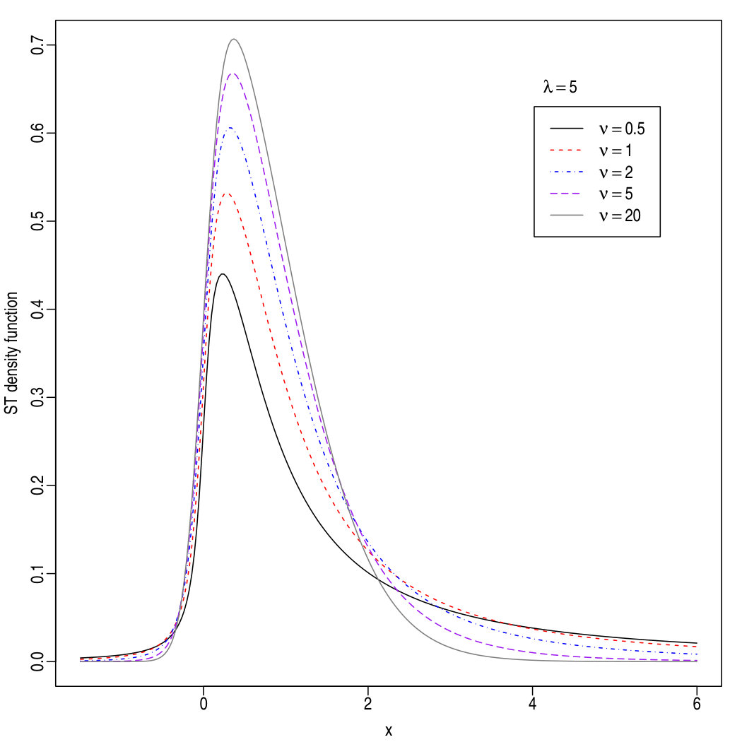 Figure 1
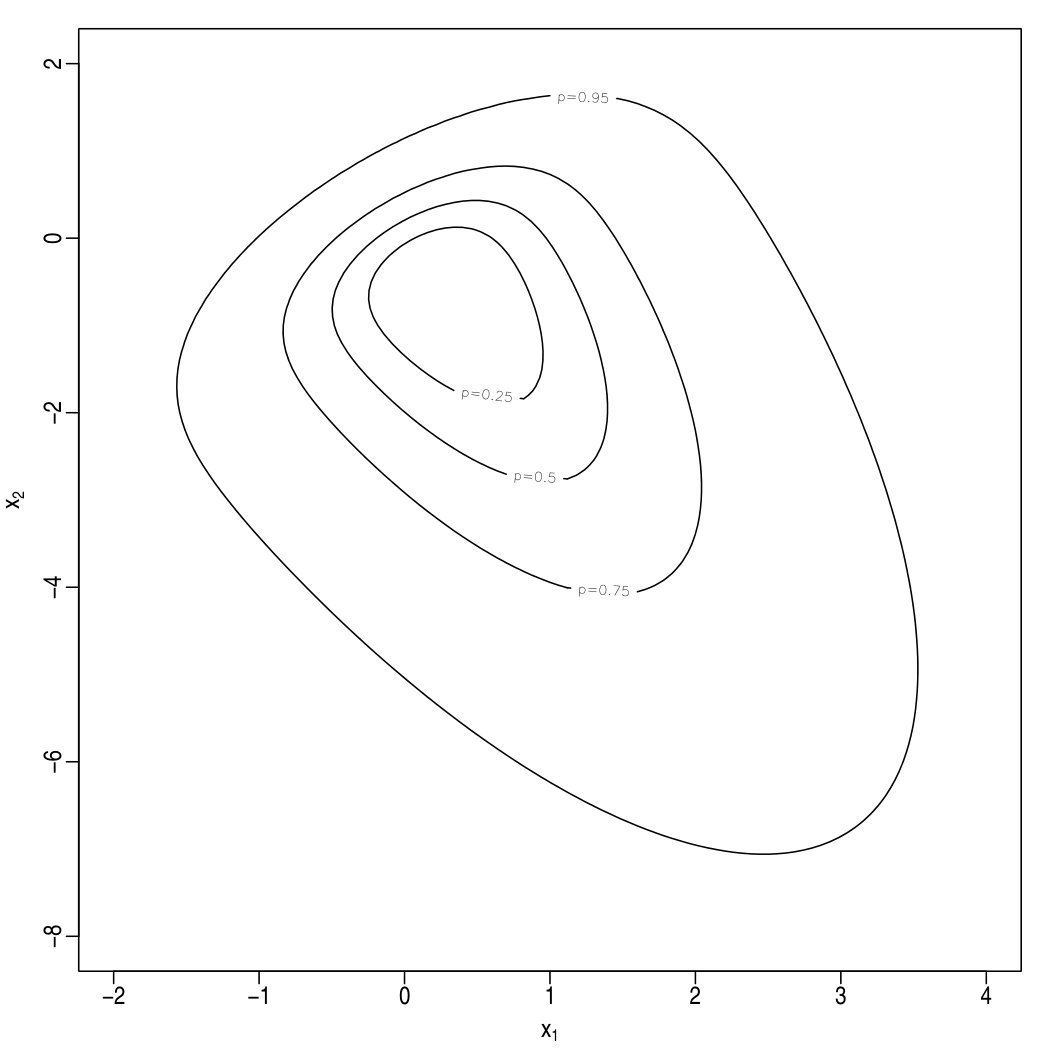 Figure 2
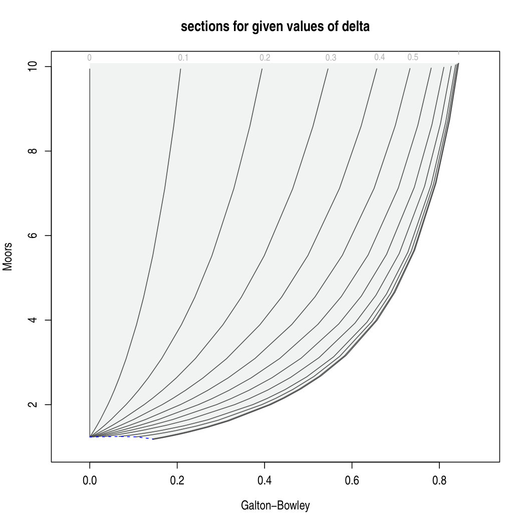 Figure 3
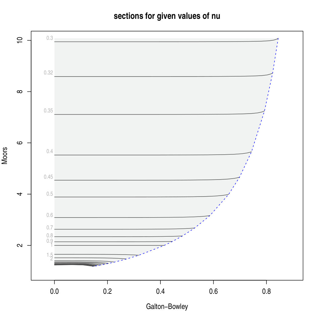 Figure 4
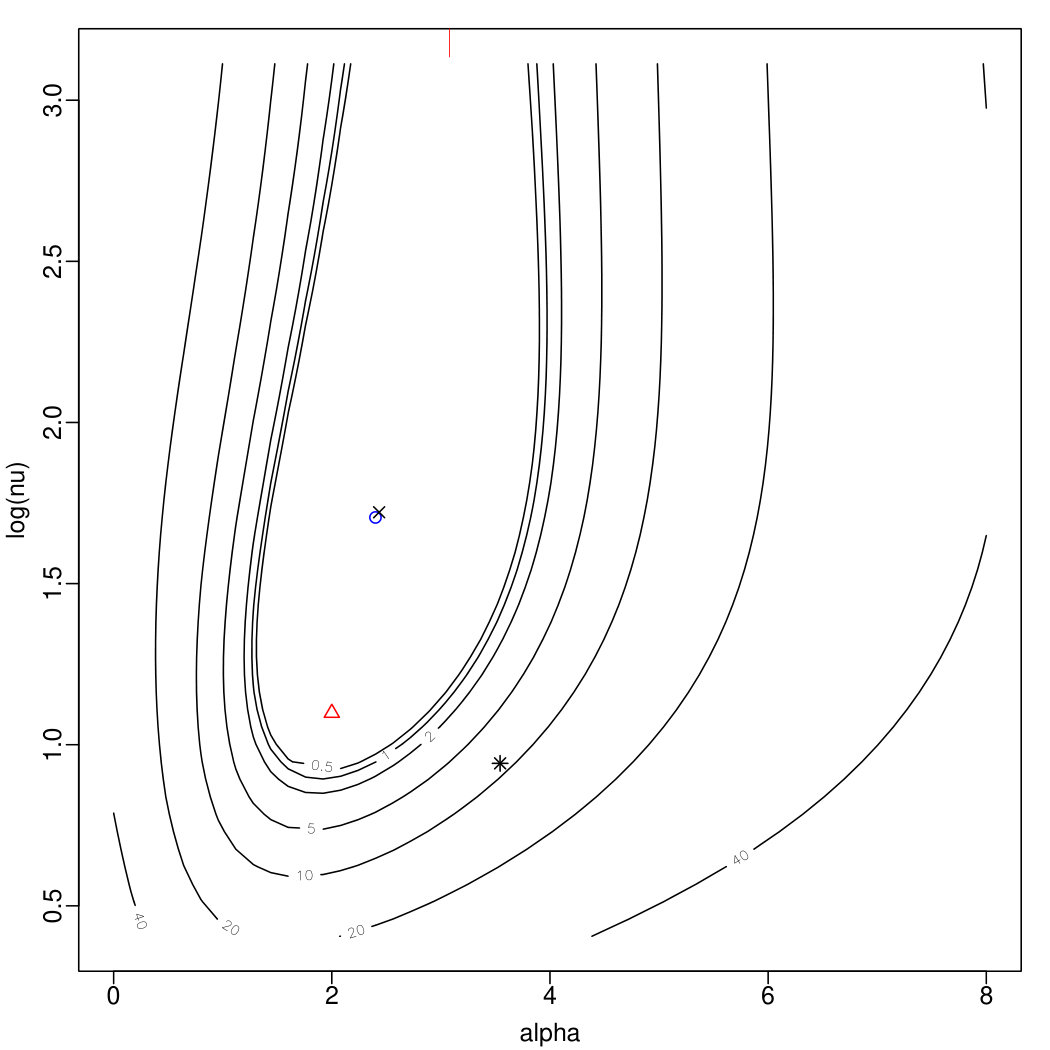 Figure 5
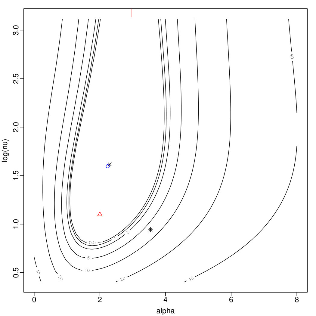 Figure 6
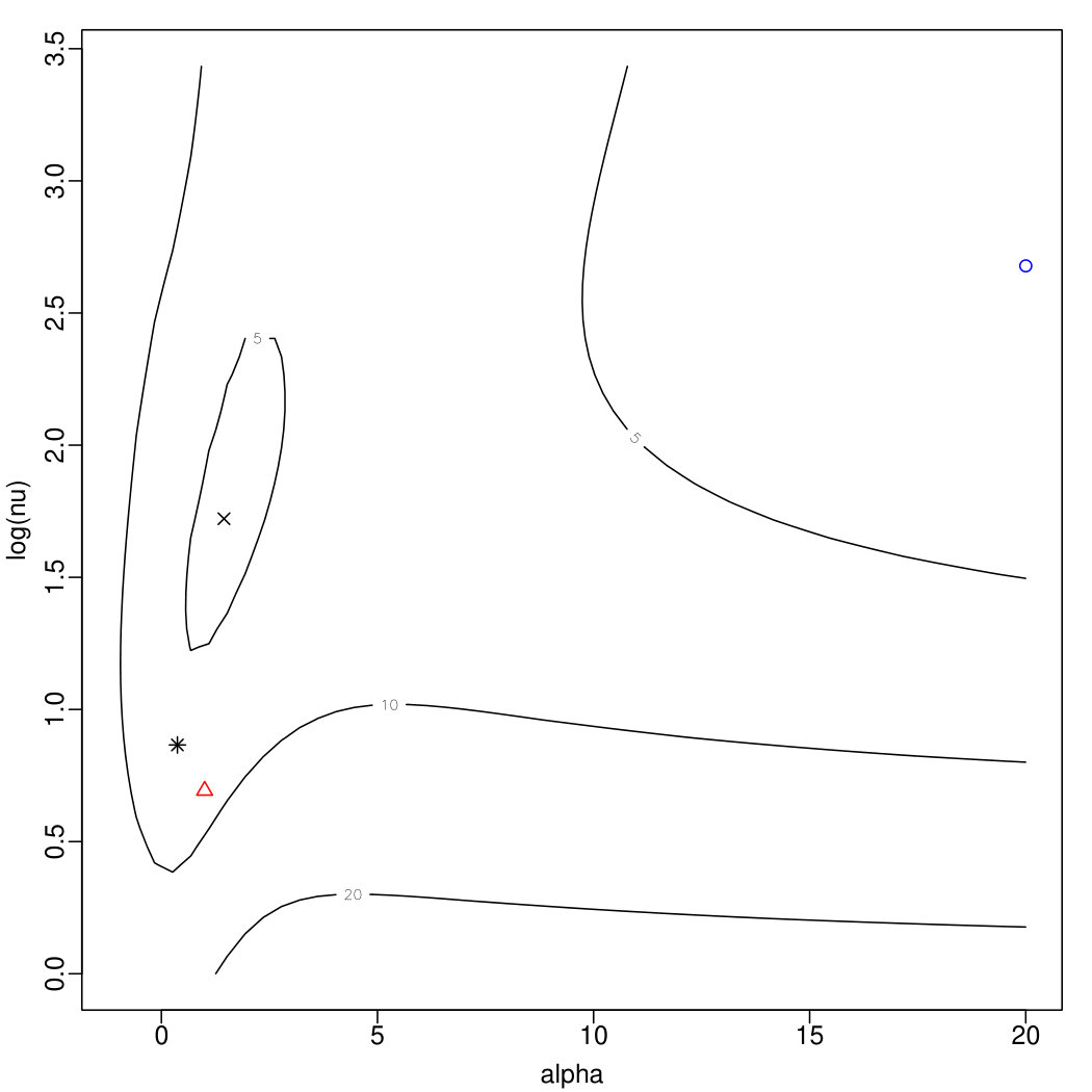 Figure 7
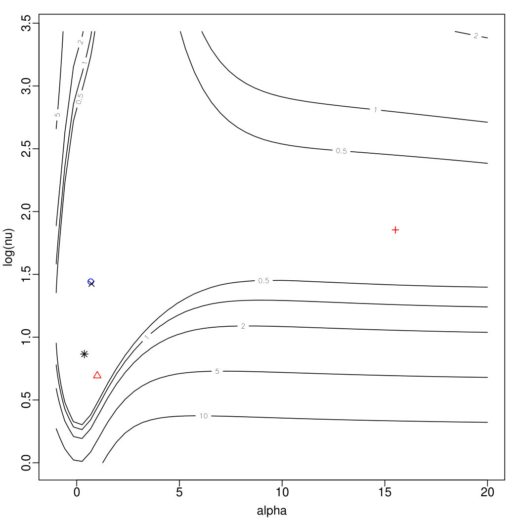 Figure 8
| 0.30 | 9.946 | 2.213831 | 0.315418 | 0.007641 |
| 0.32 | 8.588 | 2.022665 | 0.240821 | 0.012001 |
| 0.35 | 7.110 | 1.790767 | 0.164193 | 0.021492 |
| 0.40 | 5.525 | 1.506418 | 0.090251 | 0.047034 |
| 0.45 | 4.543 | 1.305070 | 0.050702 | 0.087117 |
| 0.50 | 3.888 | 1.156260 | 0.028013 | 0.143526 |
| 0.60 | 3.088 | 0.952435 | 0.005513 | 0.307509 |
| 0.70 | 2.630 | 0.819371 | 0.004209 | 0.536039 |
| 0.80 | 2.339 | 0.724816 | 0.008992 | 0.818739 |
| 0.90 | 2.142 | 0.653206 | 0.011596 | 1.142667 |
| 1.00 | 2.000 | 0.596276 | 0.013136 | 1.495125 |
| 1.50 | 1.652 | 0.417375 | 0.015798 | 3.365100 |
| 2.00 | 1.517 | 0.314104 | 0.016371 | 5.011929 |
| 3.00 | 1.403 | 0.192531 | 0.016274 | 7.304089 |
| 4.00 | 1.354 | 0.123531 | 0.015682 | 8.676470 |
| 5.00 | 1.327 | 0.080123 | 0.014987 | 9.546498 |
| 7.00 | 1.298 | 0.030605 | 0.013674 | 10.561206 |
| 10.00 | 1.277 | 0.003627 | 0.012113 | 11.335506 |
| 15.00 | 1.262 | 0.024611 | 0.010334 | 11.977601 |
| 20.00 | 1.254 | 0.030903 | 0.009149 | 12.343369 |
| 30.00 | 1.247 | 0.031385 | 0.007650 | 12.789281 |
| 40.00 | 1.244 | 0.027677 | 0.006721 | 13.074983 |
| 50.00 | 1.241 | 0.023285 | 0.006079 | 13.284029 |
| 100.00 | 1.237 | 0.005288 | 0.004478 | 13.874691 |
| 1.233 |
| 0 | 0 | 0 | 0 | 39561 | 21049 | 10815 | 575 | |
| 0 | 0 | 0 | 0 | 71998 | 0 | 2 | 0 | |
| 0 | 0 | 0 | 0 | 49086 | 20047 | 2866 | 1 | |
| 0 | 0 | 0 | 0 | 44178 | 21880 | 5942 | 0 | |
| 163 | 2010 | 4629 | 51101 | 13790 | 294 | 13 | 0 | |
| 0 | 30 | 1148 | 50694 | 19679 | 438 | 11 | 0 | |
| 121 | 1487 | 2783 | 46038 | 21451 | 116 | 4 | 0 |
Peer Reviews
No public reviews on file for this paper yet. If you reviewed it on a platform where reviews are public (OpenReview, ICLR, NeurIPS, ICML), you can paste yours below so the community can read it here.
Videos
No videos yet. Explain this paper in a talk, walkthrough, or lecture? Add one.
Taxonomy
TopicsStatistical Distribution Estimation and Applications · Statistical Methods and Bayesian Inference · Advanced Statistical Methods and Models
Some computational aspects of maximum likelihood estimation
of the skew- distribution
Adelchi Azzalini
Dipartimento di Scienze Statistiche
Università di Padova, Italia
Mahdi Salehi
Department of Mathematics and Statistics
University of Neyshabur, Iran
(16th June 2019)
Abstract
Since its introduction, the skew- distribution has received much attention in the literature both for the study of theoretical properties and as a model for data fitting in empirical work. A major motivation for this interest is the high degree of flexibility of the distribution as the parameters span their admissible range, with ample variation of the associated measures of skewness and kurtosis. While this high flexibility allows to adapt a member of the parametric family to a wide range of data patterns, it also implies that parameter estimation is a more delicate operation with respect to less flexible parametric families, given that a small variation of the parameters can have a substantial effect on the selected distribution. In this context, the aim of the present contribution is to deal with some computational aspects of maximum likelihood estimation. A problem of interest is the possible presence of multiple local maxima of the log-likelihood function. Another one, to which most of our attention is dedicated, is the development of a quick and reliable initialization method for the subsequent numerical maximization of the log-likelihood function, both in the univariate and the multivariate context.
1 Background and aims
1.1 Flexible distributions: the skew- case
In the context of distribution theory, a central theme is the study of flexible parametric families of probability distributions, that is, families allowing substantial variation of their behaviour when the parameters span their admissible range. For brevity, we shall refer to this domain with the phrase ‘flexible distributions’. The archetypal construction of this logic is represented by the Pearson system of curves for univariate continuous variables. In this formulation, the density function is regulated by four parameters, allowing wide variation of the measures of skewness and kurtosis, hence providing much more flexibility than in the basic case represented by the normal distribution, where only location and scale can be adjusted.
Since Pearson times, flexible distributions have remained a persistent theme of interest in the literature, with a particularly intense activity in recent years. A prominent feature of newer developments is the increased consideration for multivariate distributions, reflecting the current availability in applied work of larger datasets, both in sample size and in dimensionality. In the multivariate setting, the various formulations often feature four blocks of parameters to regulate location, scale, skewness and kurtosis.
While providing powerful tools for data fitting, flexible distributions also pose some challenges when we enter the concrete estimation stage. We shall be working with maximum likelihood estimation (MLE) or variants of it, but qualitatively similar issues exist for other criteria. Explicit expressions of the estimates are out of the question; some numerical optimization procedure is always involved and this process is not so trivial because of the larger number of parameters involved, as compared with fitting simpler parametric models, such as a Gamma or a Beta distribution. Furthermore, in some circumstances, the very flexibility of these parametric families can lead to difficulties: if the data pattern does not aim steadily towards a certain point of the parameter space, there could be two or more such points which constitute comparably valid candidates in terms of log-likelihood or some other estimation criterion. Clearly, these problems are more challenging with small sample size, later denoted , since the log-likelihood function (possibly tuned by a prior distribution) is relatively more flat, but numerical experience has shown that they can persist even for fairly large , in certain cases.
The focus of interest in this paper will be the skew- (ST) distribution introduced by Branco & Dey, (2001) and studied in detail by Azzalini & Capitanio, (2003); see also Gupta, (2003). The main formal constituents and properties of the ST family will be summarized in the next subsection. Here, we recall instead some of the many publications that have provided evidence of the practical usefulness of the ST family, in its univariate and multivariate version, thanks to its capability to adapt to a variety of data patterns. The numerical exploration by Azzalini & Genton, (2008), using data of various origins and nature, is an early study in this direction, emphasizing the potential of the distribution as a tool for robust inference. The robustness aspects of ST-based inference has also been discussed by (Azzalini & Capitanio,, 2014, § 4.3.5) and more extensively by Azzalini, (2016). On the more applied domain, numerous publications motivated by application problems have further highlighted the ST usefulness, typically with data distributions featuring substantial tailweight and asymmetry. For space reasons, the following list reports only a few of the many publications of this sort, with a preference for early work: Walls, (2005) and Pitt, (2010) use the ST distribution for modelling log-transformed returns of film and music industry products as a function of explanatory variables; Meucci, (2006) and Adcock, (2010) develop methods for optimal portfolio allocation in a financial context, where long tails and asymmetry of returns distribution are standard features; Ghizzoni et al., (2010) use the multivariate ST distributions to model riverflow, jointly at multiple sites; Pyne et al., (2009) present an early model-based clustering formulation using the multivariate ST distributions as the basic component for flow cytometric data analysis.
Given its value in data analysis, but also the above-mentioned possible critical aspects of the log-likelihood function, it seems appropriate to explore the corresponding issues for MLE computation and to develop a methodology which provides good starting points for the numerical maximization of the log-likelihood. After a brief summary of the main facts about the ST distribution in the next subsection, the rest of the paper is dedicated to these issues. Specifically, one section examines qualitatively and numerically various aspects of the ST log-likelihood, while the rest of the paper develops a technique to initialize the numerical search for MLE.
To avoid potential misunderstanding, we underline that the above-indicated program of work does not intend to imply a general inadequacy of the currently available computational resources, which will be recalled in due course. There are, however, critical cases where these resources run into problems, most typically when the data distribution exhibits very long tails. For these challenging situations, an improved methodology is called for.
1.2 The skew- distribution: basic facts
Before entering our actual development, we recall some basic facts about the ST parametric family of continuous distributions. In its simplest description, it is obtained as a perturbation of the classical Student’s distribution. For a more specific description, start from the univariate setting, where the components of the family are identified by four parameters. Of these four parameters, the one denoted in the following regulates the location of the distribution; scale is regulated by the positive parameter ; shape (as departure from symmetry) is regulated by ; tail-weight is regulated by (with ), denoted ‘degrees of freedom’ like for a classical distribution.
It is convenient to introduce the distribution in the ‘standard case’, that is, with location and scale . In this case, the density function is
[TABLE]
where
[TABLE]
is the density function of the classical Student’s on degrees of freedom and denotes its distribution function; note however that in (1) this is evaluated with degrees of freedom. Also, note that the symbol is used for both densities in (1) and (2), which are distinguished by the presence of either one or two parameters.
If is a random variable with density function (1), the location and scale transform has density
[TABLE]
where . In this case, we write , where is squared for similarity with the usual notation for normal distributions.
When , we recover the scale-and-location family generated by the distribution (2). When , we obtain the skew-normal (SN) distribution with parameters , which is described for instance by (Azzalini & Capitanio,, 2014, Chap. 2). When and , (3) converges to the distribution.
Some instances of density (1) are displayed in the left pane of Figure 1. If was replaced by , the densities would be reflected on the opposite side of the vertical axis, since .
Similarly to the classical distribution, moments exist when their order is smaller than . Under this condition, expressions for the mean value, the variance and the coefficients of skewness and excess kurtosis, namely the standardized third and fourth cumulants, are as follows:
[TABLE]
where
[TABLE]
It is visible that, as spans the real line, so does the coefficient of skewness when . For , does not exists; however, at least one of the tails is increasingly heavier as , given the connection with the Student’s . A fairly similar pattern holds for the coefficients of kurtosis , with the threshold at for its existence. If , the range of is ). The feasible space when is displayed in Figure 4.5 of Azzalini & Capitanio, (2014). Negative values are not achievable, but this does not not seem to be a major drawback in most applications.
The multivariate ST density is represented by a perturbation of the classical multivariate density in dimensions, namely
[TABLE]
where is a symmetric positive-definite matrix with unit diagonal elements and . The multivariate version of (1) is then given by
[TABLE]
where is a -dimensional vector regulating asymmetry. An instance of density (6) with is displayed in the right pane of Figure 1 via contour level curves.
Similarly to the univariate setting, we consider the location and scale transformation of a variable with density (6) to where now and is diagonal matrix with positive diagonal elements. For the resulting variable, we use the notation where .
One property required for our later development is that each marginal component of is a univariate ST variable, having a density of type (1) whose parameters are extracted from the corresponding components of , with the exception of for which the marginalization step is slightly more elaborate.
There are many additional properties of the ST distribution which, for space reasons, we do not report here and refer the reader to the quoted literature. A self-contained account is provided by the monograph Azzalini & Capitanio, (2014); see specifically Chapter 4 for the univariate case and Chapter 6 for the multivariate case.
2 On the likelihood function of ST models
2.1 Basic general aspects
The high flexibility of the ST distribution makes it particularly appealing in a wide range of data fitting problems, more than its companion, the SN distribution. Reliable techniques for implementing connected MLE or other estimation methods are therefore crucial.
From the inference viewpoint, another advantage of the ST over the related SN distribution is the lack of a stationary point at (or in the multivariate case), and the implied singularity of the information matrix. This stationary point of the SN is systematic: it occurs for all samples, no matter what is. This peculiar aspect has been emphasized more than necessary in the literature, considering that it pertains to a single although important value of the parameter. Anyway, no such problem exists under the ST assumption. The lack of a stationary point at the origin was first observed empirically and welcomed as ‘a pleasant surprise’ by Azzalini & Capitanio, (2003), but no theoretical explanation was given. Additional numerical evidence in this direction has been provided by Azzalini & Genton, (2008). The theoretical explanation of why the SN and the ST likelihood functions behave differently was finally established by Hallin & Ley, (2012).
Another peculiar aspect of the SN likelihood function is the possibility that the maximum of the likelihood function occurs at , or at in the multivariate case. Note that this happen without divergence of the likelihood function, but only with divergence of the parameter achieving the maximum. In this respect the SN and the ST model are similar: both of them can lead to this pattern.
Differently from the stationarity point at the origin, the phenomenon of divergent estimates is transient: it occurs mostly with small , and the probability of its occurrence decreases very rapidly when increases. However, when it occurs for the available data, we must handle it. There are different views among statisticians on whether such divergent values must be retained as valid estimates or they must be rejected as unacceptable. We embrace the latter view, for the reasons put forward by Azzalini & Arellano-Valle, (2013), and adopt the maximum penalized likelihood estimate (MPLE) proposed there to prevent the problem. While the motivation for MPLE is primarily for small to moderate , we use it throughout for consistency.
There is an additional peculiar feature of the ST log-likelihood function, which however we mention only for completeness, rather than for its real relevance. In cases when is allowed to span the whole positive half-line, poles of the likelihood function must exist near , similarly to the case of a Student’s with unspecified degrees of freedom. This problem has been explored numerically by Azzalini & Capitanio, (2003), and the indication was that these poles must exist at very small values of , such as in one specific instance.
This phenomenon is qualitatively similar to the problem of poles of the likelihood function for a finite mixture of continuous distributions. Even in the simple case of univariate normal components, there always exist poles on the boundary of the parameter space if the standard deviations of the components are unrestricted; see for instance (Day,, 1969, Section 7). The problem is conceptually interesting, in both settings, but in practice it is easily dealt with in various ways. In the ST setting, the simplest solution is to impose a constraint where is some very small value, such as or . Even if fitted to data, a or ST density with would be an object hard to use in practice.
2.2 Numerical aspects and some illustrations
Since, on the computational side, we shall base our work the R package sn, described by Azzalini, (2019), it is appropriate to describe some key aspects of this package.. There exists a comprehensive function for model fitting, called selm, but the actual numerical work in case of an ST model is performed by functions st.mple and mst.mple, in the univariate and the multivariate case, respectively. To numerical efficiency, we shall be using these functions directly, rather than via selm. As their names suggest, st.mple and mst.mple perform MPLE, but they can be used for classical MLE as well, just by omitting the penalty function. The rest of the description refers to st.mple, but mst.mple follows a similar scheme.
In the univariate case, denote by the parameters to be estimated, or possibly when a linear regression model is introduced for the location parameter, in which case is a vector of regression coefficients. Denote by the log-likelihood function at point . If no starting values are supplied, the first operation of st.mple is to fit a linear model to the available explanatory variables; this reduces to the constant covariate value 1 if . For the residuals from this linear fit, sample cumulants of order up to four are computed, hence including the sample variance. An inversion from these values to may or may not be possible, depending on whether the third and fourth sample cumulants fall in the feasible region for the ST family. If the inversion is successful, initial values of the parameters are so obtained; if not, the final two components of are set at , retaining the other components from the linear fit. Starting from this point, MLE or MPLE is searched for using a general numerical optimization procedure. The default procedure for performing this step is the R function nlminb, supplied with the score functions besides the log-likelihood function. We shall refer, comprehensively, to this currently standard procedure as ‘method M0’.
In all our numerical work, method M0 uses st.mple, and the involved function nlminb, with all tuning parameters kept at their default values. The only activated option is the one switching between MPLE and MLE, and even this only for the work of present section. Later on, we shall always use MPLE, with penalty function Qpenalty which implements the method proposed in Azzalini & Arellano-Valle, (2013).
We start our numerical work with some illustrations, essentially in graphical form, of the log-likelihood generated by some simulated datasets. The aim is to provide a direct perception, although inevitably limited, of the possible behaviour of the log-likelihood and the ensuing problems which it poses for MLE search and other inferential procedures. Given this aim, we focus on cases which are unusual, in some way or another, rather than on ‘plain cases’.
The type of graphical display which we adopt is based on the profile log-likelihood function of , denoted . This is obtained, for any given , by maximizing with respect to the remaining parameters. To simplify readability, we transform to the likelihood ratio test statistic, also called ‘deviance function’:
[TABLE]
where is the overall maximum value of the log-likelihood, equivalent to . The concept of deviance applies equally to the penalized log-likelihood.
The plots in Figure 2 displays, in the form of contour level plots, the behaviour of for two artificially generated samples, with expressed on the logarithmic scale for more convenient readability. Specifically, the top plots refer to a sample of size drawn from the ; the left plot, refers to the regular log-likelihood, while the right plot refers to the penalized log-likelihood.
The plots include marks for points of special interest, as follows:
the true parameter point;
the point having maximal (penalized) log-likelihood on a grid of points spanning the plotted area;
the MLE or MPLE point selected by method M0;
the preliminary estimate to be introduced in Section 3.2, later denoted M1;
the MLE or MPLE point selected by method M2 presented later in the text.
It will be noticed that the top-left plot does not show a mark. This is because the MLE point delivered by M0 has (actually some huge values representing numerical ‘approximations of infinity’), where ; consequently the maximum of over the plotted area takes place at its margin. Note that the log-likelihood function has a local maximum at about , where ; this local maximum is quite close to the true parameter point, especially so in the light of the limited sample size. There are two messages from this example: one is that the log-likelihood may have more than one maximum; the other is that a local maximum can provide a better choice than the global maximum, at least in this case.
Given that , consider MPLE estimation in the top-right plot. The maximum of , marked by , is now close to the point , but method M0 fails to find it, and it picks up the point . This must be due to a poor choice of the initial point for numerical search, given that method M2, which differs only for this initial point, lands on the correct point.
Peculiar behaviours, either of the log-likelihood or of the estimation procedures or both of them, are certainly more frequent when is small or moderate, but problems can persist even for fairly large , as illustrated by the bottom two plots of Figure 2 which refer to a sample of size from . In this case, M0 yields and , denoted by the vertical ticks below the top side of the plotted area; the associated value is for the left plot, for the right plot. Both these values are lower than the corresponding maximal values, and . Again, better initial search points used by method M2 leads to the correct global maxima, at about and , respectively.
3 On the choice of initial parameters for MLE search
The aim of this section, which represents the main body of the paper, is to develop a methodology for improving the selection of initial parameter values from where to start the MPLE search via some numerical optimization technique, which should hopefully achieve a higher maximum.
3.1 Preliminary remarks and the basic scheme
We have seen in Section 2 the ST log-likelihood function can be problematic; it is then advisable to select carefully the starting point for the MLE search. While contrasting the risk of landing on a local maximum, a connected aspect of interest is to reduce the overall computing time. Here are some preliminary considerations about the stated target.
Since these initial estimates will be refined by a subsequent step of log-likelihood maximization, there is no point in aiming at a very sophisticate method. In addition, we want to keep the involved computing header as light as possible. Therefore, we want a method which is simple and quick to compute; at the same time, it should be reasonably reliable, hopefully avoiding nonsensical outcomes.
Another consideration is that we cannot work with the methods of moments, or some variant of it, as this would impose a condition , bearing in mind the constraints recalled in Section 1.2. Since some of the most interesting applications of ST-based models deal with very heavy tails, hence with low degrees of freedom, the condition would be unacceptable in many important applications. The implication is that we have to work with quantiles and derived quantities.
To ease exposition, we begin by presenting the logic in the basic case of independent observations from a common univariate distribution . The first step is to select suitable quantile-based measures of location, scale, asymmetry and tail-weight. The following list presents a set of reasonably choices; these measures can be equally referred to a probability distribution or to a sample, depending on the interpretation of the terms quantile, quartile and alike.
Location
The median is the obvious choice here; denote it by , since it coincides with the second quartile.
Scale
A commonly used measure of scale is the semi-interquartile difference, also called quartile deviation, that is
[TABLE]
where denotes the th quartile; see for instance (Kotz et al.,, 2006, vol. 10, p. 6743).
Asymmetry
A classical non-parametric measure of asymmetry is the so-called Bowley’s measure
[TABLE]
see (Kotz et al.,, 2006, vol. 12, p. 7771–3). Since the same quantity, up to an inessential difference, had previously been used by Galton, some authors attribute to him its introduction. We shall refer to as the Galton-Bowley measure.
Kurtosis
A relatively more recent proposal is the Moors measure of kurtosis, presented in Moors, (1988),
[TABLE]
where denotes the th octile, for . Clearly, for .
A key property is that is independent of the location of the distribution, and and are independent of location and scale.
For any distribution , the values of are functions of the parameters . Given a set of observations drawn from under mutual independence condition, we compute sample values of of from the sample quantiles and then inversion of the functions connecting and will yield estimates of the ST parameters. In essence, the logic is similar to the one underlying the method of moments, but with moments replaced by quantiles.
In the following subsection, we discuss how to numerically carry out the inversion from to . Next, we extend the procedure to settings which include explanatory variables and multivariate observations.
3.2 Inversion of quantile-based measures to ST parameters
For the inversion of the parameter set to , the first stage considers only the components which are to be mapped to , exploiting the invariance of and with respect to location and scale. Hence, at this stage, we can work assuming that and .
Start by computing, for any given pair , the set of octiles of , and from here the corresponding values. Operationally, we have computed the ST quantiles using routine qst of package sn. Only non-negative values of need to be considered, because a reversal of the sign simply reverses the sign of , while is unaffected, thanks to the mirroring property of the ST quantiles when is changed to .
Initially, our numerical exploration of the inversion process examined the contour level plots of and as functions of and , as this appeared to be the more natural approach. Unfortunately, these plots turned out not to be useful, because of the lack of a sufficiently regular pattern of the contour curves. Therefore these plots are not even displayed here.
A more useful display is the one adopted in Figure 3, where the coordinate axes are now and . The shaded area, which is the same in both panels, represents the set of feasible points for the ST family. In the first plot, each of the black lines indicates the locus of points with constant values of , defined by (4), when spans the positive half-line; the selected values are printed at the top of the shaded area, when feasible without clutter of the labels. The use of instead of simply yields a better spread of the contour lines with different parameter values, but it is conceptually irrelevant. The second plot of Figure 3 displays the same admissible region with superimposed a different type of loci, namely those corresponding to specified values of , when spans the interval; the selected values are printed on the left side of the shaded area.
Details of the numerical calculations are as follows. The Galton-Bowley and the Moors measures have been evaluated over a grid of points identified by the selected values
[TABLE]
The and values so obtained form the basis of Figure 3 and subsequent calculations. Note that, while the vectors and identify a regular grid of points on the space, they corresponds to a curved grid on the shaded regions of Figure 3.
Boundary parameter values require a special handling. Specifically, and correspondingly identify the Student’s distribution truncated below 0, that is, the square root transform of the Snedecor’s distribution; hence, in this case the quantiles are computed as square roots of the quantiles. The associated points lie on the right-side boundary of the shaded area. Another special value is which corresponds to the SN distribution. In this case, function qsn of package sn has been used; the corresponding points lie on the concave curve in the bottom-left corner of the shaded area.
Conceptually, Figure 3 represents the key for the inversion from to and equivalently to since . However, in practical terms, we must devise a mechanism for inversely interpolating the values computed at the grid points. Evaluation of this interpolation scheme at the sample values will yield the desired estimates.
To this end, the second plot indicates the most favourable front for tackling the problem, since its almost horizontal lines show that the Moors measure is very nearly a function of only. Denote by the value of when . The 25 available values of at are reported in the second column of Table 1; the remaining columns will be explained shortly. From these 25 values, an interpolating spline of as a function of has been introduced. Use of the transformed variable substantially reduces the otherwise extreme curvature of the function. Evaluation of this spline function at the sample value and conversion into its reciprocal yields an initial estimate .
Consider now estimation of or equivalently of , a task which essentially amounts to approximate the curves in the first plot in Figure 3. After some numerical exploration, it turned out that a closely interpolating function can be established in the following form:
[TABLE]
where the fitted values of the coefficients for the selected values are reported in the last three columns of Table 1, with the exception of . Use of (8) combined with the coefficients of Table 1 allows to find an approximate value of for the selected values of . If an intermediate value of must be considered, such that where are two adjacent values of , a linear interpolation of the corresponding coefficients is performed. More explicitly, a value of is obtained by linear interpolation of and , for ; then (8) is applied using these interpolated coefficients. If is outside the range of finite values in the first column of Table 1, the values associated to the closest such value of are used.
Operationally, we use the just-described scheme with set at the value obtained earlier, leading to an estimate of .
Numerical testing of this procedure has been performed as follows. For a number of pairs of values , the corresponding octiles and the measures have been computed and the proposed procedure has been applied to these measures. The returned parameter values were satisfactorily close to the original pair, with some inevitable discrepancies due to the approximations involved, but of limited entity. If necessary, a refinement can be obtained by numerical search targeted to minimize a suitable distance between a given pair and the analogous values derived from the associated pair. However, this refinement was not felt necessary in the numerical work described later, thanks to the good working of the above-described interpolation scheme.
We are now left with estimation of and . Bearing in mind the representation introduced just before (3), is naturally estimated by
[TABLE]
where the terms in the numerator are sample quartiles and those in the denominator are quartiles of .
Consideration of again says that an estimate of can be obtained as an adjustment of the sample median via
[TABLE]
where is the median of .
The estimates so produced are marked by an asterisk in the examples of Figure 2, showing to perform well in those cases, while requiring a negligible computing time compared to MLE.
3.3 Extension to the regression case
We want to extend the methodology of Section 3.2 to the regression setting where the location parameter varies across observations as a linear function of a set of , say, explanatory variables, which are assumed to include the constant term, as it is commonly the case. If is the vector of covariates pertaining to the th subject, observation is now assumed to be drawn from where
[TABLE]
for some -dimensional vector of unknown parameters; hence now the parameter vector is . The assumption of independently drawn observations is retained.
The direct extension of the median as an estimate of location, which was used in Section 3.2, is an estimate of obtained by median regression, which corresponds to adoption of the least absolute deviations fitting criterion instead of the more familiar least squares. This can also be viewed as a special case of quantile regression, when the quantile level is set at . A classical treatment of quantile regression is Koenker, (2005) and corresponding numerical work can be carried out using the R package quantreg, see Koenker, (2018), among others tools.
Use of median regression delivers an estimate of and a vector of residual values, for . Ignoring estimation errors, these residuals are values sampled from , where is a suitable value, examined shortly, which makes the distribution to have 0 median, since this is the target of the median regression criterion. We can then use the same procedure of Section 3.2, with the ’s replaced the ’s, to estimate , given that the value of is irrelevant at this stage.
The final step is a correction to the vector to adjust for the fact that should have median , that is, the median of , not median 0. This amounts to increase all residuals by a constant value , and this step is accomplished by setting a vector with all components equal to except that the intercept term, say, is estimated by
[TABLE]
similarly to (10).
3.4 Extension to the multivariate case
Consider now the case of independent observations from a multivariate variable with density (6), hence . This case can be combined with the regression setting of Section 3.3, so that the -dimensional location parameter varies for each observation according to
[TABLE]
where now is a matrix of parameters. Since we have assumed that the explanatory variables include a constant term, the regression case subsumes the one of identical distribution, when . Hence we deal with the regression case directly, where the th observation is sampled from and is given by (12), for .
Arrange the observed values in a matrix . Application of the procedure presented in Sections 3.2 and 3.3 separately to each column of delivers estimates of univariate models. Specifically, from the th column of , we obtain estimates and corresponding ‘normalized’ residuals :
[TABLE]
where it must be recalled that the ‘normalization’ operation uses location and scale parameters, but these do not coincide with the mean and the standard deviation of the underlying random variable.
Since the meaning of expression (12) is to define a set of univariate regression modes with a common design matrix, the vectors can simply be arranged in a matrix which represents an estimate of .
The set of univariate estimates in (13) provide estimates for , while only one such a value enters the specification of the multivariate ST distribution. We have adopted the median of as the single required estimate, denoted .
The scale quantities estimate the square roots of the diagonal elements of , but off-diagonal elements require a separate estimation step. What is really required to estimate is the scale-free matrix . This is the problem examined next.
If is the diagonal matrix formed by the squares roots of , all variables have distribution , for . Denote by the generic member of this set of variables. We are concerned with the distribution of the products , but for notational simplicity we focus on the specific product , since all other products are of similar nature.
We must then examine the distribution of when is a bivariate ST variable. This looks at first to be a daunting task, but a major simplification is provided by consideration of the perturbation invariance property of symmetry-modulated distributions, of which the ST is an instance. For a precise exposition of this property, see for instance Proposition 1.4 of Azzalini & Capitanio, (2014), but in essence it states that, since is an even function of , its distribution does not depend on , and it coincides with the distribution of the case , that is, the case of a usual bivariate Student’s distribution, with dependence parameter .
Denote by the distribution function of the product of variables having bivariate Student’s density (5) in dimension with degrees of freedom and dependence parameter where . An expression of is available in Theorem 1 of Wallgren, (1980). Although this expression involves numerical integration, this is not problematic since univariate integration can be performed efficiently and reliably with the R function integrate.
To estimate , we search for the value of such that the median of the distribution of equates its sample value. In practice, we compute the sample values where , using the residuals in (13), and denote their median by . Then we must numerically solve the non-linear equation
[TABLE]
with respect to . Solution of the equation is facilitated by the monotonicity of with respect to , ensured by Theorem 2 of Wallgren, (1980). The solution of (14) is the estimate .
Proceeding similarly for other pairs of variables , all entries of matrix can be estimated; the diagonal elements are all 1. However, it could happen that the matrix so produced is not a positive-definite correlation matrix, because of estimation errors. Furthermore an even more stringent condition has to be satisfied, namely that
[TABLE]
This condition on applies to all skew-elliptical distributions, of which the ST is an instance; see (Branco & Dey,, 2001, p. 101) or (Azzalini & Capitanio,, 2014, p. 171).
Denote by the estimate of with in the top-left block obtained by solutions of equations of type (14) and computed by applying in (4) to . If is positive definite, then we move on to the next step; otherwise an adjustment is required.
There exist various techniques to adjust a nearly positive-definite matrix to achieve positive-definiteness. Some numerical experimentation has been carried out using procedure nearPD of R package Matrix; see Bates & Maechler, (2019). Unfortunately, this did not work well when we used the resulting matrix for the next step, namely computation of the vector
[TABLE]
which enters the density function (6); see for instance equation (4) of Azzalini & Capitanio, (2003), which is stated for the SN distribution, but it holds also for the ST. The unsatisfactory outcome from nearPD for our problem is presumably due to modifications in the relative size of the components of , leading to grossly inadequate vectors, typically having a gigantic norm.
A simpler type of adjustment has therefore been adopted, as follows. If condition (15) does not hold for , the off-diagonal elements of the matrix are shrunk by a factor 0.95, possibly repeatedly, until (15) is satisfied. This procedure was quick to compute and it did not cause peculiar outcomes from (16).
Hence, either directly from the initial estimates of and or after the adjustment step just described, we obtain valid components satisfying condition (15) and a corresponding vector from (16). The final step is to introduce scale factors via
[TABLE]
where . This completes estimation of .
3.5 Simulation work to compare initialization procedures
A number of simulation runs has been performed to examine the performance of the proposed methodology. The computing environment is R version 3.6.0. The reference point for these evaluations is the methodology currently in use, as provided by the publicly available version of R package sn at the time of writing, namely version 1.5-4; see Azzalini, (2019). This will be denoted ‘the current method’ in the following. Since the role of the proposed method is to initialize the numerical MLE search, not the initialization procedure per se, we compare the new and the current method with respect to final MLE outcome. However, since the numerical optimization method used after initialization is the same, any variations in the results originate from the different initialization procedures.
We stress again that in a vast number of cases the working of the current method is satisfactory and we are aiming at improvements when dealing with ‘awkward samples’. These commonly arise with ST distributions having low degrees of freedom, about or even less, but exceptions exist, such as the second sample in Figure 2.
The primary aspect of interest is improvement in the quality of data fitting. This is typically expressed as an increase of the maximal achieved log-likelihood, in its penalized form. Another desirable effect is improvement in computing time.
The basic set-up for such numerical experiments is represented by simple random samples, obtained as independent and identically distributed values drawn from a named . In all cases we set and . For the other ingredients, we have selected the following values:
[TABLE]
and, for each combination of of these values, samples have been drawn.
The smallest examined sample size, , must be regarded as a sort of ‘sensible lower bound’ for realistic fitting of flexible distributions such as the ST. In this respect, recall the cautionary note of (Azzalini & Capitanio,, 2014, p. 63) about the fitting of a SN distribution with small sample sizes. Since the ST involves an additional parameter, notably one having strong effect on tail behaviour, that annotation holds a fortiori here.
For each of the samples so generated, estimation of the parameters has been carried out using the following methods.
M0: this is the current method, which maximizes the penalized log-likelihood using function st.mple as described in Section 2.2.
M1: preliminary estimates are computed as described in Section 3.2;
M2: maximization of the penalized log-likelihood, still using function st.mple, but starting from the estimates of M1;
M3: similar to M2, but using a simplified form of M1, where only the location and scale parameters are estimated, setting and .
An exhaustive analysis of the simulation outcome would be far too lengthy and space consuming. As already mentioned, our primary interest is on the differences of maximized log-likelihood. Specifically, if denote by the maximized value of the penalized log-likelihood using method M, we focus on the quantities , and , where . Table 2 reports the observed frequencies of values, grouped in intervals
[TABLE]
crosstabulated either with or with .
We are not concerned with samples having values in the interval , since these differences are not relevant from an inferential viewpoint; just note that they constitute the majority of cases. As for , the fraction of cases falling outside is small, but it is not negligible, and this justifies our efforts to improve over M0. As expected, larger values occur more easily when or are small, but sometimes also otherwise. In all but a handful of cases, these larger differences are on the positive sides, confirming the effectiveness of the proposed method for initialization. The general indication is that both methods M2 and M3, and implicitly so M1, improve upon the current method M0.
Visual inspections of individual cases where M1 performs poorly indicates that the problem originates in the sample octiles, on which all the rest depends. Especially with very low and/or , the sample octiles can occasionally happen to behave quite differently from expectations, spoiling everything. Unfortunately, there is no way to get around this problem, which however is sporadic.
Another indication from Table 2 is that M3 is essentially equivalent to M2, in terms of maximized log-likelihood, and in some cases it is even superior, in spite of its simplicity.
Another aspect is considered is Table 3 which reports computing times and their differences as frequencies of time intervals. A value represents the computing time for estimation from a given sample using method M, obtained by the first value reported by the R function system.time. For M2 and M3, includes the time spent for initialization with M1, although this is a very minor fraction of the overall time. Clearly the samples considered are of quite different nature, especially so for sample size. However, our purpose is solely comparative and, since exactly the same samples are processed by the various methods, the comparison of average computing times is valid. Table 3 shows a clear advantage of M2 over M0 in terms of computing time and also some advantage, but less prominent, over M3.
Additional simulations have been run having the location parameter expressed via a linear regression. Given a vector formed by equally spaced points on the interval , design matrices have been built using transformations , inclusive of the constant function , as follows:
[TABLE]
Computation of over the values of yields the columns of the design matrix; the regression parameters have been set at for all s. For each of the A, B, C design matrices, and for each parameter combinations in (17), have been generated, similarly to the case of simple random samples.
In Table 4, we summarize results only for case C, as the other cases are quite similar. The distribution of in the top two sub-tables still indicate a superiority of M2 over M0, although less pronounced than for simple samples. The lower portion of the table indicates a slight superiority of M3 over M2, reinforcing the similar indication from Table 2.
In the two subtables of Table 4 about , note that there are 160 samples where M0 goes completely wrong. All these sample were generated with , a fact which is not surprising considering the initial parameter selection of st.mple, in its standard working described at the beginning of Section 2.2. Since that initial selection is based on a least-squares fit of the regression parameters, this step clashes with the non-existence of moments when the underlying ST distribution has degrees of freedom. Not only the regression parameters are poorly fitted, but the ensuing residuals are spoiled, affecting also the initial fit of the other parameters.
A set of simulations has also been run in the bivariate case, hence sampling from density (6) with . The scale matrix and the shape vector have been set to
[TABLE]
where spans the values given in (17). Also and have been set like in (17), with the exception that has been not included, considering that data points would constitute a too small sample in the present context. On the whole, bivariate samples have then been generated. They have been processed by function mst.mple of package sn and the initialization method of Section 3.4, with obvious modifications of the meaning of notation M0 to M3.
The summary output of the simulations is presented in Table 5. There is a clear winner this time, since M3 is constantly superior to the others. Between M0 and M2, the latter is still preferable for , but not otherwise.
The almost constant superiority of M3 over M2 is quite surprising, given the qualitatively different indication emerging in the univariate case. This rather surprising effect must be connected to transformation (16), as it has also been indicated by direct examination of a number of individual cases: a moderate estimation error even of a single component, and consequently of , transforms into a poor estimate of . It so happens that the conservative choice of M3 avoids problems and can be, in its simplicity, more effective.
3.6 Conclusions
The overall indication of the simulation work is that the proposed preliminary estimates work quite effectively, providing an improved initialization of the numerical MPLE search. The primary aspect is that higher log-likelihood values are usually achieved, compared to the currently standard method, M0, sometimes by a remarkable margin. Another positive aspect is the saving in the overall computing time.
Of the two variant forms of the new initialization, leading to methods M2 and M3, the latter has emerged as clearly superior in the multivariate case, but no such clear-cut conclusion can be drawn in the univariate setting, with indications somewhat more favourable for M2. In this case, it is advisable to consider both variant of the preliminary estimates and carry out two numerical searches. Having to choose between them, the quick route is to take the one with higher log-likelihood. However, direct inspection of both outcomes must be recommended, including exploration of the profile log-likelihood surface.
Surely, it would have been ideal to identify a universally superior method, to be adopted for all situations, but this type of simplification still eludes us.
The reference list from the paper itself. Each links out to its DOI / PubMed record.
- 1Adcock, (2010) Adcock, C. J. (2010). Asset pricing and portfolio selection based on the multivariate extended skew-Student- t 𝑡 t distribution. Ann. Oper. Res. , 176(1), 221–234.
- 2Azzalini, (2016) Azzalini, A. (2016). Flexible distributions as an approach to robustness: the skew- t 𝑡 t case. In C. Agostinelli, A. Basu, P. Filzmoser, & D. Mukherjee (Eds.), Recent Advances in Robust Statistics: Theory and Applications chapter 1, (pp. 1–16). Springer India.
- 3Azzalini, (2019) Azzalini, A. (2019). The R package sn : The Skew-Normal and Related Distributions such as the Skew- t 𝑡 t (version 1.5-4). Università di Padova, Italia.
- 4Azzalini & Arellano-Valle, (2013) Azzalini, A. & Arellano-Valle, R. B. (2013). Maximum penalized likelihood estimation for skew-normal and skew- t 𝑡 t distributions. J. Statist. Plann. Inference , 143(2), 419–433. Available online 30 June 2012.
- 5Azzalini & Capitanio, (2003) Azzalini, A. & Capitanio, A. (2003). Distributions generated by perturbation of symmetry with emphasis on a multivariate skew t 𝑡 t distribution. J. R. Statist. Soc., ser. B , 65(2), 367–389. Full version of the paper at ar Xiv.org:0911.2342 .
- 6Azzalini & Capitanio, (2014) Azzalini, A. & Capitanio, A. (2014). The Skew-Normal and Related Families . IMS monographs. Cambridge, UK: Cambridge University Press.
- 7Azzalini & Genton, (2008) Azzalini, A. & Genton, M. G. (2008). Robust likelihood methods based on the skew- t 𝑡 t and related distributions. Int. Statist. Rev. , 76, 106–129.
- 8Bates & Maechler, (2019) Bates, D. & Maechler, M. (2019). Matrix: Sparse and Dense Matrix Classes and Methods . R package version 1.2-17.