TL;DR
This paper introduces a supervised LSTM-based similarity measurement combined with spectral clustering to enhance speaker diarization, significantly reducing error rates compared to existing methods.
Contribution
It presents a novel supervised Bi-LSTM approach for similarity measurement in speaker diarization, integrated with spectral clustering for improved accuracy.
Findings
Achieved a diarization error rate of 6.63% on NIST SRE 2000 CALLHOME.
Outperformed state-of-the-art methods in speaker diarization tasks.
Demonstrated the effectiveness of supervised LSTM in similarity scoring.
Abstract
More and more neural network approaches have achieved considerable improvement upon submodules of speaker diarization system, including speaker change detection and segment-wise speaker embedding extraction. Still, in the clustering stage, traditional algorithms like probabilistic linear discriminant analysis (PLDA) are widely used for scoring the similarity between two speech segments. In this paper, we propose a supervised method to measure the similarity matrix between all segments of an audio recording with sequential bidirectional long short-term memory networks (Bi-LSTM). Spectral clustering is applied on top of the similarity matrix to further improve the performance. Experimental results show that our system significantly outperforms the state-of-the-art methods and achieves a diarization error rate of 6.63% on the NIST SRE 2000 CALLHOME database.
Click any figure to enlarge with its caption.
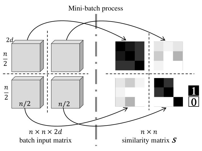 Figure 1
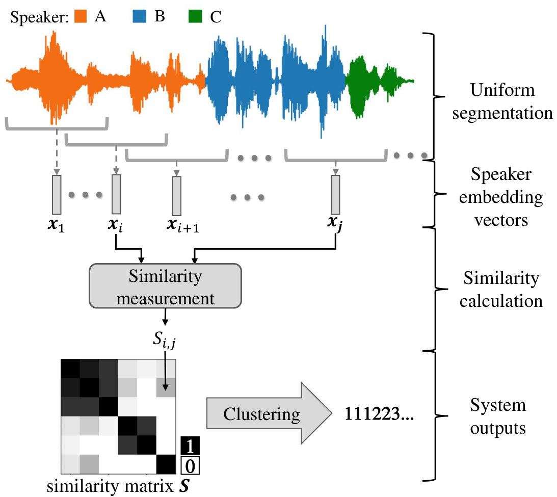 Figure 2
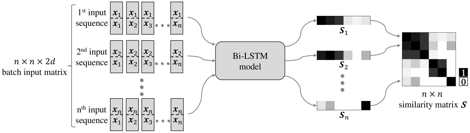 Figure 3
| System architecture | DER(%) | |
| Baseline | i-vector + PLDA + AHC | 10.42 |
| x-vector + PLDA + AHC | 8.64 | |
| SC backend | i-vector + PLDA + SC | 10.13 |
| x-vector + PLDA + SC | 8.05 | |
| LSTM scoring | (1) i-vector + LSTM + SC | 8.53 |
| (2) x-vector + LSTM + SC | 7.73 | |
| (1+2) system fusion | 6.63 | |
| Recent works | Wang et al. [6] | 12.0 |
| Sell at al. [23] | 11.5 | |
| Romero et al. [10] | 9.9 | |
| Zhang et al. [16] (5-fold) | 7.6 |
| sorted utterances | t-value | |||
|---|---|---|---|---|
| 6.6 | 5.5 | -1.22 | accepted | |
| 5.7 | 5.3 | -0.35 | accepted | |
| 6.1 | 3.9 | -2.16 | rejected | |
| 9.2 | 7.5 | -2.11 | rejected | |
| 13.9 | 11.6 | -2.38 | rejected |
Peer Reviews
No public reviews on file for this paper yet. If you reviewed it on a platform where reviews are public (OpenReview, ICLR, NeurIPS, ICML), you can paste yours below so the community can read it here.
Code & Models
Videos
No videos yet. Explain this paper in a talk, walkthrough, or lecture? Add one.
Taxonomy
MethodsSpectral Clustering
LSTM based Similarity Measurement with Spectral Clustering
for Speaker Diarization
Abstract
More and more neural network approaches have achieved considerable improvement upon submodules of speaker diarization system, including speaker change detection and segment-wise speaker embedding extraction. Still, in the clustering stage, traditional algorithms like probabilistic linear discriminant analysis (PLDA) are widely used for scoring the similarity between two speech segments. In this paper, we propose a supervised method to measure the similarity matrix between all segments of an audio recording with sequential bidirectional long short-term memory networks (Bi-LSTM). Spectral clustering is applied on top of the similarity matrix to further improve the performance. Experimental results show that our system significantly outperforms the state-of-the-art methods and achieves a diarization error rate of 6.63% on the NIST SRE 2000 CALLHOME database.
Index Terms: Speaker diarization, segments similarity measurement, Bi-LSTM, PLDA, spectral clustering
1 Introduction
Speaker diarization is the task of determining “who speaks when” in an audio file that usually contains an unknown number of speakers with variable speech duration [1, 2].
Diarization systems are usually made of multiple submodules. First, a voice activity detector (VAD) [3] removes non-speech regions from the audio input. Then, speech regions are split into multiple speaker-homogeneous segments either with a speaker change detector (SCD) [4, 5] or based on uniform segmentation [6]. These segments are mapped into a fixed-dimensional feature space by speaker embedding systems such as i-vector [7, 8], x-vector [9, 10], or penultimate layer output from various end-to-end speaker verification methods [11, 12]. Next, pairwise similarity measurement techniques like cosine distance and PLDA [8, 13] compute the similarity matrix between segments. Finally, agglomerative hierarchical clustering (AHC) [14], spectral clustering [6] or affinity propagation [15] are applied on top of the similarity matrix to obtain the final diarization results.
While the performance of speech recognition and speaker verification systems has improved dramatically thanks to deep learning approaches, most speaker diarization systems have not yet taken full advantage of these techniques. One reason is that speaker diarization labels are ambiguous: both “111223” and “222113” sequences can be equally correct sequences of labels for the same audio input file. Because it is usually addressed as an unsupervised task, the clustering step makes it difficult to design fully supervised diarization system. Zhang [16] did propose the UIS-RNN model for clustering and improved the performance, but UIS-RNN is essentially a mixture of LSTMs and parametric models, and relies heavily on the effectiveness of the speaker embedding front-end.
In this work, we propose to use Bi-LSTM in place of PLDA to model the similarity between any arbitrary two segments. Since PLDA scores similarity between two segments in a pairwise and independent manner, it completely ignores the sequential order of speech segments. However, conversations between several speakers are usually highly structured, and turn-taking behaviors are not randomly distributed over time. In [17], structured prediction is applied for online speaker diarization, but only the structural information from the forward direction is considered. We propose to use both forward and backward segments to overcome such limitations and enhance the performance of similarity measurement. Besides, we use spectral clustering on top of the similarity matrix to obtain the final results.
The rest of this paper is organized as follows. The next section presents the general diarization system overview including speaker embedding extraction, similarity measurement and clustering algorithms. Section 3 describes the details of our Bi-LSTM based similarity measurement module. Experimental results and discussions are presented in Section 4 and conclusions are drawn in Section 5.
2 System overview
In this paper, an oracle VAD is employed to remove non-speech regions in audios. An overview of our system framework is shown in Figure 1. First, we employ uniform segmentation and extract -dimensional speaker embedding vectors from assumedly speaker-homogeneous segments with pre-trained speaker embedding models. Second, a similarity measurement algorithm computes the score between every embedding vector pair and form a square similarity matrix . Finally, we perform clustering among all segments based on . Related algorithms are briefly introduced in this section.
2.1 Speaker embedding vectors
2.1.1 i-vector
i-vector is one of the most widely used speaker embedding vector. Essential components in the i-vector system include the universal background model (UBM) and the total variability space . For a pre-trained system, mel-frequency cepstral coefficients (MFCCs) are extracted from input audios and used for adapting the UBM into speaker-specific gaussian mixture models (GMMs). From speaker-specific GMMs, corresponding supervectors can be computed and then projected onto subspace as i-vectors.
2.1.2 x-vector
x-vector is an approach based on deep neural networks that has demonstrated excellent performance in speaker verification. MFCCs are extracted and fed into a time-delay neural network (TDNN) for supervised learning. In the TDNN architecture, a time-pooling module transforms multiple frame-level features to a single segment-level embedding, followed by fully connected layers. The output of the penultimate linear layer is called the x-vector.
2.2 Similarity Measurement: PLDA
PLDA has been used successfully to measure the similarity between two segment [8]. Given a pre-trained model, the similarity score between segments and can be directly calculated by hypothesis testing:
[TABLE]
describes how similar and are. Ideally we hope if segment and are from the same speaker, and otherwise. However, as a hypothesis testing based method, PLDA generates either negative or positive similarity scores, which raises problems in specific clustering backends like spectral clustering. For convenience, we normalize PLDA scores by a logistic function:
[TABLE]
Although PLDA performs well in speaker verification tasks [18], it only performs pairwise comparisons and therefore ignores the temporal structure of conversations when estimating the similarity matrix.
2.3 Clustering backend
2.3.1 Agglomerative Hierarchical Clustering (AHC)
Agglomerative Hierarchical Clustering is presented as a binary-tree building process [19]. Segments are initialized as singleton clusters. In each iteration, clusters with the highest pairwise similarity are merged until the similarity score between any two clusters is below a given threshold .
2.3.2 Spectral Clustering (SC)
Spectral clustering is a graph-based clustering algorithm [20]. Given the similarity matrix , it considers as the weight of the edge between nodes and in an undirected graph. By removing weak edges with small weights, spectral clustering divides the original graph into subgraphs. As described in [20], spectral clustering consists of the following steps:
- a)
Construct and set diagonal elements to 0. 2. b)
Compute Laplacian matrix and perform normalization:
[TABLE]
[TABLE]
where is a diagonal matrix and . 3. c)
Compute eigenvalues and eigenvectors of . 4. d)
Compute the number of clusters . One property of indicates that the number of clusters in the graph equals algebraic multiplicity of the 0 eigenvalue. In our implementation, we set a threshold and count the number of eigenvalues below as . 5. e)
Take the smallest eigenvalues and corresponding eigenvectors of to construct matrix using as columns. 6. f)
Cluster row vectors of using the k-means algorithm.
3 Bi-LSTM based scoring
3.1 Bi-LSTM similarity measurement
In a reference similarity matrix , the values are all zeros and ones, representing whether each segment pair is from the same speaker or not. Besides, the similarity matrix is robust against speaker index changes or flipping. Therefore, we utilize as the label of the entire speaker embedding sequence for supervised diarization learning.
We propose to predict each row of the similarity matrix with a stacked Bi-LSTM using the binary cross entropy (BCE) loss function. Speaker embedding vectors and are concatenated as the -dimensional input , where the corresponding output is . Since LSTMs deal with sequential data, the problem can be expressed as follows:
[TABLE]
represents the row of the similarity matrix as well as the sequence outputs in a batch. As depicted in Figure 2, there are sequences in a batch and all outputs stack row-wise as a complete similarity matrix .
Practically, since the length of the input audio is variable, in some cases the matrix can be very large (especially with uniform segmentation on long recordings). This is problematic for two reasons. First, training requires GPUs with a lot of memory. Second, it is unsure how LSTMs can handle and generalize to very long sequences. If we process the entire segments in an -segment sliding window manner, the size of input and label vectors is fixed, which could help training the neural network. However, such a system eventually generates a diagonal block similarity matrix. Since part of information in the matrix is lost, it easily fails to track different speakers among different windows. For example, when the sliding window uses a step of segments and both and pairs are considered dissimilar, there is no evidence whether and come from the same speaker due to the limited length of the window.
In this case, our solution is to partition the similarity matrix into small sub-matrices and process them as mini batches respectively. An example is shown in Figure 3. Given the similarity matrix , we partition it into four sub-matrices. The batch input matrix is also packed accordingly. Then each sub-matrix can be computed through our Bi-LSTM model.
3.2 Network architecture
The architecture of the neural network includes two Bi-LSTM layers followed by two fully connected layers. Both Bi-LSTM layers have 512 outputs (256 forward and 256 backward). The first fully connected layer is 64-dimensional with the ReLU activation function. The second layer is 1-dimensional, connected with a sigmoid function to output a similarity score between 0 and 1.
3.3 Similarity matrix enhancement
To smooth and denoise the data, we employ the similarity matrix enhancement introduced in [6] with the Gaussian Blur step removed. This operation improves the system performance and the detailed procedure is listed as follows:
- a)
Symmetrization: 2. b)
Diffusion: 3. c)
Row-wise max normalization:
4 Experimental Results
4.1 Dataset
In our proposed approach, models for extracting speaker embedding vectors including i-vectors and x-vectors are trained on a collection of SRE-databases including SRE 2004, 2005, 2006, 2008 and Switchboard. For the evaluation, we choose NIST SRE 2000 CALLHOME (LDC2001S97) Disk 8, a widely used telephone dataset containing multiple languages with the number of speakers ranging from 2 to 7. There are 500 utterances in total, summing up to about 18 hours. Since our model is supervised, a 5-fold validation is carried out on the evaluation dataset. We split the 500 utterances into five subsets uniformly, and each time one subset is drawn as the evaluation dataset while the other four are fed into our Bi-LSTM model for training. Finally, we combine the 5-fold evaluation results and report system performance. To guarantee fairness, we also conduct the 5-fold validation in PLDA based systems where four training subsets are utilized for whitening PLDA including mean subtraction, full rank PCA mapping and length normalization.
4.2 Evaluation metrics
Speaker diarization systems are usually evaluated by diarization error rate (DER). In order to account for manual annotation error, it is common not to evaluate short collars centered on each speech turn boundary (0.25s on both sides). Overlapped speech regions are excluded. DER consists of three components: false alarm (FA), missed detection (Miss), and speaker confusion, among which FA and Miss are mostly caused by VAD errors. Since an oracle VAD is employed in our implementation, we exclude FA and Miss from our evaluations. Therefore, reported DERs actually correspond to speaker confusion.
4.3 Training and testing process
As described in Section 3, our model processes one audio in a batch and the corresponding output is the similarity matrix. We set the maximum matrix size as and any larger matrix is partitioned into sub-matrices. In the training process, we reshape both the batch output and the groundtruth ideal similarity matrix into vectors and adopt BCE loss. We rely on stochastic gradient descent for training, with a learning rate initialized at 0.01 and reduced by a factor of 10 every 40 epochs. The whole training process terminates after 100 epochs, and then the training outputs are used to tune clustering thresholds. In the evaluation process, those thresholds are applied to the test set and DER is used to compare systems.
4.4 Implementation details
Speech segmentation: All experiments share the same segmentation module. A sliding window with duration 1.5s and 750ms overlap is applied on speech regions to generate speaker-homogeneous segments. Each segment is labelled with the most talkative speaker in the central 750ms-long region.
i-vector extraction: 20-dimensional MFCCs with delta and delta-delta coefficients are extracted to train a 2048-component GMM-UBM model. Supervectors can be computed and projected into 128-dimensional i-vectors through the total variability space . The whole i-vector system is based on the kaldi/egs/callhome_diarization/v1 scripts [8, 21].
x-vector extraction: 23-dimensional MFCCs are extracted and followed by cepstral mean normalization. Reverberation, noise, music, and babble noises are added to audio files for data augmentation. The whole x-vector system is based on the kaldi/egs/callhome_diarization/v2 scripts [21, 22].
4.5 Results and discussion
We carry out the experiments in three stages. First, we construct two baselines based on i-vector and x-vector using PLDA similarity measurement and AHC clustering. Then, we use spectral clustering (SC) instead of AHC as the clustering backend. Finally, we substitute PLDA with our Bi-LSTM model. System fusion is also conducted by weighted sum at the similarity matrix level. Recent works on the same evaluation dataset are compared in Table 1.
As shown in Table 1, the proposed LSTM+SC combination beats both PLDA+AHC and PLDA+SC standard approaches, with DER of 8.53% for i-vector and 7.73% for x-vector. System fusion further pushes the DER to 6.63%, outperforming all recent diarization systems in the same evaluation dataset
The superior performance of the proposed similarity measurement is believed to result mainly from the LSTM ability to process sequences. Multi-speaker conversations are usually highly structured and turn-taking behaviors follow hidden laws of statistics over time. PLDA ignores this contextual information, while Bi-LSTMs takes full advantage from forward and backward sequences.
To support our statements, we conduct Student’s t-test on the results of i-vector + PLDA + SC and i-vector + LSTM + SC systems. The 500 test utterances are sorted in increasing duration order and split uniformly into five groups. The first group contains the shortest 100 utterances while the last group contains the longest ones. In each group, we assume utterance DERs follow the normal distribution and carry out t-test analysis. The null () and alternative () hypotheses are set up as:
[TABLE]
We set the -value as 0.05 and thus accept if the t-value is in (-). Results are shown in Table 2. is accepted in short utterance groups while rejected in long utterance groups with 95% confidence. Since are smaller than on -rejected conditions, we can draw conclusions that LSTM performs better than PLDA in longer utterances.
Another interesting phenomenon can be observed in Table 1. When LSTM-based similarity measurement is applied, the DER gap between i-vector and x-vector is narrowed, from 2.08% to 0.80%. It might be because the advantage brought by deep speaker embedding frontend is neutralized by network based similarity measurement backend. Since x-vector was initially brought up for the speaker verification task, its supervised target might be slightly different from that of speaker diarization. One of our future direction is to jointly train speaker embedding frontend and the similarity measurement backend.
5 Conclusions
In this paper, we propose a Bi-LSTM model to substitute PLDA in similarity measurement process for the speaker diarization task. Our best system achieves state-of-the-art performance with a 6.63% DER. Through analysis we point out that the improvement mainly results from sequence perception of the LSTM model on longer recordings.
6 Acknowledgements
This research was funded in part by the National Natural Science Foundation of China (61773413), Natural Science Foundation of Guangzhou City (201707010363), Six talent peaks project in Jiangsu Province (JY-074), Science and Technology Program of Guangzhou City (201903010040), ANR through the ODESSA (ANR-15-CE39-0010), PLUMCOT (ANR-16-CE92-0025) and Lenovo. We thank Lin Yang, Xuyang Wang, Junjie Wang, Yulong Liang and yingjie Li from AI lab of Lenovo research who provided insight and expertise that greatly assisted this research.
The reference list from the paper itself. Each links out to its DOI / PubMed record.
- 1[1] S. E. Tranter and D. A. Reynolds, “An overview of automatic speaker diarization systems,” IEEE Transactions on Audio, Speech, and Language Processing , vol. 14, no. 5, pp. 1557–1565, Sep. 2006.
- 2[2] X. Anguera, S. Bozonnet, N. Evans, C. Fredouille, G. Friedland, and O. Vinyals, “Speaker diarization: A review of recent research,” IEEE Transactions on Audio, Speech, and Language Processing , vol. 20, no. 2, pp. 356–370, Feb 2012.
- 3[3] M. Price, J. Glass, and A. P. Chandrakasan, “A low-power speech recognizer and voice activity detector using deep neural networks,” IEEE Journal of Solid-State Circuits , vol. 53, no. 1, pp. 66–75, Jan 2018.
- 4[4] M. Hrúz and Z. Zajíc, “Convolutional neural network for speaker change detection in telephone speaker diarization system,” in 2017 IEEE International Conference on Acoustics, Speech and Signal Processing , March 2017, pp. 4945–4949.
- 5[5] R. Yin, H. Bredin, and C. Barras, “Speaker change detection in broadcast tv using bidirectional long short-term memory networks,” in Proc. Interspeech 2017 , 2017, pp. 3827–3831.
- 6[6] Q. Wang, C. Downey, L. Wan, P. A. Mansfield, and I. L. Moreno, “Speaker diarization with lstm,” in 2018 IEEE International Conference on Acoustics, Speech and Signal Processing , April 2018, pp. 5239–5243.
- 7[7] S. H. Shum, N. Dehak, R. Dehak, and J. R. Glass, “Unsupervised methods for speaker diarization: An integrated and iterative approach,” IEEE Transactions on Audio, Speech, and Language Processing , vol. 21, no. 10, pp. 2015–2028, Oct 2013.
- 8[8] G. Sell and D. Garcia-Romero, “Speaker diarization with plda i-vector scoring and unsupervised calibration,” in IEEE Spoken Language Technology Workshop , Dec 2014, pp. 413–417.
