On choices of formulations of computing the generalized singular value decomposition of a large matrix pair
Jinzhi Huang, Zhongxiao Jia

TL;DR
This paper compares two formulations for computing the GSVD of large matrices, analyzing their numerical stability and accuracy in finite precision arithmetic to guide better computational choices.
Contribution
It provides a detailed perturbation analysis of the two formulations and offers criteria for selecting the more accurate approach in finite precision computations.
Findings
One formulation is more numerically stable than the other.
Perturbation bounds help determine the preferable formulation.
Numerical experiments confirm the theoretical analysis.
Abstract
For the computation of the generalized singular value decomposition (GSVD) of a large matrix pair of full column rank, the GSVD is commonly formulated as two mathematically equivalent generalized eigenvalue problems, so that a generalized eigensolver can be applied to one of them and the desired GSVD components are then recovered from the computed generalized eigenpairs. Our concern in this paper is, in finite precision arithmetic, which generalized eigenvalue formulation is numerically preferable to compute the desired GSVD components more accurately. We make a detailed perturbation analysis on the two formulations and show how to make a suitable choice between them. Numerical experiments illustrate the results obtained.
Click any figure to enlarge with its caption.
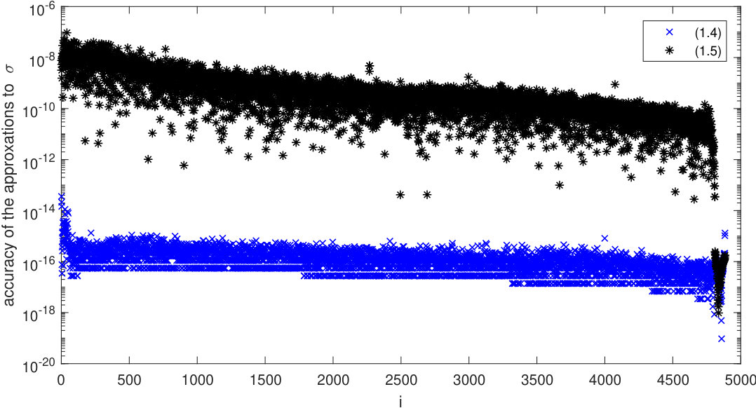 Figure 1
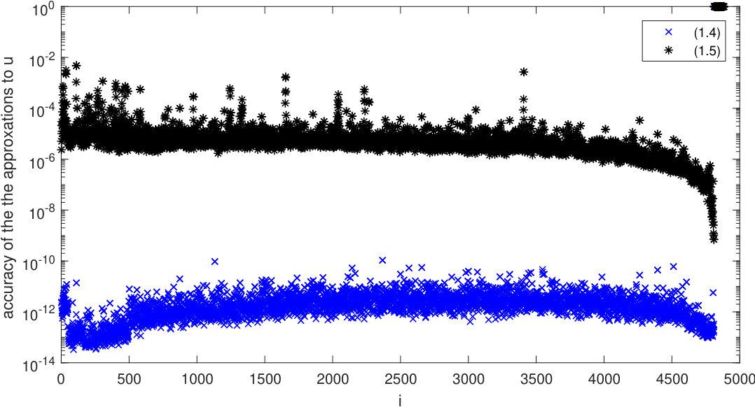 Figure 2
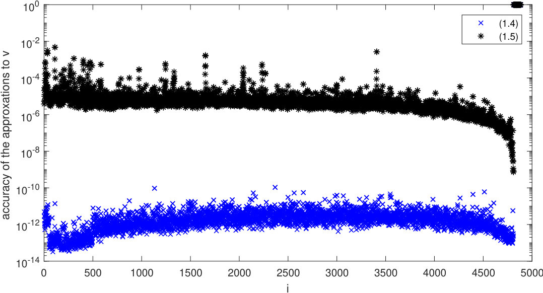 Figure 3
 Figure 4
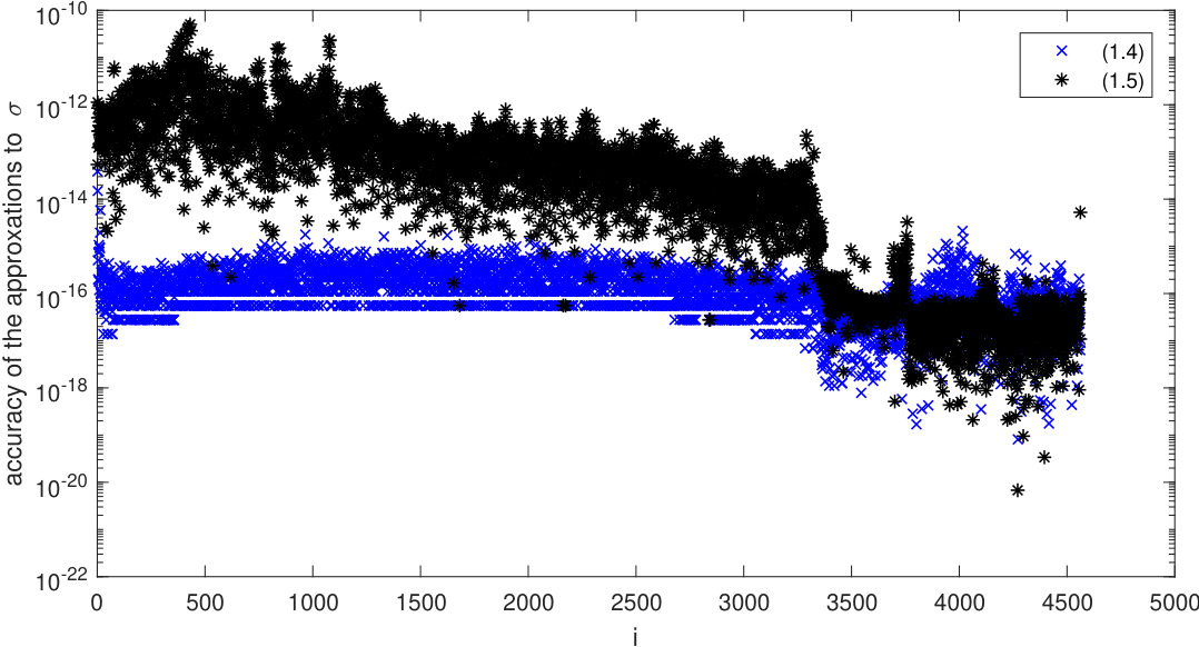 Figure 5
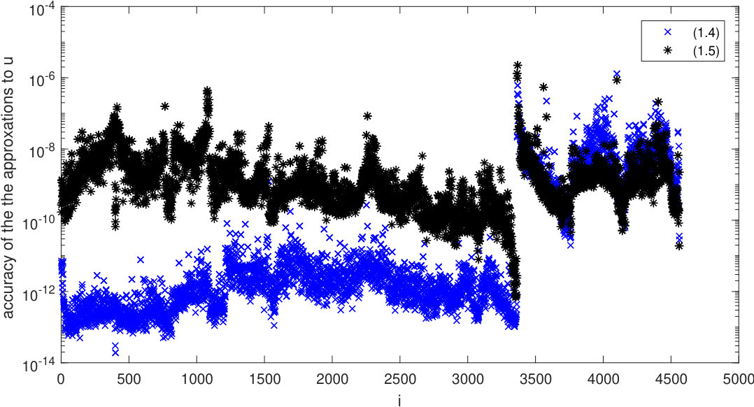 Figure 6
 Figure 7
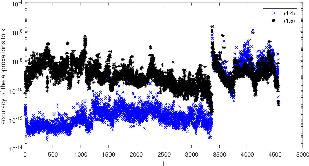 Figure 8
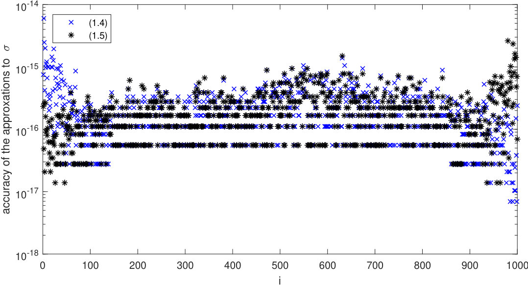 Figure 9
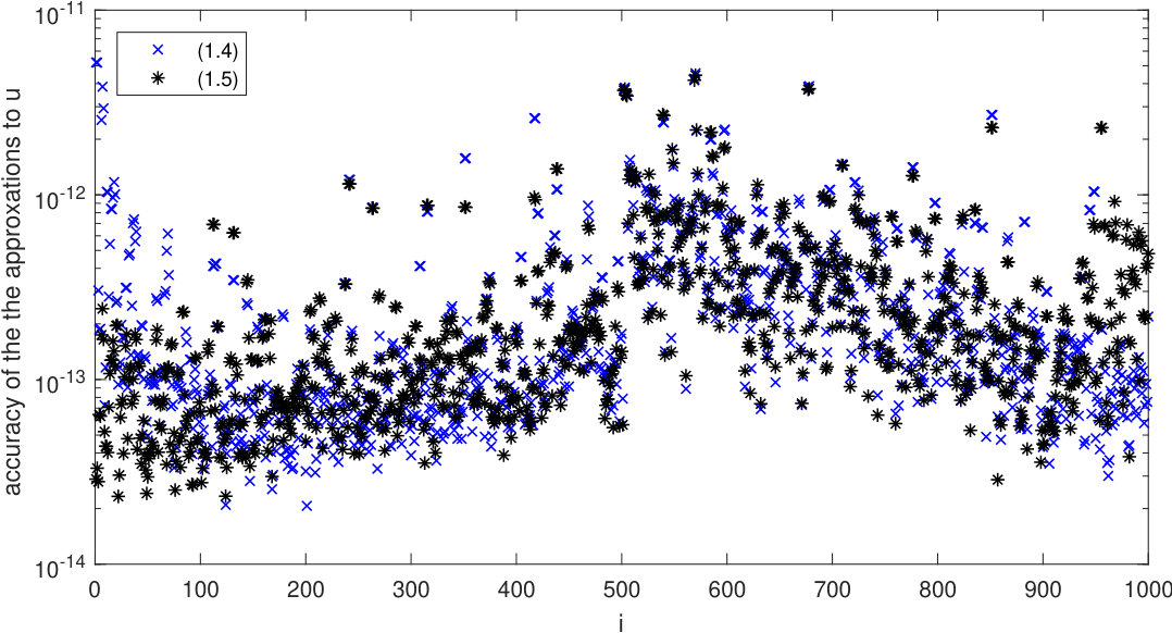 Figure 10
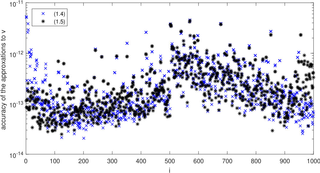 Figure 11
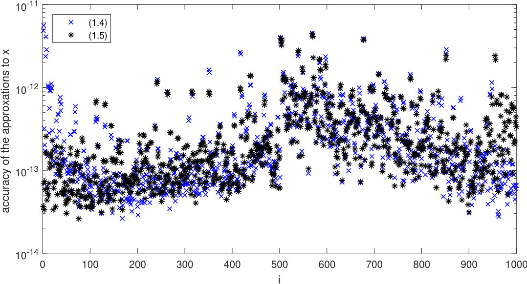 Figure 12
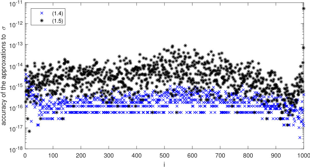 Figure 13
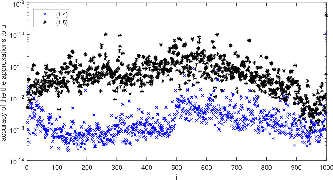 Figure 14
 Figure 15
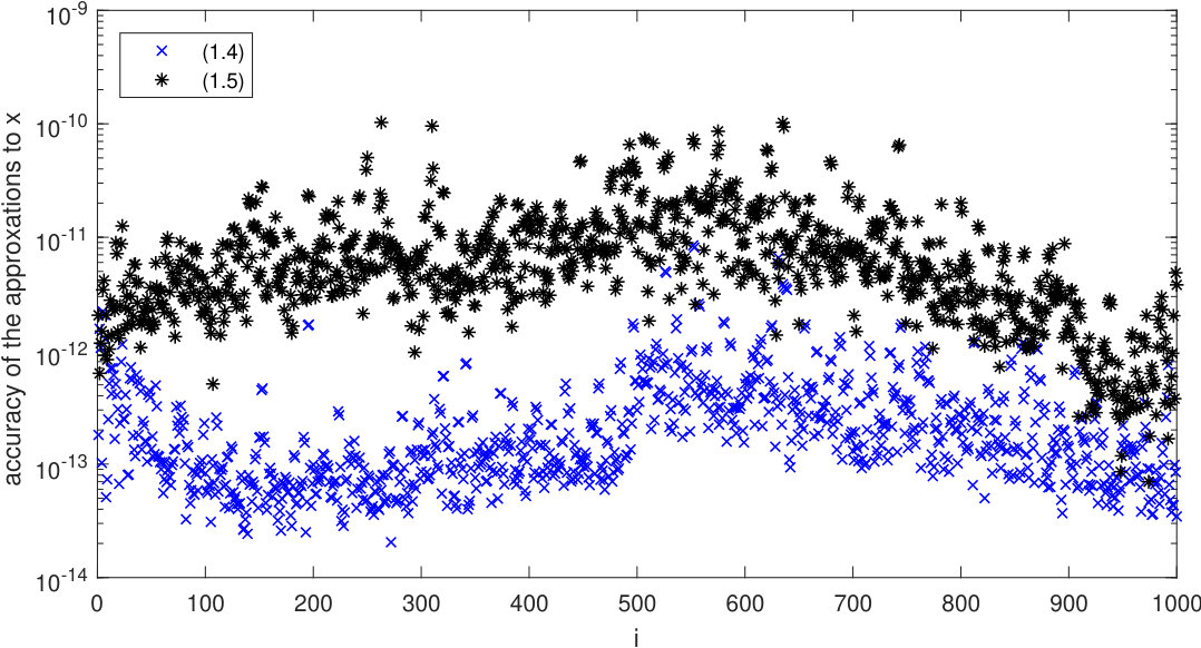 Figure 16
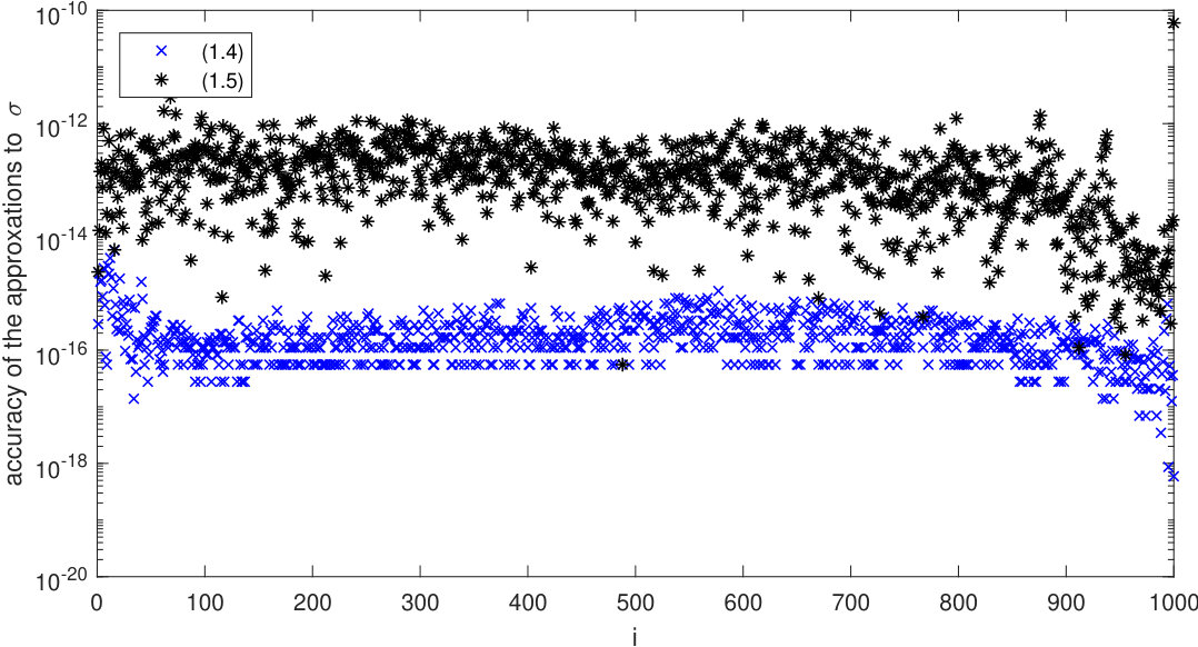 Figure 17
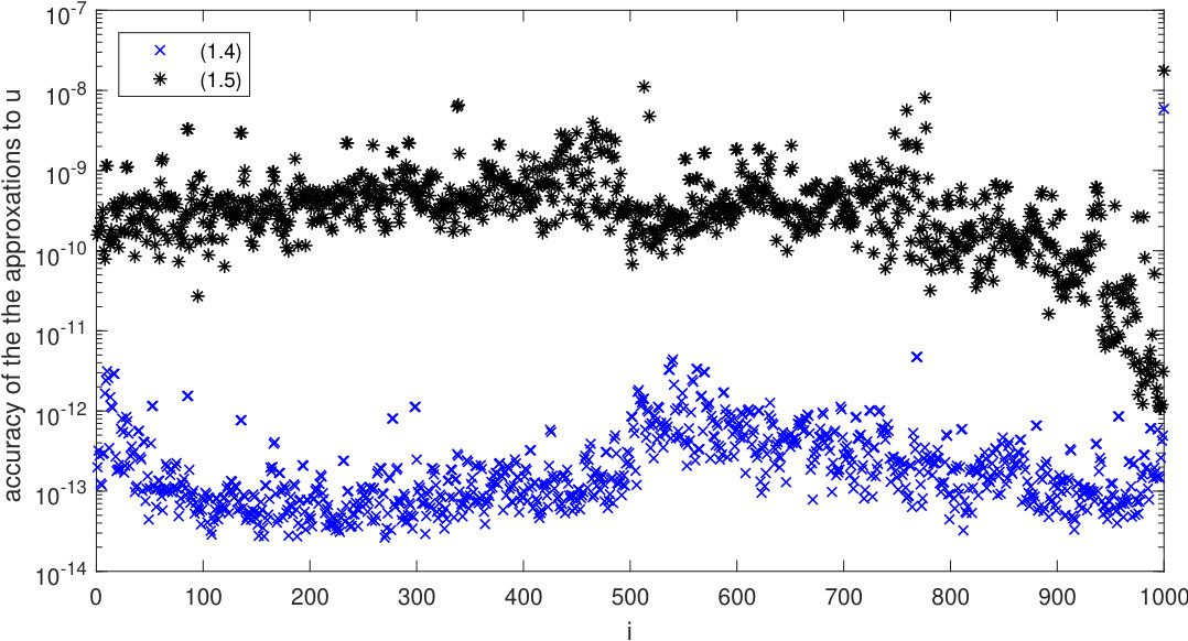 Figure 18
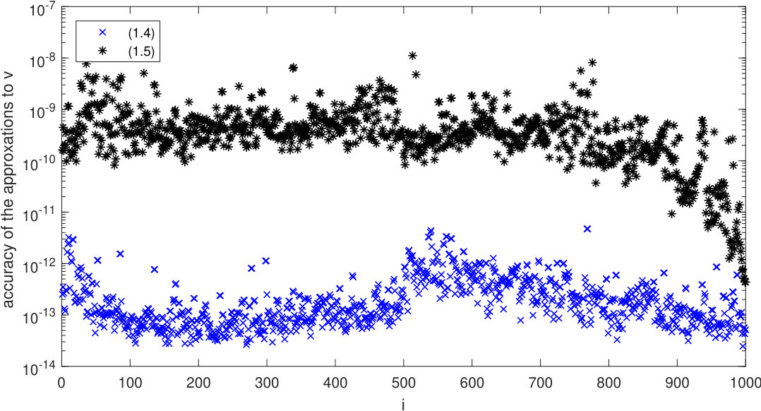 Figure 19
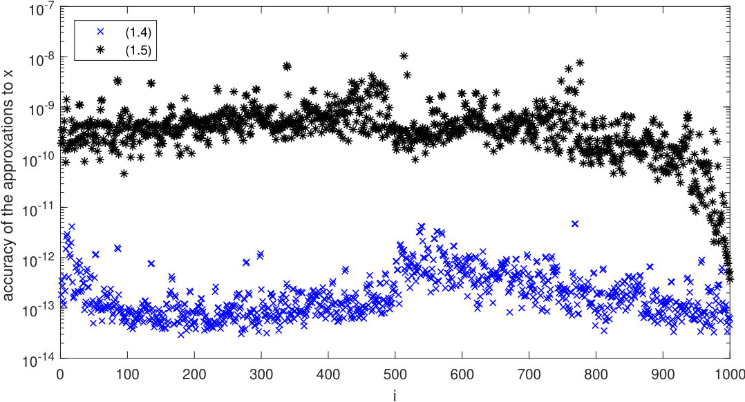 Figure 20
| Problem | |||||||
|---|---|---|---|---|---|---|---|
| 1a | |||||||
| 1b | |||||||
| 1c |
| Problem | ||||||
|---|---|---|---|---|---|---|
| 2a (3elt) | ||||||
| 2b (delan12) | ||||||
| 2c (viscopl1) | ||||||
| 2d (cavity16) | ||||||
| 2e (gemat11) | ||||||
| 2f (bcsstk16) |
| Problem | better | better | better | better | ||||
|---|---|---|---|---|---|---|---|---|
| () | () | () | () | |||||
| 2a | ||||||||
| 2b | ||||||||
| 2c | ||||||||
| 2d | ||||||||
| 2e | ||||||||
| 2f | ||||||||
Peer Reviews
No public reviews on file for this paper yet. If you reviewed it on a platform where reviews are public (OpenReview, ICLR, NeurIPS, ICML), you can paste yours below so the community can read it here.
Videos
No videos yet. Explain this paper in a talk, walkthrough, or lecture? Add one.
∎
11institutetext: Jinzhi Huang 22institutetext: Department of Mathematical Sciences, Tsinghua University, 100084 Beijing, China
22email: [email protected] 33institutetext: Zhongxiao Jia 44institutetext: Corresponding author. Department of Mathematical Sciences, Tsinghua University, 100084 Beijing, China
44email: [email protected]
On choices of formulations of computing
the generalized singular value decomposition of a large matrix pair ††thanks: Supported by the National Natural Science Foundation of China (No.11771249).
Jinzhi Huang
Zhongxiao Jia
Abstract
For the computation of the generalized singular value decomposition (GSVD) of a large matrix pair of full column rank, the GSVD is commonly formulated as two mathematically equivalent generalized eigenvalue problems, so that a generalized eigensolver can be applied to one of them and the desired GSVD components are then recovered from the computed generalized eigenpairs. Our concern in this paper is, in finite precision arithmetic, which generalized eigenvalue formulation is numerically preferable to compute the desired GSVD components more accurately. We make a detailed perturbation analysis on the two formulations and show how to make a suitable choice between them. Numerical experiments illustrate the results obtained.
Keywords:
Generalized singular value decomposition generalized singular value generalized singular vector generalized eigenpair eigensolver perturbation analysis condition number
MSC:
65F15 65F35 15A12 15A18 15A42
1 Introduction
The generalized singular value decomposition (GSVD) of a matrix pair was first introduced by van Loan van1976generalizing and then developed by Paige and Saunders paige1981towards . It has become a standard decomposition and an important computational tool golub2012matrix , and has been extensively used in a wide range of contexts, e.g., solutions of discrete linear ill-posed problems hansen1998rank , weighted or generalized least squares problems bjorck1996numerical , information retrieval howland2003structure , linear discriminant analysis park2005relationship , and many others betcke2008generalized ; chu1987singular ; golub2012matrix ; kaagstrom1984generalized ; vanhuffel .
Let () and () be large and possibly sparse matrices of full column rank, i.e., . The GSVD of is
[TABLE]
where is nonsingular, and are orthonormal, and the positive numbers and satisfy , . We call such a GSVD component of with the generalized singular value , the left generalized singular vectors and , and the right generalized singular vector , . Denote the generalized singular value matrix of by
[TABLE]
Throughout this paper, we also refer to a scalar pair as a generalized singular value of . Particularly, we will denote by and the largest and smallest generalized singular values of , respectively. Obviously, the generalized singular values of the pair are , the reciprocals of those of , and their generalized singular vectors are the same as those of .
For a prescribed target , assume that the generalized singular values of are labeled by
[TABLE]
Specifically, if we are interested in the smallest generalized singular values of and/or the associated left and right generalized singular vectors, we assume in (1.3), so that the generalized singular values are labeled in increasing order; if we are interested in the largest generalized singular values of and/or the corresponding generalized singular vectors, we assume in (1.3), so that the generalized singular values are labeled in decreasing order. More generally, once is bigger than the largest generalized singular value, the generalized singular values closest to are the largest ones of . In these two cases, the GSVD components are called the extreme (smallest or largest) GSVD components of . Otherwise they are called interior GSVD components of if the given is inside the spectrum of the generalized singular values of . We will abbreviate any one of the desired GSVD components as or with the subscripts dropped.
For a large and possibly sparse matrix pair , one kind of approach to compute the desired GSVD components works on the pair directly. Zha zha1996 proposes a joint bidiagonalization method to compute the extreme generalized singular values and the associated generalized singular vectors , which is a generalization of Lanczos bidiagonalization type methods jia2003implicitly ; jia2010 for computing a partial ordinary SVD of when . A main bottleneck of this method is that a large-scale least squares problem with the coefficient matrix must be solved at each step of the joint bidiagonalization. Jia and Yang jiayang2018 has made a further analysis on this method and its variant, and provided more theoretical supports for its rationale.
For the computation of GSVD, a natural approach is to apply a generalized eigensolver to the mathematically equivalent generalized eigenvalue problem of the cross product matrix pair to compute the corresponding eigenpairs and then recover the desired GSVD components from the computed eigenpairs. However, because of the squaring of the generalized singular values of , for small, the eigenvalues of are much smaller. As a consequence, the smallest generalized singular values may be recovered much less accurately and even may have no accuracy jia2006 . Therefore, we will not consider such a formulation in this paper.
Another kind of commonly used approach formulates the GSVD as a generalized eigenvalue problem hochstenbach2009jacobi , where the Jacobi-Davidson method hochstenbach2004 for the ordinary SVD problem has been adapted to a mathematically equivalent formulation of the GSVD so that a suitable generalized eigensolver parlett1998symmetric ; saad2011numerical ; stewart2001matrix can be used. The approach then recovers the desired GSVD components. Concretely, the two formulations proposed in hochstenbach2009jacobi transform the GSVD into the generalized eigenvalue problem of the augmented definite matrix pair
[TABLE]
or the augmented definite matrix pair
[TABLE]
We will give detailed relationships between the GSVD of and the generalized eigenpairs of and in the next section. One then applies a generalized eigensolver to either of them, computes the corresponding generalized eigenpairs, and recovers the desired GSVD components from those computed generalized eigenpairs.
As will be clear next section, the nonzero eigenvalues of and are and , , respectively. Therefore, the largest or interior generalized singular values of become the largest or interior eigenvalues of , and the smallest or interior generalized singular values are the largest and interior eigenvalues of . In principle, we may use a number of projection methods, e.g., Lanczos type methods, to compute the extreme GSVD components via solving the generalized eigenvalue problem of or . For a unified account of projection algorithms, we refer to baiedit2000 . For the computation of interior GSVD components of , we may employ the Jacobi-Davidson type method proposed in hochstenbach2009jacobi , referred as JDGSVD, where at each step a linear system, i.e., the correction equation, is solved iteratively and its approximate solution is used to expand the current searching subspaces. The JDGSVD method deals with the generalized eigenvalue problem of (1.4) or (1.5), computes some specific generalized eigenpairs, and recovers the desired GSVD components from the converged generalized eigenpairs.
As far as numerical computations are concerned, an important question arises naturally: which of the mathematically equivalent formulations (1.4) and (1.5) is numerically preferable, so that the desired GSVD components can be computed more accurately? In this paper, rather than propose or develop any numerical algorithm for computing the desired GSVD components, we focus on this question carefully, give a deterministic answer to it, and suggest a definitive choice. We first make a sensitivity analysis on the generalized eigenpairs of (1.4) and (1.5). Based on the results to be obtained, we establish accuracy estimates for the approximate generalized singular values and the left and right generalized singular vectors that are recovered from the approximate generalized eigenpairs obtained. Then by comparing the accuracy of the approximate GSVD components recovered from the approximate generalized eigenpairs of (1.4) and (1.5), we make a correct choice between these two formulations.
This paper is organized as follows. In Section 2 we make a sensitivity analysis on the generalized eigenvalue problems of the structured matrix pairs and , respectively, and give error bounds for the generalized singular values and the generalized eigenvectors of and . In Section 3 we carry out a sensitivity analysis on the approximate generalized singular vectors that are recovered from the approximate generalized eigenpairs of and . Based on the results and analysis, we conclude that (1.5) is preferable to compute the GSVD more accurately when is well conditioned and is ill conditioned, and (1.4) is preferable when is ill conditioned and is well conditioned. In Section 4 we propose a few practical choice strategies on (1.4) and (1.5). In Section 5 we report the numerical experiments. We conclude the paper in Section 6.
Throughout this paper, denote by the 2-norm of a vector or matrix and the condition number of a matrix with and being the largest and smallest singular values of , respectively, and by the transpose of . Denote by the identity matrix of order , by and the zero matrices of order and , respectively. The subscripts are omitted when there is no confusion. We also denote by the column space or range of . For brevity of our analysis and results, without loss of generality, we suppose that and are comparable in size and, furthermore, and have already been scaled so that their 2-norms are of , that is, roughly, meaning that and roughly and the conditioning of and is reflected by and , respectively.
2 Perturbation analysis of generalized eigenvalue problems
and the accuracy of generalized singular values
The generalized eigendecompositions of the matrix pairs and are closely related to the GSVD of in the following way, which is straightforward to verify.
Lemma 2.1**.**
Let the GSVD of be defined by (1.1) with the generalized singular values defined by (1.2). Let and be such that and are orthogonal. Then the matrix pairs and defined by (1.4) and (1.5) have the generalized eigendecompositions
[TABLE]
respectively, where
[TABLE]
with , and
[TABLE]
with and . Moreover, the columns of the eigenvector matrices and are - and -orthonormal, respectively, i.e.,
[TABLE]
Lemma 2.1 illustrates that the GSVD component of corresponds to the generalized eigenpair
[TABLE]
of the augmented matrix pair with the eigenvector satisfying and and the generalized eigenpair
[TABLE]
of the augmented matrix pair with the eigenvector satisfying and . Therefore, the GSVD of is mathematically equivalent to the generalized eigendecompositions (1.4) and (1.5). In order to obtain some GSVD components , one can compute the corresponding generalized eigenpairs of or of by applying a generalized eigensolver to (1.4) or (1.5), and then recovers the desired GSVD components.
However, in numerical computations, we can obtain only approximate eigenpairs of (1.4) and (1.5), and thus recover only approximate GSVD components of . As a result, when numerically backward stable eigensolvers solve the generalized eigenvalue problems of (1.4) and (1.5) with the computed eigenpairs whose residuals have about the same size, a natural and central concern is: which of the computed eigenpairs of (1.4) and (1.5) will yield more accurate approximations to the desired GSVD components of , that is, which of (1.4) and (1.5) is numerically preferable to compute the GSVD components more accurately?
To this end, we need to carefully estimate the accuracy of the computed eigenpairs and that of the recovered GSVD components. Given a backward stable generalized eigensolver applied to (1.4) and (1.5), let and be the computed approximations to and , respectively. Then and are the exact eigenpairs of some perturbed matrix pairs
[TABLE]
respectively, where the perturbations satisfy
[TABLE]
for small. In applications, we typically have or with being the machine precision baiedit2000 ; golub2012matrix ; parlett1998symmetric ; saad2011numerical ; stewart2001matrix . Here in (2.7), to distinguish from the exact augmented matrices defined in (1.4) and (1.5), we have used the bold letters to denote the perturbed matrices. Notice that the assumption made in Section 1 means , and . Therefore, the perturbations in (2.8) satisfy
[TABLE]
In what follows, we will analyze how accurate the computed eigenpairs and are for a given small .
2.1 The accuracy of generalized singular values
Stewart and Sun in the monograph stewart1990matrix use a chordal metric to measure the distance between the approximate and exact eigenvalues of a regular matrix pair. Let and be the eigenvalues of and . Then the chordal distance between them is
[TABLE]
We present the following results.
Theorem 2.2**.**
Let and be simple eigenpairs of and , respectively, and their approximations and be the exact eigenpairs of the perturbed matrix pairs and , respectively, with the perturbations satisfying (2.8). Assume that the approximate eigenvectors and are decomposed in the unnormalized form of and with and . Then the following error bounds hold:
[TABLE]
where and .
Proof.
By the fact that and , we have and . Applying these two expressions to (2.10), we obtain
[TABLE]
By and , the nominator in the above equality satisfies
[TABLE]
applying which to (2.13) gives rise to
[TABLE]
Notice from with satisfying and that and . Moreover, it has with . Applying these facts to the above inequality gives (2.11).
Replacing , , , and with , , , and , respectively, in (2.11), and exploiting the invariance of the chordal distance under reciprocal, i.e.,
[TABLE]
we obtain (2.12). ∎
Obviously, it can be seen from the proof that (2.11) and (2.12) are independent of scalings of , and , . Therefore, our assumption in the theorem on the unnormalized decomposition form of and is without loss of generality and is only for brevity of the presentation.
For the scalars and in (2.11) and (2.12), we claim that
[TABLE]
for a sufficiently small in (2.8). To show this precisely, without loss of generality, we assume that the approximate eigenvectors of and of are scaled such that and . Moreover, let the generalized eigenvalue and eigenvector matrices of and defined by (2.1) be partitioned as
[TABLE]
Relation (2.4) shows , i.e., the columns of form a basis of , and indicates that we can write for some . By (2.24) to be proved later, we have
[TABLE]
with and being the eigenvalues of other than . If in (2.8) is sufficiently small such that , then from (2.16) we obtain an explicit bound for :
[TABLE]
In an analogous manner, we can obtain .
It is worthwhile to point out that some first order expansions are derived for for a general regular matrix pair in (stewart1990matrix, , p.291-4) but the constants in the second order smaller terms are unknown. The proofs of bounds (2.11) and (2.12) have no special requirement on the matrix pairs and thus are directly applicable to a general regular matrix pair by replacing the transpose by the conjugate transpose and the scalars in the denominators by their absolute values. In comparison with those results in (stewart1990matrix, , p.291-4), however, our bounds contain explicit second order smaller terms since we have obtained the explicit bounds for and .
Exploiting and in Theorem 2.2, and keeping (2.14) in mind, we can present the following results.
Theorem 2.3**.**
Let and be the eigenpairs of and corresponding to the GSVD component of . Assume that their approximations and are the generalized eigenpairs of the perturbed and , respectively, where the perturbations satisfy (2.9). If is sufficiently small, the following error estimates hold:
[TABLE]
where and .
Proof.
It suffices to prove (2.17), and the proof of (2.18) is similar. From Lemma 2.1, notice that the eigenvector of satisfies and . From , and , we have
[TABLE]
Applying this and (2.14) to (2.11) yields (2.17). ∎
Notice from (2.9) that the perturbation terms in the right hand sides of both (2.17) and (2.18) are no more than the same . Theorem 2.3 illustrates that the accuracy of the approximate generalized singular value and that of are determined by and , and by and , respectively. Apparently, a large could severely impair the accuracy of both and . Fortunately, the following bounds show that must be modest under some mild conditions.
Lemma 2.4**.**
Let be the right generalized singular vector matrix of as defined in (1.1) and be an arbitrary column of . Then
[TABLE]
where the superscript denotes the Moore-Penrose generalized inverse of a matrix, and
[TABLE]
Proof.
The bounds in (2.19) and the upper bound for in (2.20) are from Theorem 2.3 of hansen1989regularization . Note that is a column of . Then the lower bound for in (2.20) follows from the fact that
[TABLE]
Lemma 2.4 indicates that, provided that one of and is well conditioned, must be modest. In applications, to our best knowledge, there seems no case that both and are simultaneously ill conditioned. Therefore, without loss of generality, we will assume that at least one of and is well conditioned. Then we have . Under this assumption, the stacked matrix must be well conditioned, too (stewart1990matrix, , Theorem 4.4).
Moreover, Theorem 2.4 of hansen1989regularization shows that provided is well conditioned, the singular values of and those of behave like and , correspondingly: the ratios of the singular values of and (resp. those of the singular values of and ), when labeled by the same order, are bounded from below and above by \big{\|}\begin{bmatrix}\begin{smallmatrix}A\\ B\end{smallmatrix}\end{bmatrix}^{\dagger}\big{\|}^{-1} and \big{\|}\begin{bmatrix}\begin{smallmatrix}A\\ B\end{smallmatrix}\end{bmatrix}\big{\|}, respectively. As a consequence, it is straightforward to justify the following basic properties, which will play a vital role in analyzing the results in this paper.
Property 2.5**.**
Assume that at least one of and is well conditioned.
- •
If both and are well conditioned, no and are small. In this case, all the generalized singular values of are neither large nor small.
- •
If or is ill conditioned, there must be some small or , that is, some generalized singular values must be small or large. Moreover, the small generalized singular values for ill conditioned and the large for ill conditioned.
- •
If is ill conditioned and is well conditioned, all the cannot be large but some of them are small; if is well conditioned and is ill conditioned, all the cannot be small but some of them are large.
Notice that and, . We have
[TABLE]
Therefore, it follows from (2.20) that
[TABLE]
This, together with the assumption , shows that the lower and upper bounds are roughly and 3, respectively, and the ratio is thus very modest. When at least one of and is well conditioned, it is clear that the numerators and in the constants in front of the perturbation terms in bounds (2.17) and (2.18) are not only modest but also very comparable in size. However, it is worthwhile to remind that the lower and upper bounds in (2.21) shows that the ratio is always modest, independent of the conditioning of and . Furthermore, relation (2.21) shows that it is the denominators and that decide the size of the constants in front of the perturbation terms in bounds (2.17) and (2.18). As a consequence, in terms of Theorem 2.3 and Property 2.5, we can draw the following conclusions for the accurate computation of :
- •
For and well conditioned, both (1.4) and (1.5) work well.
- •
If is well conditioned but is ill conditioned, (1.5) is preferable to (1.4).
- •
If is ill conditioned but is well conditioned, (1.4) is better than (1.5).
2.2 The accuracy of generalized eigenvectors
In terms of the angles between the approximate and exact eigenvectors, we present the following accuracy estimates for the approximate eigenvectors of the symmetric definite matrix pairs in (1.4) and (1.5).
Theorem 2.6**.**
With the notations of Theorem 2.2, the following bounds hold:
[TABLE]
where the are the eigenvalues of other than , and the are the eigenvalues of other than .
Proof.
By definition, we have with for some and the matrix defined as in (2.15). By a simple manipulation, we obtain
[TABLE]
Premultiplying both hand sides of the above relation, and noticing from (2.15) and (2.4) that , and , , we obtain
[TABLE]
Taking -norms on both hand sides in the above equality and exploiting
[TABLE]
with being the eigenvalues of other than leads to
[TABLE]
By definition, the sine of the angle between and satisfies
[TABLE]
Substituting and (2.24) into (2.25) yields
[TABLE]
Notice that is positive definite and satisfies . We have
[TABLE]
applying which to (2.26) gives (2.22).
Following the same derivation, we obtain
[TABLE]
with being eigenvalues of other than , i.e., (2.23) holds. ∎
Theorem 2.6 gives accuracy estimates for the approximate eigenvectors of the matrix pairs and . It presents the results in the form of the structured matrix pairs and their eigenvalues. For our use in the GSVD context, substituting the definitions of and in (1.4) and (1.5) as well as their eigenvectors in (2.2) and (2.3) into Theorem 2.6, we can express the results more clearly in terms of the generalized singular values of and the matrices and themselves.
Theorem 2.7**.**
With the notations of Theorem 2.3, the following results hold:
[TABLE]
where the are the generalized singular values of other than .
Proof.
Since the eigenvalues of are and zeros, we have
[TABLE]
where the are the generalized singular values of other than .
On the other hand, by definition (1.4) of , we have
[TABLE]
Applying (2.29) and (2.30) to (2.22), we obtain (2.27).
Notice that the eigenvalues of are and zeros. Following the same derivations as above, we obtain
[TABLE]
which proves (2.28). ∎
Denote and with and . Assume that in (2.9) is sufficiently small. Then from (2.10) and (2.17)–(2.18), we have and . For any generalized singular value of , it is straightforward to obtain
[TABLE]
and
[TABLE]
As a consequence, it holds that
[TABLE]
For the minima in the right-hand sides of (2.31) and (2.32), we have the following result.
Theorem 2.8**.**
Denote and with being the generalized singular values of other than . Then
[TABLE]
To prove this theorem, we need the following lemma.
Lemma 2.9**.**
Define and for . Then
[TABLE]
Proof.
We classify nonnegative as three subintervals:
- •
if , then , and
- •
if , then , and
- •
if , then , and
Summarizing the above establishes (2.34). ∎
Proof of Theorem 2.8.
Denote by and the generalized singular values of that minimize and over all the generalized singular values of other than , respectively. Then and can be written as
[TABLE]
where the functions and are defined by Lemma 2.9. Therefore, the ratio in (2.33) is
[TABLE]
By the definitions of and , we have
[TABLE]
Combining (2.35) with (2.34), we obtain
[TABLE]
which completes the proof. ∎
Theorem 2.8, together with (2.31) and (2.32), means that the factors and in (2.27) and (2.28) have approximately the same size and both are approximately the relative separation of the desired from the other generalized singular values of . The bigger they are, i.e., the better the desired generalized singular value is separated from the others, the more accurate the approximate eigenvectors of (1.4) and (1.5) are.
For a given , (2.9) tells us that and in (2.27) and (2.28) are approximately equal. Therefore, Theorems 2.7–2.8 and , show that which of and is more accurate critically depends on the sizes of and . Keep in mind that means that and . Combining these results with Property 2.5, for a proper choice of (1.4) and (1.5) for computing eigenvectors more accurately, we can draw the following conclusions with the arguments included.
- •
If and have roughly the same conditioning and both are well conditioned, then cannot be large or small. In this case, both (1.4) and (1.5) are proper formulations of computing the generalized eigenvectors and with similar accuracy.
- •
For ill conditioned and well conditioned, assuming that the are labeled in decreasing order, from Property 2.5, since the pair has large generalized singular values but has no small one, it is known that . Therefore, we have
[TABLE]
for any . Therefore, (1.5) is preferable to compute any eigenvector more accurately.
- •
For well conditioned and ill conditioned, from Property 2.5, since some generalized singular values of are small but none is large, it is known that . Therefore, we always have
[TABLE]
for any . This means that (1.4) is preferable to compute any eigenvector more accurately.
Finally, we notice from Theorem 2.7 that or may have no accuracy at all whenever or is as large as , even though a backward stable generalized eigensolver is applied to (1.4) or (1.5) and backward errors are . For a large matrix pair , iterative projection methods are used to compute some specific GSVD components and stopping criteria are typically , so that backward errors are . In this case, or may have no accuracy provided that or is as large as .
3 The accuracy of generalized singular vectors
After applying a generalized eigensolver to the matrix pair or , the computed eigenvalue or provides an approximation to the desired generalized singular value directly. However, the situation is complicated and more involved for generalized singular vectors since the generalized eigenvector
[TABLE]
defined by (2.5) or (2.6) is a stack of the normalized left generalized singular vector or and the scaled right generalized singular vector
[TABLE]
We must recover approximations to the generalized singular vectors from a computed approximate eigenvector or . For the GSVD components of , our next task is to determine which of and delivers more accurate approximations to and when the perturbations and in (2.7) approximately have the same size in norm.
For (1.4), after a generalized eigensolver is run, we write the converged approximate eigenvector as with normalized to have unit length and . Then and provide approximations to the left generalized singular vector and the right generalized singular vector , respectively, with the computed . As for the left generalized singular vector , since , it is natural to take the unit length as its approximation.
Analogously, for (1.5), we partition such that is normalized to have unit length, , and that and are approximations to the left generalized singular vector and the right generalized singular vector , respectively, where the computed . Since , we take the unit length as an approximation to .
Previously we have derived error estimates on and for the approximate eigenvectors and . Next we exploit them to estimate the accuracy of the approximate generalized singular vectors and recovered in the manner described above. To this end, we prove the following lemma, which is a generalization of Theorem 2.3 in jia2003implicitly .
Lemma 3.1**.**
Assume that and are arbitrary nonzero vectors, and let and be approximations to them, respectively. Then
[TABLE]
Moreover, it holds that
[TABLE]
where
Proof.
By definition, the sine of the angle between two vectors and satisfies
[TABLE]
A similar relation holds with and replaced by and , respectively. Combining these two relations with the inequality
[TABLE]
proves (3.2). From (3.2), taking the smaller one of and yields (3.3). It is also straightforward to obtain
[TABLE]
Combining the above two inequalities gives rise to (3.4). ∎
Taking , and , , bound (3.3) illustrates that at least one of the recovered approximate generalized singular vectors and is as accurate as . Since , bound (3.4) indicates that if then both and have the same accuracy as . But bound (3.4) also states that if is very small or large relative to then one of and may have considerably poorer accuracy than due to the large factor . Fortunately, a very small is unlikely to happen as is always modest under the assumption that at least one of and is well conditioned, implying that cannot be small as . On the other hand, when the largest GSVD components of are required, a large definitely appears if is ill conditioned since behaves like the singular values of and is small, as Property 2.5 shows.
Precisely, based on Lemma 3.1, we can derive quantitative accuracy estimates for the recovered approximate generalized singular vectors, as will be shown below.
Theorem 3.2**.**
The scaled right generalized singular vector , defined in (3.1), of satisfies
[TABLE]
For the approximate generalized singular vectors and recovered from the approximate eigenvector of (1.4), it holds that
[TABLE]
Proof.
From and we have
[TABLE]
which shows (3.5).
Take , in Lemma 3.1. Neglecting the first term in the left hand side of (3.2), we obtain
[TABLE]
which proves (3.6).
Neglecting the second term in the left hand side of (3.2) gives (3.7).
As for , exploiting with and combining (3.6) with , we have
[TABLE]
which proves (3.8). ∎
As , this theorem shows that the recovered approximate generalized singular vector is unconditionally as accurate as , but and are guaranteed to be as accurate as only if is not small. As Property 2.5 indicates, it is the conditioning of that determines the size of : for well conditioned, there is no small , so that the recovered approximate generalized singular vectors are guaranteed to be as accurate as ; for ill conditioned, some must be small so that is large, which correspond to large generalized singular values , so that the associated recovered and may have poorer accuracy than .
In an analogous manner, we can prove the following results.
Theorem 3.3**.**
The scaled right generalized singular vector , defined in (3.1), of satisfies
[TABLE]
For the approximate generalized singular vectors and recovered from the approximate eigenvector of (1.5), it holds that
[TABLE]
The comments on Theorem 3.2 apply to this theorem: is always as accurate as ; and are guaranteed to be as accurate as only if is fairly modest, and they may be considerably poorer than when is large, i.e., when is small. From Property 2.5, it is known that if is well conditioned then no is small but if is ill conditioned then some must be small, which correspond to small generalized singular values .
Recall the previous fundamental conclusions on the accuracy of and , which have been summarized in the near end of Section 2. Substituting the bounds in Theorem 2.7 for and into Theorems 3.2–3.3, we obtain the corresponding error estimates for the approximate generalized singular vectors recovered from the approximate eigenvectors of (1.4) and of (1.5), as summarized below.
Theorem 3.4**.**
The approximate generalized singular vectors , , and recovered from the approximate eigenvector of (1.4) satisfy
[TABLE]
Similarly, the approximate generalized singular vectors , , and recovered from the approximate eigenvector of (1.5) satisfy
[TABLE]
Combining these bounds with the above analysis and the claims in the near end of Section 2, we come to the following conclusions on a proper choice of (1.4) and (1.5) for more accurate computations of generalized singular vectors.
- •
If both and are equally conditioned, i.e, both of them are well conditioned, both (1.4) and (1.5) are suitable choices.
- •
If is well conditioned and is ill conditioned, (1.5) is preferable.
- •
If is ill conditioned and is well conditioned, (1.4) is preferable.
By comparing these conclusions with those in the end of Section 2.1 for accurate computations of generalized singular values, we find out that they exactly coincide. Therefore, we have finally achieved our ultimate goal of making a proper choice of (1.4) and (1.5): the above conclusions apply to more accurate computations of both generalized singular values and generalized singular vectors .
4 Practical choice strategies on
In Sections 2–3 we have made a sensitivity analysis on the generalized singular values and the corresponding generalized singular vectors of , which are computed by solving the generalized eigenvalue problems of (1.4) and (1.5). The results have shown that, in order to compute the desired GSVD components of more accurately, we should make a preferable choice between (1.4) and (1.5). To be practical in computations, this requires to estimate the condition numbers of and efficiently and reliably.
For and large-scale, note that we do not need to estimate and accurately, and rough estimates are enough. Taking as an example, we describe three approaches to estimate roughly. As and , estimating is equivalent to estimating .
The first approach: if is large-scale with special structures such that the matrix-vector multiplication with the matrix can be implemented at affordable extra cost, then one can perform a -step symmetric Lanczos method baiedit2000 ; parlett1998symmetric on and take the square root of the largest approximate eigenvalue as a reasonable estimate of . In the algorithm, what we need is to form and compute its Cholesky factorization, which is used to solve lower and upper triangular linear systems at each step of the Lanczos method. The largest eigenvalue and possibly the smallest eigenvalue of can be well approximated from below and above by the largest and smallest ones of the symmetric tridiagonal matrices generated by the Lanczos process, respectively parlett1998symmetric . With , this method outputs a lower bound for . Since we do not need to estimate accurately and the Lanczos method generally converges quickly for computing the largest and smallest eigenvalues, we suggest to take a small in practice.
The second approach: when is a general large matrix, it is unaffordable to apply . Avron, Druinsky and Toledo avron2013spectral propose a randomized Krylov subspace method to estimate the condition number of a matrix . In their method, a consistent linear least squares problem, whose solution is generated randomly, is solved iteratively by the LSQR algorithm bjorck1996numerical , and the smallest singular value of is estimated by with being the error of the approximate solution and the exact one. We refer the reader to avron2013spectral for details.
The third approach: as an alternative of the second approach, one can also perform a -step Lanczos bidiagonalization type method on and take the largest and smallest singular values of the resulting small projected matrix as approximations to the largest and smallest singular values of ; see jia2003implicitly ; jia2010 . We then take their ratio as a rough approximation to . Still, we take a small in practice. In this way, we can efficiently estimate .
Having estimated and using one of the above approaches, taking the resulting estimates as replacements of and , and based on the previous results and analysis, one can make a proper choice of (1.4) and (1.5) according to the following strategy.
- •
If , which means that and are equally well conditioned, then both (1.4) and (1.5) are suitable;
- •
If , which means that is worse conditioned than , then (1.5) is adopted;
- •
If , which means that is worse conditioned than , then (1.4) is recommended.
5 Numerical experiments
In this section, we report numerical experiments to confirm our theory. We do not aim to develop any algorithms based on (1.4) and (1.5) in this paper. Rather, we simply apply some existing numerically backward stable algorithms to them and compute their generalized eigendecompositions. In the experiments, we use the QZ algorithm, i.e., the Matlab built-in function eig, for the generalized eigenvalue problems (1.4) and (1.5). For each matrix pair , we recover all the GSVD components and from the computed eigenpairs of the augmented matrix pairs and , respectively, i.e., and , which are obtained by applying eig to (1.4) and (1.5), respectively. The “” GSVD components are computed by applying the Matlab built-in function gsvd to . 111For the right generalized singular vector matrix in (1.1), gsvd outputs in our notation. Hence is recovered by using the Matlab built-in function inv and taken as the transpose of inv().
We compare solution accuracy of the GSVD components based on (1.4) and (1.5), and mainly justify three points: (i) if both and are well conditioned, then both (1.4) and (1.5) are suitable for computing the GSVD of accurately; (ii) if is ill conditioned and is well conditioned, then (1.4) is preferable to compute the GSVD accurately; (iii) if is well conditioned and is ill conditioned, then (1.5) is a better formulation for computing the GSVD accurately. As mentioned in the beginning of section 1, the GSVDs of the matrix pairs and are the same with the generalized singular values being the reciprocals of each other. Under the assumption that at least one of and is well conditioned, we can always take one of them to be well conditioned and the other one well conditioned or ill conditioned. Therefore, for the sake of certainty in the experiments, we always take to be well conditioned but to be well or ill conditioned. In the meantime, we justify Property 2.5.
All the numerical experiments were performed on an Intel (R) Core (TM) i7-7700 CPU 3.60 GHz with 8 GB RAM, 4 cores and 8 threads using the Matlab R2017a with the machine precision under the Microsoft Windows 8 64-bit system.
We measure the accuracy of the computed generalized singular values by their chordal distances from their exact counterparts and measure the accuracy of the computed generalized singular vectors by the sines of the angles between them and their exact counterparts.
Each figure in this section consists of four subfigures: the top left one depicts the accuracy of the computed generalized singular values such that ’s are sorted in descending order; the top right, bottom left and right ones depict the accuracy of the computed right and left generalized singular vectors and , , respectively.
Experiment 5.1**.**
We first test three randomly generated problems. For prescribed constants and , we generate the random sparse matrix and matrix by the Matlab commands
[TABLE]
with the density , and and . The largest singular values of such and are equal to one, i.e., , and their condition numbers are and , respectively. Therefore, by prescribing the values of and , we control the condition numbers and . Table 1 lists the test problems together with their basic properties. Figures 1-3 display the results.
From Table 1 we see that and , confirming Property 2.5 and the third conclusion in the near end of Section 2. We notice that as long as at least one of and is well conditioned, so is the stacked matrix .
For problem 1a, both and are well conditioned. Figure 1 illustrates that both (1.4) and (1.5) yield equally accurate GSVD components of . Apparently, there is no winner between (1.4) and (1.5) for this problem.
For problem 1b, is moderately ill conditioned and is well conditioned. As is observed from Figure 2a, the computed generalized singular values based on (1.4) are generally more accurate than those based on (1.5), or at least as comparably accurate as the latter ones. Figures 2b-2d show that for most of the generalized singular vectors, (1.4) yields significantly more accurate approximations than (1.5) does. Therefore, (1.4) outperforms (1.5) for this problem.
For problem 1c where is quite ill conditioned and is well conditioned, the advantage of (1.4) over (1.5) is very obvious. As is visually illustrated by Figure 3, for all the generalized singular components, (1.4) yields more or even much more accurate approximations than (1.5), and the accuracy is improved by several orders. For this problem, (1.4) definitely wins.
For these three problems, we have observed that for both and well conditioned, two formulations (1.4) and (1.5) based backward stable algorithms deliver equally accurate approximations to the GSVD components of . For the problems where is ill conditioned and is well conditioned, (1.4) can produce more and even much more accurate GSVD components than (1.5). Moreover, with being well conditioned, the worse conditioned is, the more advantageous (1.4) is over (1.5). As is also observed from Figures 1-3, a suitable choice between (1.4) and (1.5) can always guarantee that under the chordal measure all the generalized singular values can be computed with full accuracy, i.e., the level of , which confirms Theorem 2.3 and the analysis followed in Section 2.1.
Experiment 5.2**.**
We test several realistic problems. For each problem, the matrices and are normalized from and , respectively, i.e., and , where is a square matrix from the SuiteSparse Matrix Collection davis2011university and
[TABLE]
is the transpose of the first order derivative operator in dimension one hansen1998rank . Table 2 lists the test problems together with some of their basic properties, where the names inside the brackets are those of the initial matrices , in which “delan12” and “viscopl1” are abbreviations for “delaunay_n12” and “viscoplastic1”, respectively.
We observe from Table 2 that well and roughly, justifying Property 2.5 and the third conclusion in the near end of Section 2.
Table 3 displays some key data that exhibit the advantages of (1.4) over (1.5) when computing the GSVD of more accurately, where denotes the percentages that the computed GSVD components based on (1.4) are more accurate than those based on (1.5), and denotes the average orders of magnitude differences between the accuracy of the computed GSVD components based on (1.4) and the accuracy of those based on (1.5), i.e., for the generalized singular values is defined by
[TABLE]
Apparently, the bigger and are, the more accurate the GSVD components based on (1.4) are than those based on (1.5) on average. and indicate that, on average, there is little difference and these two formulations based backward stable eigensolvers compute the GSVD with similar accuracy.
For these six test problems, we have observed very similar phenomena to the previous experiments. For problems 2a and 2b where both and are equally well conditioned, (1.4) and (1.5) are competitive and there is no obvious winner between them, though (1.5) is slightly better than (1.4). However, we have seen that, for problems 2c-2f, the matrix is increasingly worse conditioned than , the measures and increase and become near to one and bigger, respectively, meaning that more and more GSVD components are computed more and even much more accurately based on (1.4) than on (1.5). Therefore, (1.4) outperforms (1.5) for these four problems.
To illustrate the accuracy visually, we depict the results on problems 2d and 2f in Figures 5 and 5, respectively. For problem 2d, the matrix is well conditioned and is ill conditioned. We can see from Figure 5 that for the largest of the GSVD components, (1.4) outperforms (1.5) substantially, but for the rest smallest ones, the two formulations are competitive as they yield comparably accurate approximations. Particularly, from Figure 5, we also observe a loss of accuracy of the approximate generalized singular vectors around the th GSVD component. This occurs because of very small relative gaps between the corresponding generalized singular values. For problem 2f where is well conditioned and is worse conditioned, (1.4) outperforms (1.5) more substantially and the accuracy improvements illustrated by Figure 5 are tremendous. We observe that for almost all (more than 99%) GSVD components of , (1.4) yields much more accurate approximations than (1.5) does. In addition, we see from Figure 5 that for the several smallest GSVD components, using (1.5) can compute generalized singular values accurately, but the corresponding computed generalized singular vectors have no accuracy at all, while (1.4) works very well. This is not surprising and is in accordance with our comments in the near end of Section 2 by noticing that .
Finally, for all the test problems, we have observed that, with the suitable formulation chosen and under the chordal measure, the generalized singular values are always computed with full accuracy, which justifies Theorem 2.3 and the analysis followed in Section 2.1.
Summarizing all the experiments, we conclude that (i) both (1.4) and (1.5) suit well for problems where both and are well conditioned, (ii) (1.4) is preferable for problems where is ill conditioned and is well conditioned, and (iii) (1.5) is preferable for problems where is well conditioned and is ill conditioned. Therefore, the numerical experiments have fully justified our theory.
6 Conclusions
The GSVD of the matrix pair can be formulated as two mathematically equivalent generalized eigenvalue problems of the matrix pairs defined by (1.4) and (1.5), to which a generalized eigensolver can be applied, and the GSVD components are recovered from the computed generalized eigenpairs. However, in numerical computations, the two formulations may behave very differently for computing the GSVD, and the same generalized eigensolver applied to them may compute GSVD components with quite different accuracy. We have made a detailed sensitivity analysis on the generalized singular values and the generalized singular vectors recovered from the computed eigenpairs by solving the generalized eigenvalue problems of the matrix pairs defined by (1.4) and (1.5), respectively. The results and analysis have shown that (i) both (1.4) and (1.5) are suitable when both and are well conditioned; (ii) (1.4) is preferable when is ill conditioned and is well conditioned; (iii) (1.5) suits better when is well conditioned and is ill conditioned. We have also proposed practical strategies of making a suitable choice between (1.4) and (1.5) in practical computations.
Illuminating numerical experiments have confirmed our theory and supported our choice strategies on (1.4) and (1.5).
The reference list from the paper itself. Each links out to its DOI / PubMed record.
- 1(1) Avron, H., Druinsky, A., Toledo, S.: Spectral condition-number estimation of large sparse matrices. Numer. Linear Algebra Appl. p. e 2235 (2019)
- 2(2) Bai, Z., Demmel, J., Dongrra, J., Ruhe, A., van der Vorst, H.A.: Templates for the Solution of Algebraic Eigenvalue Problems: A Practical Guide. SIAM, Philadelphia (2000)
- 3(3) Betcke, T.: The generalized singular value decomposition and the method of particular solutions. SIAM J. Sci. Comput. 30 , 1278–1295 (2008)
- 4(4) Björck, Å.: Numerical Methods for Least Squares Problems. SIAM, Philadelphia (1996)
- 5(5) Chu, K.W.E.: Singular value and generalized singular value decompositions and the solution of linear matrix equations. Linear Algebra Appl. 88 , 83–98 (1987)
- 6(6) Davis, T.A., Hu, Y.: The University of Florida sparse matrix collection. ACM Trans. Math. Software 38 , 1–25 (2011). Data available online at http://www.cise.ufl.edu/research/sparse/matrices/
- 7(7) Golub, G.H., van Loan, C.F.: Matrix Computations. John Hopkins University Press (2012)
- 8(8) Hansen, P.C.: Regularization, GSVD and truncated GSVD. BIT 29 , 491–504 (1989)