Generalized dilaton-axion models of inflation, de Sitter vacua and spontaneous SUSY breaking in supergravity
Yermek Aldabergenov, Auttakit Chatrabhuti, Sergei V. Ketov

TL;DR
This paper develops unified supergravity models that explain inflation, dark energy, and SUSY breaking using a dilaton-axion field, with viable inflationary parameters and high SUSY breaking scales consistent with observations.
Contribution
It introduces a class of supergravity models with a specific Kähler potential and superpotential that unify inflation, SUSY breaking, and dark energy phenomena.
Findings
Viable inflation occurs for 3 ≤ α ≤ 7.235.
Primordial perturbation amplitude fixes SUSY breaking scale at ~10^{13} GeV.
Axion mass is comparable to inflaton mass for α > 3.
Abstract
We propose the unified models of cosmological inflation, spontaneous SUSY breaking, and the dark energy (de Sitter vacuum) in supergravity with the dilaton-axion chiral superfield in the presence of an vector multiplet with the alternative Fayet-Iliopoulos term. By using the K\"ahler potential as and the superpotential as a sum of a constant and a linear term, we find that viable inflation is possible for where . Observations of the amplitude of primordial scalar perturbations fix the SUSY breaking scale in our models as high as GeV. In the case of the axion gets the tree-level (non-tachyonic) mass comparable to the inflaton mass.
Click any figure to enlarge with its caption.
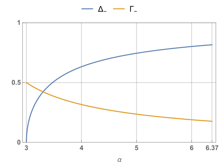 Figure 1
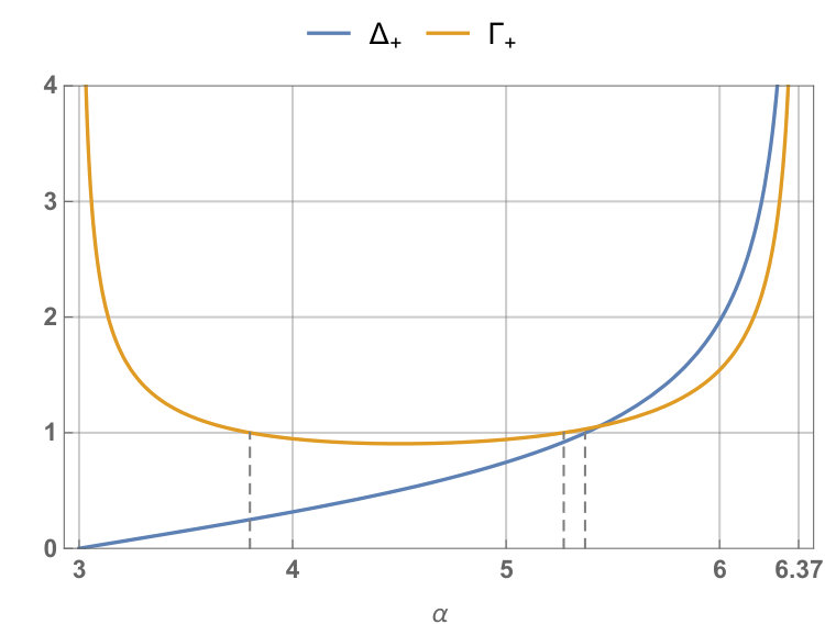 Figure 2
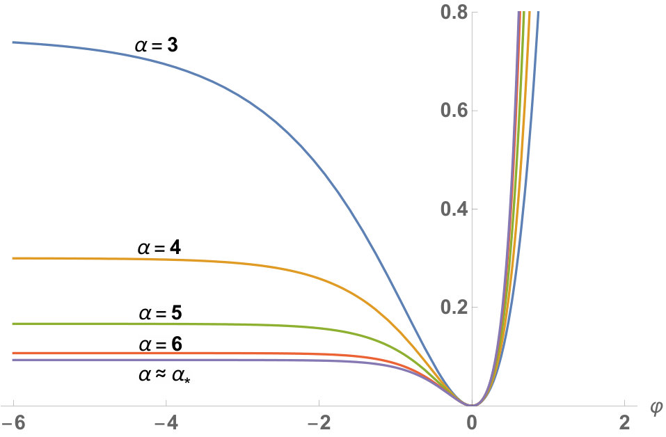 Figure 3
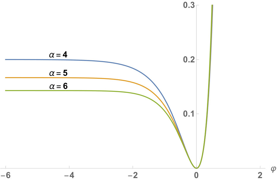 Figure 4
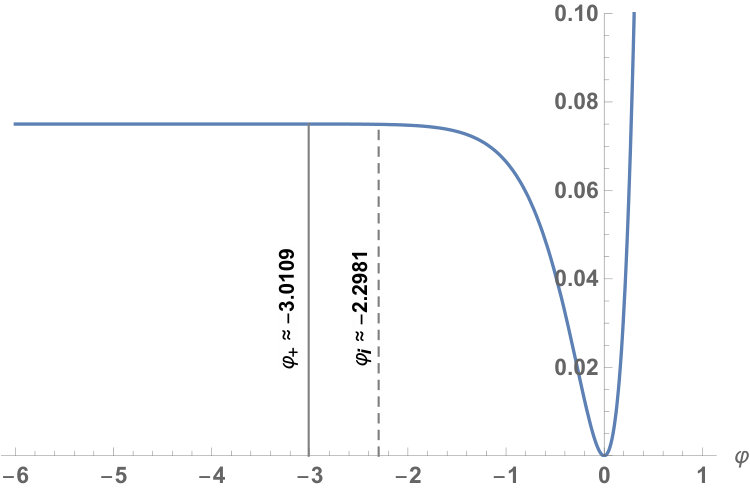 Figure 5
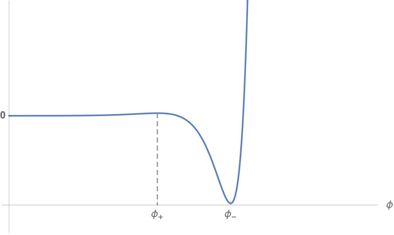 Figure 6
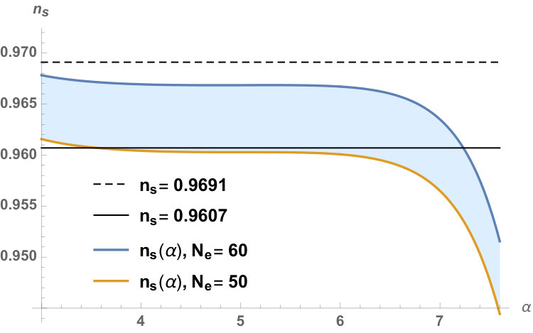 Figure 7
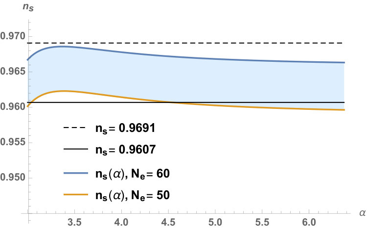 Figure 8
| any | |||||||||
Peer Reviews
No public reviews on file for this paper yet. If you reviewed it on a platform where reviews are public (OpenReview, ICLR, NeurIPS, ICML), you can paste yours below so the community can read it here.
Videos
No videos yet. Explain this paper in a talk, walkthrough, or lecture? Add one.
July 2019 IPMU19-0096
Generalized dilaton-axion models of inflation, de Sitter vacua and spontaneous SUSY breaking in supergravity
Yermek Aldabergenov *a,b,*[email protected], Auttakit Chatrabhuti *a,*[email protected] and Sergei V. Ketov *c,d,e,*[email protected]
a Department of Physics, Faculty of Science, Chulalongkorn University,
Thanon Phayathai, Pathumwan, Bangkok 10330, Thailand
b Institute for Experimental and Theoretical Physics, Al-Farabi Kazakh National University,
71 Al-Farabi Avenue, Almaty 050040, Kazakhstan
c Department of Physics, Tokyo Metropolitan University,
Minami-ohsawa 1-1, Hachioji-shi, Tokyo 192-0397, Japan
d Research School for High Energy Physics, Tomsk Polytechnic University,
30 Lenin Avenue, Tomsk 634050, Russian Federation
e Kavli Institute for the Physics and Mathematics of the Universe (IPMU),
The University of Tokyo, Chiba 277-8568, Japan
Abstract
We propose the unified models of cosmological inflation, spontaneous SUSY breaking, and the dark energy (de Sitter vacuum) in supergravity with the dilaton-axion chiral superfield in the presence of an vector multiplet with the alternative Fayet-Iliopoulos term. By using the Kähler potential as and the superpotential as a sum of a constant and a linear term, we find that viable inflation is possible for where . Observations of the amplitude of primordial scalar perturbations fix the SUSY breaking scale in our models as high as GeV. In the case of the axion gets the tree-level (non-tachyonic) mass comparable to the inflaton mass.
1 Introduction
Supergravity is well motivated as the possible theoretical interface between (a) high-energy physics (well) beyond the Standard Model (SM) of elementary particles, (b) gravity beyond the Concordance (CDM) Cosmological Model, and (c) string theory as the theory of quantum gravity whose low-energy effective action is described by supergravity. A phenomenological description of high energy particle physics and cosmology in supersymmetry (SUSY) and supergravity is known to be non-trivial, though many viable models exist, see e.g., the reviews [1, 2, 3, 4] and the references therein. No signs of SUSY at the Large Hadron Collider (LHC) may hint towards a high scale of SUSY phenomena. At such scales (indirect) cosmological probes of SUSY prevail over (direct) experimental probes at particle colliders. The early Universe is, therefore, the natural place for physical applications of supergravity.
A simultaneous description of cosmological inflation and dark energy (as the positive cosmological constant) in supergravity is another challenge due to the huge difference in the relevant scales and the need of (spontaneous) SUSY breaking. The standard approach in supergravity is based on the use of chiral superfields in four spacetime dimensions with the input given by a Kähler potential and a superpotential . Then the scalar potential and the kinetic terms of the scalar field components are uniquely defined, and the phenomenological model building amounts to choosing both and in order to achieve a viable single-field inflation consistent with the Cosmic Microwave Background (CMB) observations and a de Sitter (dS) vacuum after inflation. There are several problems with that approach. First, the input given by and allows infinitely many choices. Second, it always leads to the multi-scalar framework so that one has to choose the inflaton direction in the field space and suppress the non-inflaton scalars during inflation in order to prevent spoiling of the inflaton slow roll and get enough number of e-foldings. Third, after inflation one has to get the hierarchy between the (high) SUSY breaking scale allowing large masses for the superpartners of the SM particles and the (low) dark energy scale given by the cosmological constant. Getting that hierarchy may require two different mechanisms of spontaneous SUSY breaking.
It is possible to reduce (and minimize) the number of scalars in the inflationary models by employing a massive (irreducible) vector multiplet as the inflaton supermultiplet, instead of a chiral one [5, 6]. The massive vector multiplet has only one (real) physical scalar that can be identified with inflaton, while its fermionic superpartner can be identified with goldstino in the minimalistic setup for inflation in supergraviity (cf. Refs. [7, 8]). To avoid SUSY restoration after inflation in a Minkowski vacuum (it was the drawback of the first supergravity models with inflaton in a vector multiplet), one may either add the hidden sector described by a chiral (Polonyi) superfield as in Refs. [9, 10, 11] or introduce the alternative (new) Fayet-Iliopoulos (FI) terms as in Refs. [12, 13]. 444The alternative FI terms without gauging the R-symmetry were introduced in Refs. [14, 15]. Moreover, one can also combine both approaches and derive the supergravity-based inflationary models with inflaton in a massive vector multiplet in the presence of the FI term, with both F-type and D-type SUSY breaking needed for the hierarchy of scales [16, 17]. In all those cases, the canonical Kähler potential and a linear superpotential for Polonyi superfield were chosen, like the original Polonyi model [18].
Another approach is based on the use of the ”dilaton-axion” superfield by replacing the canonical (free) Kähler potential by the generalized ”no-scale” one as follows [19]:
[TABLE]
The corresponding non-linear sigma-model has the (or ) tangent space of Kähler curvature , and is of particular interest for particle phenomenology because such Kähler potential in the case of arises in generic heterotic string compactifications and allows for the realistic particle model building [19, 20, 21, 22]. Then can be identified with the volume modulus of the compactified manifold in heterotic string theory. It is remarkable that the same Kähler potential with also arises in the modified supergravity after its dualization [23, 24, 25].
It is, however, also known that the case of in Eq. (1) with just a single chiral superfield is not viable for cosmological applications because it does not allow stable dS vacua and cannot be used for realizing Starobinsky inflation [26] with any choice of the superpotential [3, 27, 28, 29, 30], although there are single field models with generalized (-attractors) leading to a supersymmetric Minkowski vacuum [31, 32, 33].
The ”no-scale” supergravity was successfully used for describing inflation in Refs. [27, 28, 29, 30, 34, 35] with the help of at least two chiral superfields and the Kähler potential
[TABLE]
where is the volume modulus, and are the matter chiral superfields parametrizing the non-linear sigma-model tangent space , with the suitable superpotential.
In this paper we use a single ”dilaton-axion” chiral superfield with the Kähler potential (1) but introduce a single vector multiplet in addition. We demonstrate that it leads to the viable set of cosmological models describing inflation, dS vacua and spontaneous SUSY breaking.
We recall that the original Starobinsky model of inflation [26] is based on the modified gravity, while its extension in the new-minimal formulation of supergravity has the dual description in terms of the standard supergravity coupled to a massive vector multiplet or, equivalently, a massless vector multiplet and a Stückelberg chiral multiplet with the Kähler potential [6]
[TABLE]
The last term can be identified with the FI term of the gauged R-symmetry (in a non-R-symmetric frame), because the D-term of this model results in the Starobinsky potential [5, 6, 36].
The authors of Ref. [37] studied even more general models of a single chiral multiplet and an abelian vector multiplet with the gauged R-symmetry and the Kähler potential having two parameters and ,
[TABLE]
and found that slow-roll inflation consistent with observations is only possible for after adding some non-perturbative corrections. SUSY is spontaneously broken after inflation in those models, with the gravitino mass in the TeV range.
In this paper we find that a non-vanishing D-term allows us to introduce the new inflationary models based on the Kähler potentials having the form (1) with a single chiral superfield and a single vector superfield. The other examples of the D-term based on the alternative FI terms [14, 15] can be found in Refs. [13, 38, 39, 40, 41]. Those FI terms provide a tunable positive cosmological constant or dS uplifting of the vacuum after inflation [12, 16, 17, 42]. Our inflationary models in this paper have the Kähler potential (1) and the Polonyi-type linear superpotential (without gauging the shift symmetry of ) leading to the spontaneous F-type SUSY breaking. In addition, the simplest alternative FI term leads to another D-type SUSY breaking and uplifts an Anti-dS (AdS) minimum of the F-term scalar potential to a dS minimum.
The paper is organized as follows. Our setup is given in Sec. 2. In Sec. 3 we study vacua and SUSY breaking. In Sec. 4 we study inflation in our framework and analyze in detail the models with integer . In particular, we derive the explicit values of the dilaton and axion masses and the SUSY breaking parameters by fixing the inflationary observables with the CMB observational data. We conclude in Sec. 5. The basic formulae about the standard supergravity and the alternative FI term are given in Appendix. We set the reduced Planck mass as unless otherwise stated.
2 The setup
Let us consider the following Kähler potential and the superpotential:
[TABLE]
where is a positive real constant, and are complex parameters. The is parametrized as
[TABLE]
in terms of the canonical inflaton and its axionic partner . The F-term scalar potential reads
[TABLE]
where we have used the parametrization (7) and the notation
[TABLE]
The subscripts stand for the real and imaginary parts. It is convenient to trade the complex parameter for the two real ones, and defined above.
A generic vacuum of the F-term potential (8) is AdS. However, after introducing an abelian vector multiplet with the simplest alternative FI term [14, 15] and eliminating the auxiliary field of the vector multiplet, one gets a positive contribution
[TABLE]
to the cosmological constant, where is the gauge coupling, and is the real FI constant. 555The model defined by Eqs. (5) and (6) in the presence of the alternative FI term and the linear gauge kinetic function leads to the vanishing scalar potential (see Eqs. (8) and (11)) when and [43], which is the defining property of the ”no-scale” supergravity. More details about the alternative FI term and the bosonic action of the standard supergravity can be found in Appendix.
3 Vacua and SUSY breaking
Let us analyze minima of the scalar potential (8). The vacuum equations for the critical points and the critical value of the potential read
[TABLE]
where we have used the notation
[TABLE]
and .
The special value yields the identically vanishing and , thus making the potential -independent. In the next Section we consider separately the case of and then turn to . When , we can use the solution to Eq. (14) as and rewrite as
[TABLE]
where in the last equation we have used the definitions (9) and (10). Since is real, becomes negative when . Given negative , the potential (12) is unbounded from below because multiplies the highest power of (for the potential also becomes unstable in the -direction). Therefore, we restrict ourselves to in what follows.
3.1 The case
Given , the scalar potential takes the simple form
[TABLE]
and has a minimum at
[TABLE]
The minimum exists only if . The minimum is AdS, Minkowski, or dS, depending on the following relations:
[TABLE]
Hence, by fine-tuning the parameters we can obtain a small positive cosmological constant for the realistic phenomenology.
Defining as excitation of the inflaton around its Vacuum Expectation Value (VEV), the potential (17) can be brought to the form (after using Eq. (19) to eliminate in terms of )
[TABLE]
that gives the realization of the Starobinsky inflationary model (with the cosmological constant) in our framework. The potential is -flat.
SUSY is spontaneously broken by the constant non-vanishing D-term, , while and the gravitino mass are given by
[TABLE]
Though is arbitrary (and may even vanish), the gravitino mass is bounded from below,
[TABLE]
The mass of the inflaton is
[TABLE]
so that we have the relation .
The bosonic sector also includes a massless axion and a massless vector. The vector can be made massive via (additional) super-Higgs effect. A massless scalar is phenomenologically problematic, but the mass of may be generated either by quantum corrections when (as is usually assumed in the ”no-scale” supergravity models), or already at the tree level when , as we are going to show in the next Subsection.
3.2 The case : vacuum solutions
If the axion field is fixed at its VEV, , we can rewrite the scalar potential (8) and (11) for as
[TABLE]
assuming . The vacuum equations (12) and (13) then take the form
[TABLE]
where as before. Eq. (30) has two solutions,
[TABLE]
that we parametrize as
[TABLE]
The positivity of requires to be positive. Since we have , the is always negative, while the sign of depends on the choice of . More specifically, we find 666 is one of the two roots of the polynomial that yields . Another root is so that it is excluded from the analysis.
[TABLE]
Hence, if , the should be used as the vacuum solution in this parameter region. On the other hand,
[TABLE]
that invalidates the as a stable solution for the given value of . Thus must be negative and should be used as the minimum. Moreover,
[TABLE]
This means that should be negative. In this case, both and (i.e. and ) are the valid stationary points and, in fact, the extrema – not inflection points – because
[TABLE]
where is given by Eq. (28). Setting and using , we get
[TABLE]
for . It means that is a local maximum, while is a global minimum. The general form of the potential is shown in Fig. 1. The existence of the local maximum at means that the potential is of the hilltop-type and, therefore, we should consider inflation in the cases and separately. Since the value of is special, we introduce the notation
[TABLE]
It is noteworthy that the choice of leads to , so that the scalar potentials in the cases and exactly coincide.
3.3 The case : SUSY breaking and scalar masses
In the case of we use again the axion VEV, , and the general solution to find and the gravitino mass at the minimum,
[TABLE]
Substituting the two solutions from Eq. (32) yields
[TABLE]
while the gravitino mass in both cases ( and ) is non-vanishing. Now recall that for the vacuum solution is if is positive, and if is negative, while for only can be a stable vacuum solution and this requires a negative . Thus, we conclude that if , a positive leads to the mixed F- and D-term SUSY breaking, while a negative leads to the pure D-term SUSY breaking. If , only the pure D-term breaking is possible (we exclude runaway solutions).
As for the mass of the axion , we first get
[TABLE]
However, the is not canonical at the -minimum because the is non-vanishing and
[TABLE]
as can be seen from Eq. (73) in Appendix. Though it is impossible to canonically normalize the kinetic term of for all values of , it is certainly possible at the reference point by the rescaling
[TABLE]
where is the ”canonical” axion. Its mass squared is then given by
[TABLE]
where we have used the general vacuum solution .
The inflaton mass can be read off from Eq. (28) after using and substituting the general solution (32). We find
[TABLE]
It is convenient to define the mass ratios
[TABLE]
where the are defined in Eq. (32). The parameters and cancel out in and that can be readily plotted as the functions of .
In Fig. 2 we plot the mass ratios for . Fig. 2(a) shows that with corresponding to a positive axion is lighter than inflaton if , whereas beyond this point axion becomes heavier. Gravitino (with ) is slightly lighter than inflaton in the range , whereas outside this range gravitino becomes heavier. 777The point can be found by solving that yields a quadratic equation for , while the points and are found numerically by solving a quartic equation coming from .
In the case of (see Fig. 2(b)), i.e. a negative , both axion and gravitino are lighter than inflaton. As we already showed, is the global minimum of the potential even when , so that the mass ratios and can be extrapolated for large values of as
[TABLE]
i.e. the axion mass approaches the inflaton mass, while the gravitino mass slowly vanishes for large .
4 Inflation
In order to study inflation, let us restore the gravitational constant . We choose the Kähler potential and the chiral field to be dimensionless, whereas the superpotential has the mass dimension three, . It follows that and , where stands for the mass dimension of the corresponding quantity. We also set and .
It is convenient to express the FI constant in terms of the cosmological constant by using Eq. (29) and the general -solution (32). Restoring results in the potential
[TABLE]
In what follows we neglect the cosmological constant .
We use the standard definitions of the slow-roll parameters,
[TABLE]
Inflation ends when that translates into the value of the inflaton field at the end of inflation, . The scalar spectral index and the tensor-to-scalar ratio are related to the slow-roll parameters as
[TABLE]
respectively. Here the subscript means evaluation at the initial value of the inflaton, i.e., at the horizon crossing. The number of e-foldings between and is given by
[TABLE]
Another important observable is the amplitude of scalar perturbations given by
[TABLE]
According to the PLANCK data (2018), the observed values of , , and are [44]
[TABLE]
In our models, and depend only on and (and not on the value of ) which determine the shape of the scalar potential. The observed value of () can be used to fix the composite parameter that is related to the inflaton mass via Eq. (48).
First, we numerically evaluate as a function of for to . The results of the evaluation are presented in Fig. 3. Fig. 3(a) shows the tilt evaluated for a positive and , while Fig. 3(b) shows the tilt evaluated for a negative and . The case, in part due to its limited domain of validity (), is fully compatible with the observations of the spectral tilt . However, in the case, if is greater than the certain value around (let us call this value ), the predicted value of becomes smaller than the lower observational limit . 888In fact, the decreases quite rapidly after . For example, already for we have . A more precise value of can be derived by finding that solves the condition and substituting this value in Eq. (54) to solve . This results in
[TABLE]
Therefore, when we exclude the models with .
As we show below, the tensor-to-scalar ratio decreases with increasing and is always compatible with the limit .
4.1 The case : Starobinsky-like inflation
Let us divide our models into two classes for and , respectively. The reason is that in the range the inflationary potential is truly Starobinsky-like and has a single extremum, namely, the global minimum and the infinite plateau asymptotically approaching a constant positive height. In contrast, if the potential has a local maximum, which means that we get the hilltop inflationary models.
For simplicity, we restrict ourselves to integer , and proceed with calculating the inflationary parameters and for by setting . In this Subsection, we take ( is the Starobinsky case) and, in addition, we include the upper limit . The results of our numerical calculations of and are in Table 1, and the corresponding scalar potentials for the chosen values of are in Fig. 4.
The relation to the amplitude of CMB scalar perturbations in Eq. (55) is conveniently described by the composite parameter
[TABLE]
where has units of mass. When and , Eq. (57) yields , whereas in the case of and we find
[TABLE]
due to the behavior of (see Eq. (32)) in the scalar potential (51). Given , the parameter is of the order , respectively.
The inflaton mass is irrespectively of the choice of and .
4.2 The case : hilltop inflation
The viable hilltop inflationary models are limited to with and . Let us consider , because it is the only integer between and .
Taking (for a better fit of with PLANCK data), we calculate the parameters as follows: , , and . The form of the scalar potential is given in Fig. 5 where the local maximum and the starting point of inflation are shown.
4.3 SUSY breaking scale
Let us parametrize the SUSY breaking scale by the gravitino mass that can be read off from Fig. 2 after taking into account the inflaton mass fixed by the observed value of in Eq. (57). For example, if , ranges from the inflationary scale to arbitrarily high scale (as or ). If and , the gravitino mass is always lower than by at most one order of the magnitude. The exception is the value when as is shown in Eq. (26).
In Table 2 we provide the explicit values of , , , , and for the integer values of between and , derived from our models by fixing according to Eq. (57). This fixes (by using Eqs. (29) and (32)), but it is not enough to fix in the case (when , the identically vanishes except for where it is undetermined). In particular, for , Eq. (42) yields
[TABLE]
respectively. There is always enough freedom to choose the values of independently of the parameter that is fixed by the observed amplitude .
The most important prediction of our models (apart from the existence of the upper limit ) for integer is the very high SUSY breaking scale parametrized by the superheavy gravitino mass of the order of to GeV. For fractional , if , the SUSY breaking scale can be arbitrarily high as approaches or .
5 Conclusion
In this paper we studied a class of unified models of inflation, spontaneous SUSY breaking, and dark energy (described by the positive cosmological constant) based on the generalized dilaton-axion multiplet coupled to supergravity with the Kähler potential and superpotential
[TABLE]
in the presence of a single vector multiplet with the gauge kinetic function . In order to uplift the resulting AdS vacuum, we used the alternative FI term introduced in Refs. [14, 15]. This allowed us to get a tunable positive cosmological constant and the D-term contribution to SUSY breaking.
We showed that, unless , the scalar potential is unstable. The choice leads to the Starobinsky potential for the dilaton , while the axion direction is flat, i.e. the axion mass has to be generated by quantum corrections. On the other hand, for the axion has a positive non-vanishing mass squared and is automatically stabilized. Once the axion acquires a VEV, those models lead to the effective single-field inflation where inflaton is identified with dilaton. We found that the shape of the potential, and thus the inflationary observables and , are controlled by and the sign of the real parameter , whereas the amplitude of scalar perturbations is related to the value of the composite parameter . In particular, when (), the derived inflation is of the Starobinsky type where the inflaton rolls down an infinite plateau, while for the potential has a local maximum (hilltop).
One of our main results is the upper limit on : by analyzing the dependence of on (Fig. 3), we found that is the maximum value that can reproduce the observed spectral tilt . More precise observations of may further reduce the value of .
Another important prediction of our models is the (very) high-scale SUSY breaking, so that for integer the gravitino mass is roughly of the order of the inflaton mass, GeV (for fractional , can be arbitrarily high). In comparison, the scale of the D-term is GeV. We explicitly derived the masses of dilaton, axion and gravitino, together with the SUSY breaking parameters and for (see Table 2). It is interesting that the models with a negative have the vanishing F-terms (except for ), so that SUSY is broken purely by the D-term. Those models may be interesting in connection to the universality of scalar masses in the Supersymmetric Standard Model due to the vanishing F-terms, see e.g., Refs. [45, 46], though more research is needed in this direction. The axions and gravitinos in our models can be used as the superheavy dark matter along the lines of Refs. [11, 47, 48, 49, 50, 51].
Although the origin of the alternative FI terms in superstring theory is not clear, the generalized dilaton-axion superfield with the Kähler potential given by Eq. (62) with may be derived from M-theory compactified on a manifold [52, 53, 54], where the effective , supergravity has seven complex scalars parametrizing the manifold with the Kähler potential
[TABLE]
Then various integer values of can be obtained by selecting a desired number of superfields and setting the others to be constants. For example, in order to obtain , we can choose and .
Acknowledgements
Y.A. and A.C. were supported by the CUniverse research promotion project of Chulalongkorn University under the grant reference CUAASC. Y.A. was also supported by the Ministry of Education and Science of the Republic of Kazakhstan under the grant reference BR05236322. S.V.K. was supported by the World Premier International Research Center Initiative (WPI), MEXT, Japan, and the Competitiveness Enhancement Program of Tomsk Polytechnic University in Russia.
Appendix: supergravity and the alternative FI terms
The bosonic sector of the standard four-dimensional matter-coupled supergravity reads (in Planck units, ) 999A derivation of this action from curved superspace can be found e.g., in Ref. [55].
[TABLE]
whose the F- and D- type scalar potentials are given by
[TABLE]
where is the Kähler potential depending upon the chiral (complex) scalar fields , is the field strength of the vector fields , is the holomorphic superpotential, is the holomorphic gauge kinetic function with , is the gauge coupling, and are the Killing potentials (the moment maps) of a given gauge group. We use the notation , where , , and with as the gauge group indices. The covariant derivatives of the chiral fields are
[TABLE]
where are the Killing vectors of the gauge symmetries.
The potentials (65) and (66), as well as the full Lagrangian of supergravity, are invariant with respect to the Kähler-Weyl transformations
[TABLE]
where is an arbitrary chiral (super)field.
In Refs. [14, 15] the alternative Fayet-Iliopoulos-type terms in the case of an abelian gauge group were introduced, which do not require gauging the R-symmetry. The FI term with the simplest contribution of the bosonic terms (when using the superspace approach of Ref. [55]) reads
[TABLE]
where is the real FI constant, is the gauge coupling, and is the chiral projector , ; the (chiral) superfield strength of the vector superfield is defined by with . Then the scalar bosonic part of the FI term (69) is just . In order to couple the new FI term to chiral superfields in a Kähler-Weyl-invariant manner, one must rescale [13, 42].
Our models in this paper are described by the potentials
[TABLE]
with complex parameters and . The shift-symmetry is not gauged, the Killing potential vanishes, while includes the constant FI contribution (absent in the standard supergravity) that we use for a dS uplift. After using Eq. (72) and the parametrization , the full bosonic Lagrangian accounting for the FI contribution takes the form
[TABLE]
The reference list from the paper itself. Each links out to its DOI / PubMed record.
- 1[1] H. P. Nilles, “Supersymmetry, Supergravity and Particle Physics,” Phys. Rept. 110 (1984) 1–162.
- 2[2] I. J. R. Aitchison, Supersymmetry in Particle Physics. An Elementary Introduction . Cambridge University Press, Cambridge, 2007.
- 3[3] S. V. Ketov, “Supergravity and Early Universe: the Meeting Point of Cosmology and High-Energy Physics,” Int. J. Mod. Phys. A 28 (2013) 1330021, ar Xiv:1201.2239 [hep-th] .
- 4[4] S. V. Ketov and M. Yu. Khlopov, “Cosmological Probes of Supersymmetric Field Theory Models at Superhigh Energy Scales,” Symmetry 11 no. 4, (2019) 511.
- 5[5] F. Farakos, A. Kehagias, and A. Riotto, “On the Starobinsky Model of Inflation from Supergravity,” Nucl. Phys. B 876 (2013) 187–200, ar Xiv:1307.1137 [hep-th] .
- 6[6] S. Ferrara, R. Kallosh, A. Linde, and M. Porrati, “Higher Order Corrections in Minimal Supergravity Models of Inflation,” JCAP 1311 (2013) 046, ar Xiv:1309.1085 [hep-th] .
- 7[7] S. V. Ketov and T. Terada, “Generic Scalar Potentials for Inflation in Supergravity with a Single Chiral Superfield,” JHEP 12 (2014) 062, ar Xiv:1408.6524 [hep-th] .
- 8[8] S. V. Ketov and T. Terada, “Inflation in supergravity with a single chiral superfield,” Phys. Lett. B 736 (2014) 272–277, ar Xiv:1406.0252 [hep-th] .