Two-Dimensional Thouless Pumping of Ultracold Fermions in Obliquely Introduced Optical Superlattice
Fuyuki Matsuda, Masaki Tezuka, and Norio Kawakami

TL;DR
This paper introduces a 2D topological Thouless pump using ultracold fermions in an oblique optical superlattice, demonstrating quantized transport, topological invariants, and effects of harmonic trapping through theoretical and numerical analysis.
Contribution
It presents the first realization and analysis of a 2D Thouless pump with ultracold atoms in an oblique superlattice, including topological characterization and trap effects.
Findings
Quantized particle transport occurs in the 2D system.
The topological nature is described by a Diophantine equation.
Nearly quantized pumping is achieved under harmonic trap conditions.
Abstract
We propose a two-dimensional (2D) version of Thouless pumping that can be realized by using ultracold atoms in optical lattices. To be specific, we consider a 2D square lattice tight-binding model with an obliquely introduced superlattice. It is demonstrated that quantized particle transport occurs in this system, and that the transport is expressed as a solution of a Diophantine equation. This topological nature can be understood by mapping the Hamiltonian to a three-dimensional (3D) cubic lattice model with a homogeneous magnetic field. We also propose a continuum model with obliquely introduced superlattice and obtain the amount of pumping by calculating the Berry curvature. For this model, the same Diophantine equation can be derived from the plane-wave approximation. Furthermore, we investigate the effect of a harmonic trap by solving the time-dependent Schr\"odinger equation.…
Click any figure to enlarge with its caption.
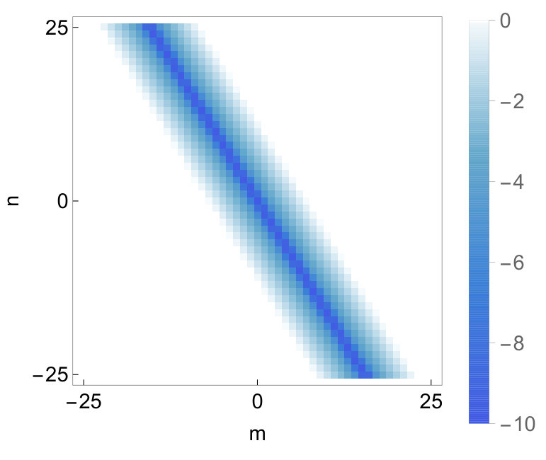 Figure 1
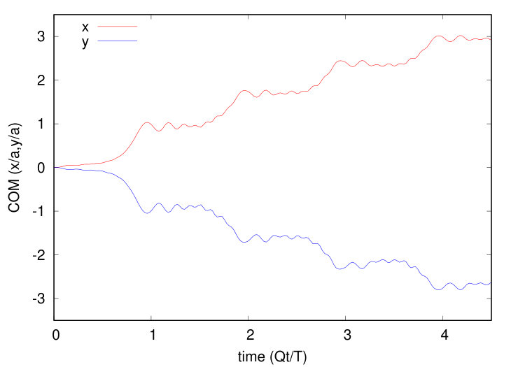 Figure 10
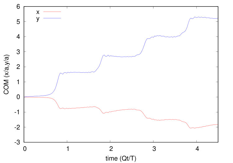 Figure 10
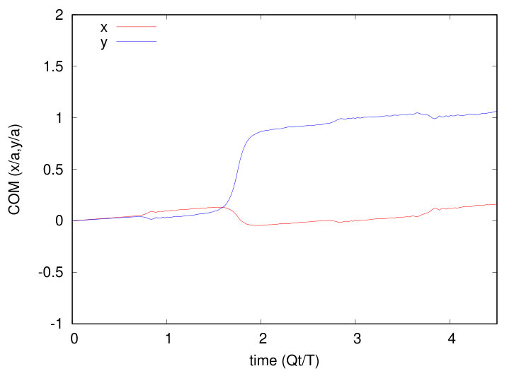 Figure 11
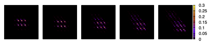 Figure 12
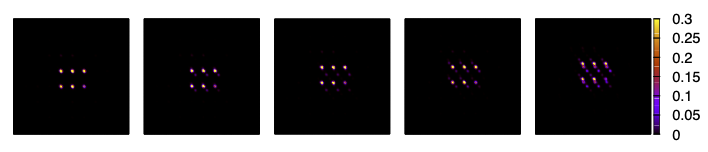 Figure 12
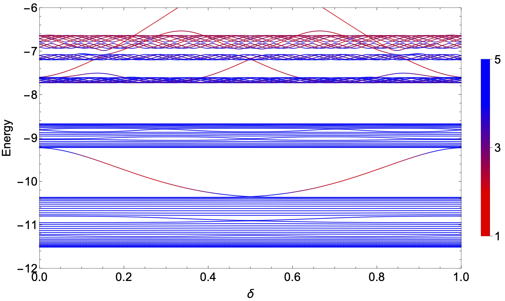 Figure 2
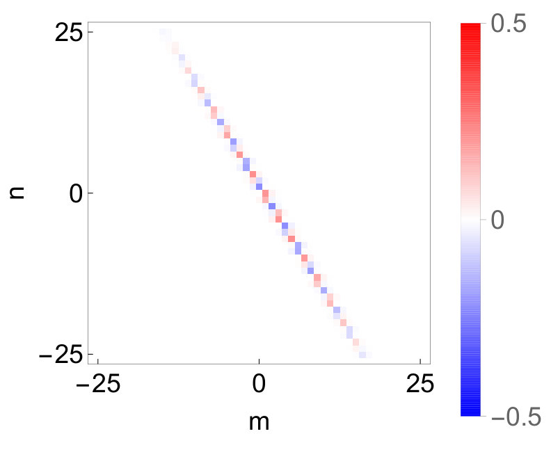 Figure 3
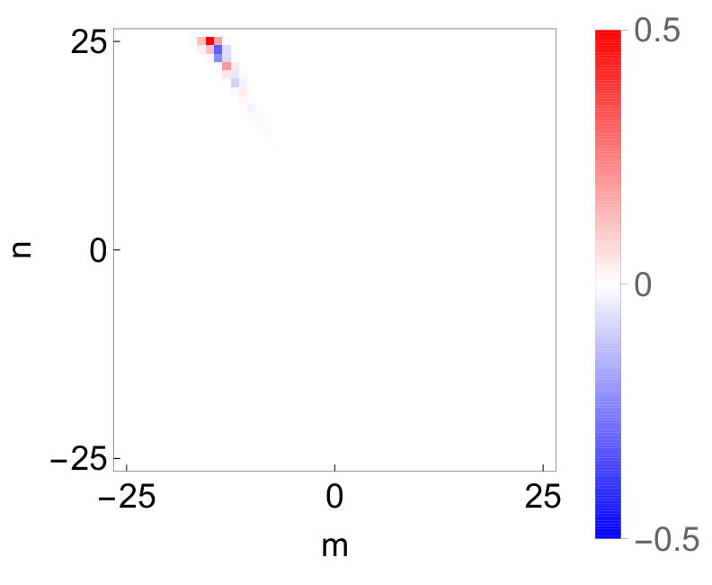 Figure 3
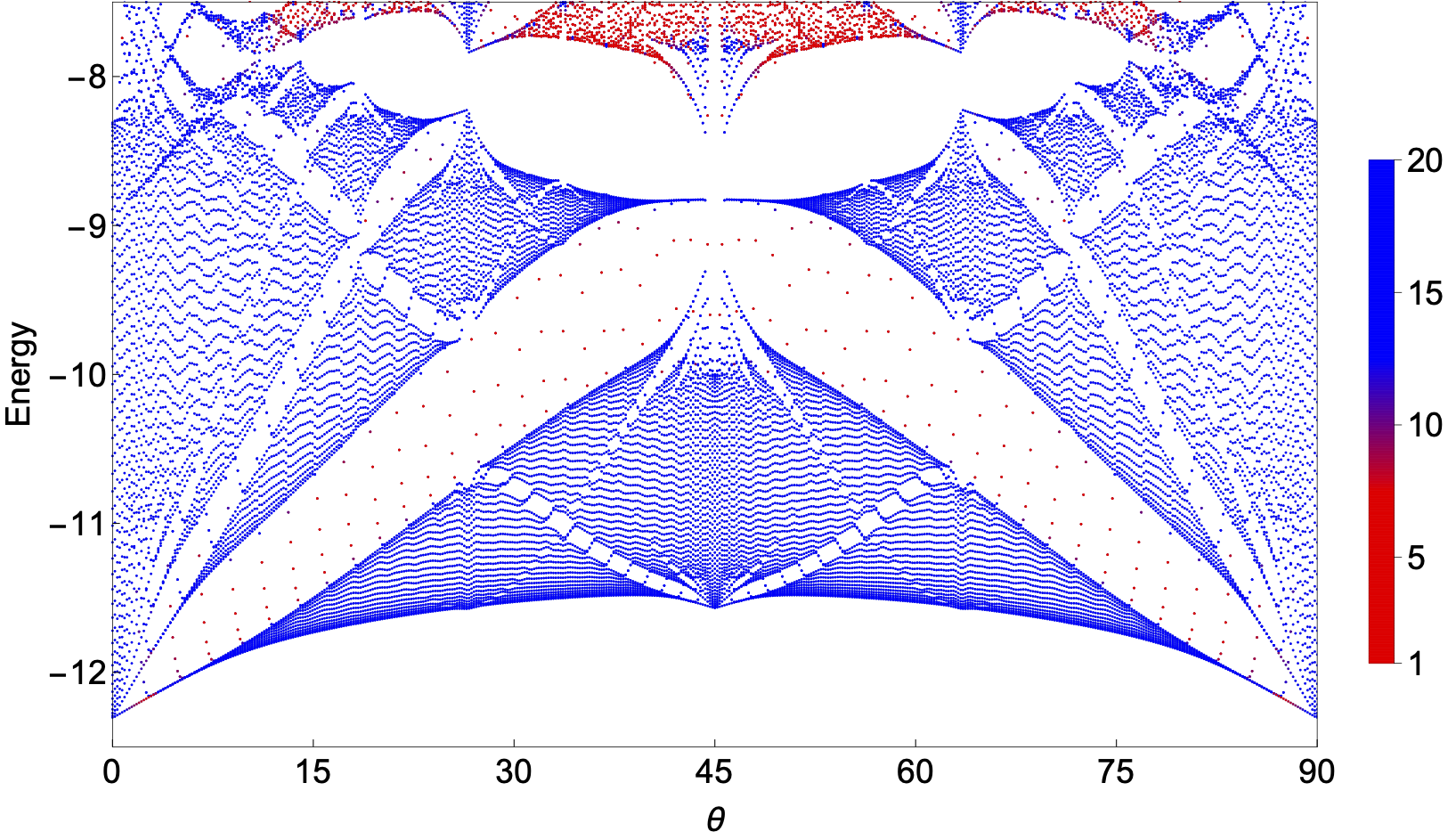 Figure 4
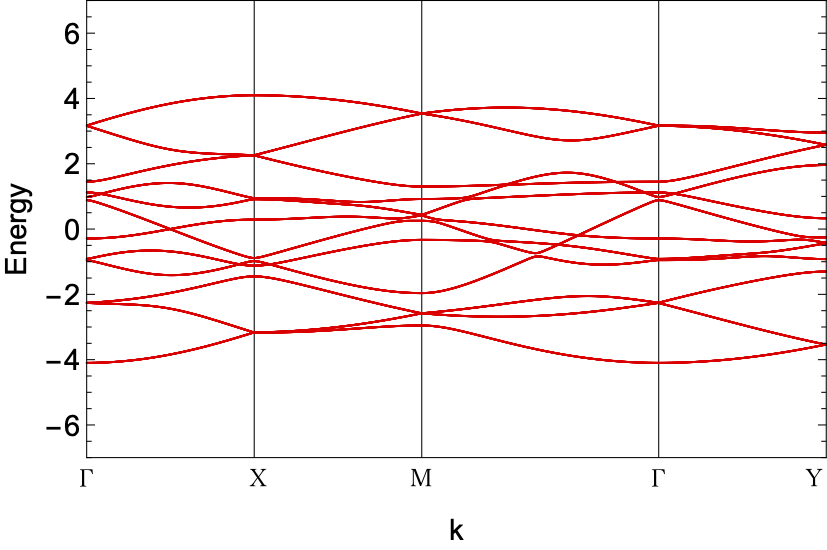 Figure 5
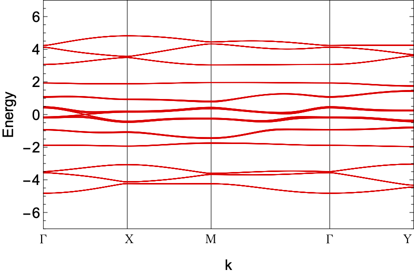 Figure 5
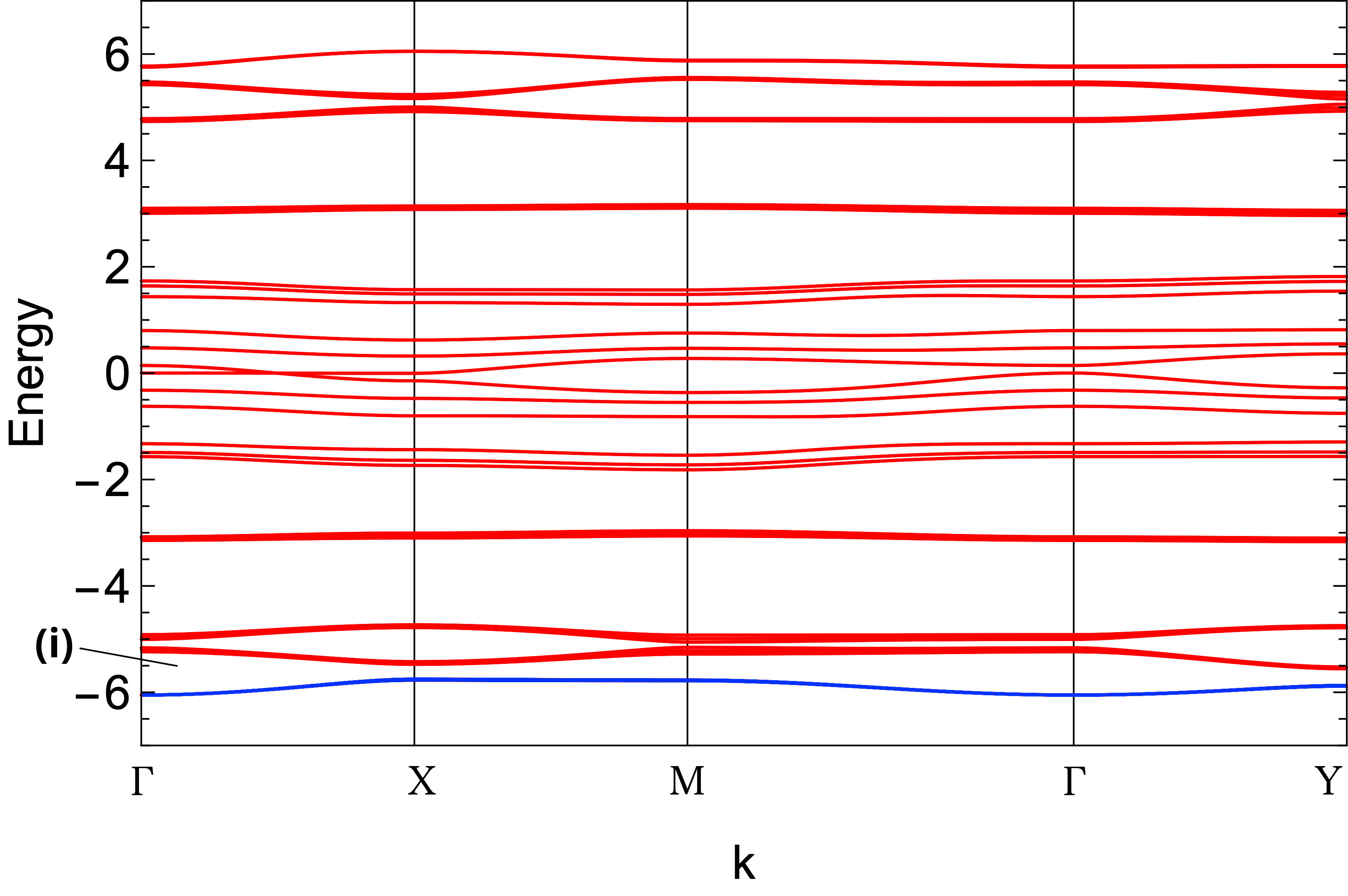 Figure 5
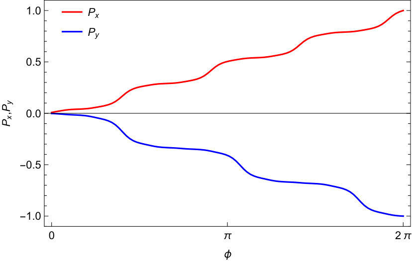 Figure 6
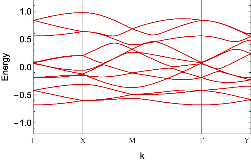 Figure 7
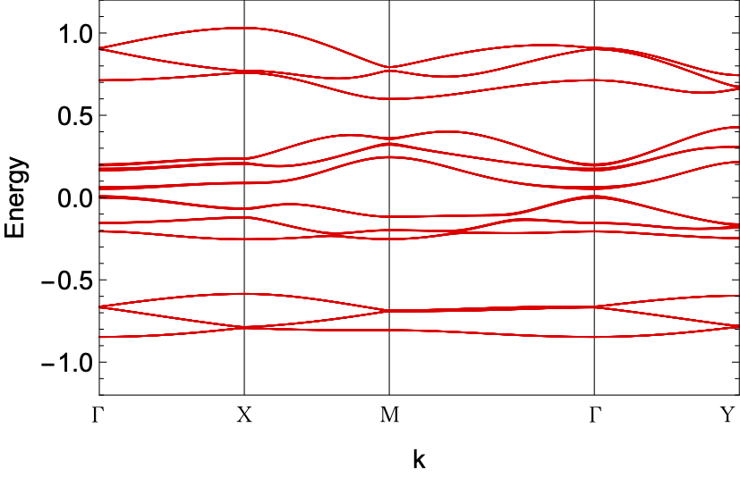 Figure 7
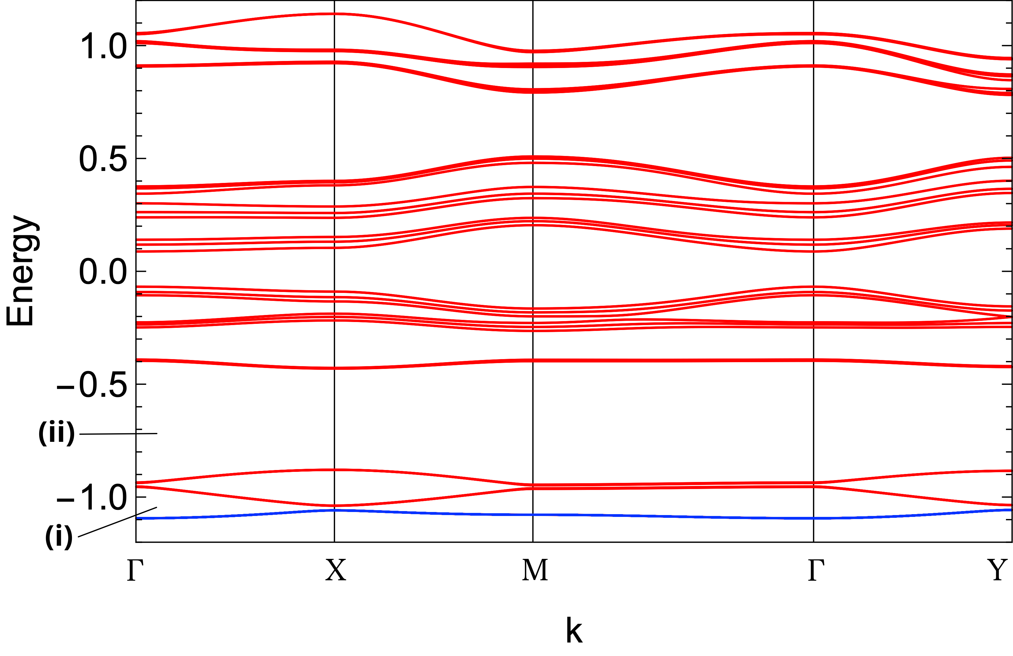 Figure 7
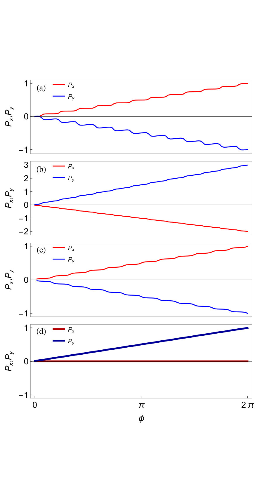 Figure 8
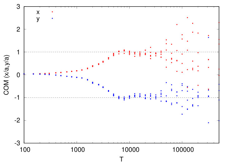 Figure 9
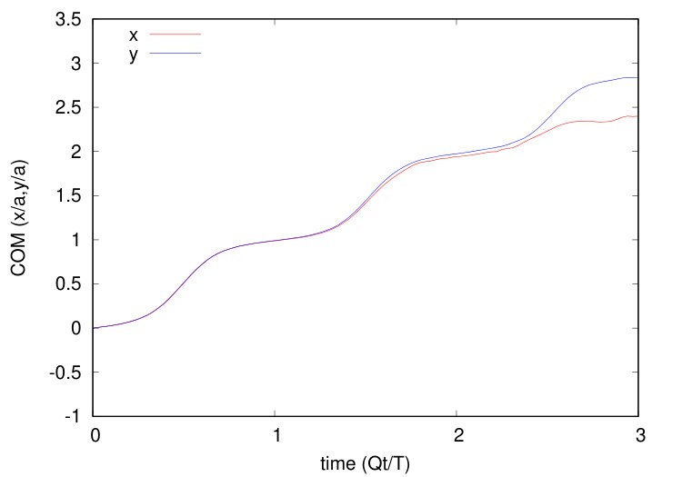 Figure 20
| 2 | 3 | 2 | 3 | 4 | 2 | 3 | 4 | 5 | 6 | |
| 3 | 4 | 5 | 5 | 5 | 7 | 7 | 7 | 7 | 7 | |
| 1 | 1 | 1 | -1 | 1 | 1 | 1 | -1 | -2 | 1 | |
| -1 | -1 | -2 | 2 | -1 | -3 | -2 | 2 | 3 | -1 |
| 0 | 1 | 2 | 3 | ||||
|---|---|---|---|---|---|---|---|
| 0 | 1 | -1 | 0 | ||||
| 0 | -1 | 2 | 1 |
Peer Reviews
No public reviews on file for this paper yet. If you reviewed it on a platform where reviews are public (OpenReview, ICLR, NeurIPS, ICML), you can paste yours below so the community can read it here.
Videos
No videos yet. Explain this paper in a talk, walkthrough, or lecture? Add one.
Two-Dimensional Thouless Pumping of Ultracold Fermions in Obliquely Introduced Optical Superlattice
Fuyuki Matsuda
Department of Physics, Kyoto University, Kyoto 606-8502, Japan
Masaki Tezuka
Department of Physics, Kyoto University, Kyoto 606-8502, Japan
Norio Kawakami
Department of Physics, Kyoto University, Kyoto 606-8502, Japan
Abstract
We propose a two-dimensional (2D) version of Thouless pumping that can be realized by using ultracold atoms in optical lattices. To be specific, we consider a 2D square lattice tight-binding model with an obliquely introduced superlattice. It is demonstrated that quantized particle transport occurs in this system, and that the transport is expressed as a solution of a Diophantine equation. This topological nature can be understood by mapping the Hamiltonian to a three-dimensional (3D) cubic lattice model with a homogeneous magnetic field. We also propose a continuum model with obliquely introduced superlattice and obtain the amount of pumping by calculating the Berry curvature. For this model, the same Diophantine equation can be derived from the plane-wave approximation. Furthermore, we investigate the effect of a harmonic trap by solving the time-dependent Schrödinger equation. Under a harmonic trap potential, as often used in cold atom experiments, we show, by numerical simulations, that nearly quantized pumping occurs when the phase of the superlattice potential is driven at a moderate speed. Also, we find that two regions appear, the Hofstadter region and the rectifying region, depending on the modulation amplitude of the superlattice potential. In the rectifying region with larger modulation amplitudes, we uncover that the pumping direction is restricted to exactly the -axis or the -axis direction. This difference in these two regions causes a crossover behavior, characterizing the effect of the harmonic trap.
pacs:
I Introduction
Intensive studies of the quantum Hall effect have opened up a wide research area known as topological phases RevModPhys.82.3045 ; RevModPhys.83.1057 . Topological phases are characterized by the associated invariants, which are prohibited from varying unless the energy gap closes. Moreover, topological phases have a characteristic property called the bulk-edge correspondencePhysRevB.23.5632 ; PhysRevB.25.2185 ; PhysRevLett.71.3697 ; RevModPhys.83.1057 , which guarantees the existence of the edge states, meaning that electrons can only move on the edge of a given material, as long as the bulk topological invariant has a nontrivial value. In quantum Hall systems, the topological invariant is defined by the Chern numberPhysRevLett.49.405 ; PhysRevLett.51.51 ; PhysRevB.31.3372 ; KOHMOTO1985343 , and it appears as the quantized Hall conductance. Similar relationships also appear in three-dimensional (3D) quantum Hall systemsPhysRevB.41.11417 ; PhysRevB.45.13488 ; Koshino2001 ; Koshino2002 .
Topological phases can be realized in various experimental platforms, not only in materials, but also in, for example, optical waveguidesKraus2012 and photonic systemsPhysRevA.84.043804 ; NaturePhys.7.907 ; NatureMat.12.233 . In particular, a great amount of effort has been made to realize topological insulators in cold atom systems by using synthetic gauge fields, which are induced by an optical latticeDalibard2011 . Various topological systems have been realized in cold atom systems, for instance, the Su–Schriefer–Heeger model Nature.9.795 , the Hofstadter model PhysRevLett.111.185301 ; PhysRevLett.111.185302 , synthetic dimensions Mancini1510 ; Stuhl1514 , and the Haldane model Nature.515.237 . Recently, topological charge pumping, called Thouless pumpingReview1983 ; PhysRevB.34.5093 , has been realized in cold atom systems NaturePhys.12.296 ; NaturePhys.12.350 , and many theoretical proposals have been made in numerous studiesPhysRevA.57.R2278 ; PhysRevA.76.052304 ; PhysRevA.84.013608 ; PhysRevLett.111.026802 ; PhysRevA.90.063638 ; PhysRevA.92.013612 ; PhysRevA.92.013609 ; Marra2017 ; PhysRevB.98.165128 ; JPSJ.83.083707 ; marra2020topologically ; PhysRevB.98.115147 ; PhysRevLett.118.230402 ; PhysRevA.95.063630 ; PhysRevB.98.245148 ; PhysRevLett.120.106601 ; PhysRevB.100.064302 ; PhysRevA.101.053630 ; Arceci_2020 . Also, two-dimensional (2D) Thouless pumping, where the nonlinear response is characterized by a four-dimensional (4D) topological invariant, is reported in Ref. Nature.553.55, .
Mapping the Hamiltonian between different dimensions plays an important role in understanding topological properties. One of the significant examples of mapping can be seen in the problem of the Hofstadter butterflyPhysRevB.14.2239 . Hofstadter mapped a 2D system of square lattice under a uniform magnetic field to a one-dimensional (1D) equation, which is called the Harper equation. Interestingly, in a recent study of Thouless pumping, this mapping was used backwards, and the topological equivalence over a certain group of Hamiltonians was shown. This kind of mapping to higher dimensions can be applied not only to 1D systems, but also to 2D and higher dimensional systemsKraus2013 .
In this study, we investigate topological properties for a 2D tight-binding model of particles that hop on a square lattice in the presence of modulation in the on-site potential, where the modulation amplitude depends only on the distance from an inclined line. We find that this model has a topological nature that can be understood clearly by applying a mapping from this 2D system to the corresponding 3D system. We show that the amount of pumping after the phase of the superlattice is adiabatically changed by one cycle is represented by a set of Chern numbers, which correspond to the solution of a Diophantine equation.
Furthermore, we consider a continuum model to confirm the result of the tight-binding model, and also to take the multiband effect fully into account. In the continuum model, as have been employed in Ref. Wang2013, , the contribution of the higher bands is included, while it is ignored in the tight-binding model. We discuss Thouless pumping by using the plane-wave approximation as a counterpart of the tight-binding model. Moreover, we investigate how the harmonic trap affects our model by solving the time-dependent Schrödinger equation. We show that nearly quantized pumping occurs when the phase of the superimposed potential is changed at an appropriate speed. We find that the pumping behavior is different between two regions: In the Hofstadter region with smaller modulation amplitudes, the amount of pumping obeys the Diophantine equation, while in the rectifying region with larger modulation amplitudes, the pumping direction is restricted to exactly the -axis or the -axis direction. This difference causes a crossover behavior, highlighting the effect of the harmonic trap.
This paper is organized as follows. In sect. 2, we introduce a 2D square lattice tight-binding model with an obliquely introduced potential in order to investigate the effect of the superimposed potential in the context of topological phases. In sect. 3, we study a continuum model that corresponds to the above-mentioned tight-binding model. In sect. 4, we conclude our paper.
II Topological Aspects of 2D Optical Lattice with Obliquely Introduced Potential
II.1 Model
Recently, the development of experimental techniques regarding cold atoms in an optical lattice has been remarkablePhysRevA.69.013603 ; RevModPhys.80.885 , and the degree of freedom in designing a quantum simulation is high. TriangularBecker_2010 , squareYang , and hexagonal latticesnphys1916 have all been realized in cold atom systems. Moreover, it is possible to realize nonstandard lattices in cold atom systems. One example of such lattices is the lattice made by superimposing a typical lattice potential and a superlattice potential. For example, in Ref. Taiee1500854, , Taie et al. realized an optical Lieb lattice by adding a diagonal lattice to a conventional square optical lattice. By taking advantage of these high degrees of freedom of the optical lattice, various topological phases have been proposed theoreticallyPhysRevLett.100.070402 ; PhysRevA.79.053639 ; PhysRevB.84.165115 ; PhysRevA.86.031603 ; PhysRevA.82.013608 ; PhysRevA.93.043617 ; PhysRevA.94.043611 ; PhysRevA.96.032103 ; PhysRevLett.121.133002 and realized experimentallyGoldman6736 ; ncomms2523 ; doi:10.1063/1.5087957 ; NatPhys.15.911 ; deLeseleuc775 ; RevModPhys.91.015005 . In particular, the cold atom system is one of the most suitable platforms for realizing Thouless pumping. Various types of Thouless pumping have been realized in cold atom experimentsNaturePhys.12.296 ; NaturePhys.12.350 ; PhysRevLett.117.170405 ; Nature.553.55 .
Also, this study is partly motivated by recent remarkable progress in solid-state physics, i.e. twisted bilayer graphene (TBG). TBG has been receiving much attention lately because of the realization of unconventional superconductivityNature26160 . TBG has been investigated in many contexts, such as its electronic structuresPhysRevLett.99.256802 ; ROZHKOV20161 , flat bandsPhysRevB.82.121407 , topological band structuresPhysRevB.84.045436 , and Moiré butterfliesPhysRevB.84.035440 . It also provides a prototypical example of superimposed lattice potential.
Stimulated by the above-mentioned previous studies, it is natural to ask what happens if the additional diagonal lattice in the optical Lieb lattice is angled. Here, as a paradigmatic example, we consider a Fermi gas loaded in a 2D optical square lattice with a superlattice structure that is introduced obliquely. The lattice constant is taken to be unity. We study the topological properties of the system, which is described by the following Hamiltonian:
[TABLE]
where is the fermion creation (annihilation) operator, is the hopping strength, is the parameter of the real-space potential shift, is the normal vector of the superlattice direction, and is the distance from the line expressed by . The boundary conditions are taken as either open or periodic. Below, we take as the unit of energy.
II.2 Obliquely Introduced Single Well
First, we consider the case that has a single dip, where the Hamiltonian has an oblique linear single well. We take , as the linear-shaped potential, which restricts particles from moving around the potential in the low-energy region. The on-site potential in this system is plotted in Fig. 1. As a consequence of the overlap of the square lattice and the obliquely introduced potential, this model can be effectively considered as a 1D tight-binding model with a superlattice. This effective superlattice opens the energy gap. By analogy to the previous studies of topological aspects of a 1D superlatticePhysRevLett.108.220401 ; Kraus2012 ; JPSJ.83.083707 , the edge states will appear when we drive the phase of the superlattice, which corresponds to the parameter in this model. In Fig. 2, we diagonalize the tight-binding model, which is described in Eq. (1), with the system size and under open boundary conditions. Figure 2 shows the plots for the bottom part of the energy spectrum since the upper part of the spectrum has no band gap because of the 2D nature of the wave function. We can see the existence of band-crossing states in the energy spectrum with open boundary conditions as a function of in Fig. 2. The color in the figure shows the participation ratio (PR), which is defined as
[TABLE]
A small PR indicates that the eigenfunction is well localized. Note that the bulk band is fixed because we choose an irrational number for tangent . Figures 3(a) and 3(b) respectively show the wave functions of an in-band state and a band-crossing state. We confirm that the wave function of the band-crossing state is localized around the edge.
With changing , the distribution of the energy band also changes. Figure 4 shows the energy spectrum plotted against tilting angle , which is related to through the formula . We diagonalize the tight-binding model with the system size and under open boundary conditions. For the same reason as in Fig. 2, Fig. 4 shows the plots only for the bottom part of the energy spectrum. As shown in the figure, a butterfly-like structure appears in the energy spectrum plot. This structure is similar to the “3D butterfly” introduced in Refs. Koshino2001, and Koshino2002, . We will explain the origin of this similarity later. The color in Fig. 4 represents the PR in each eigenfunction, which is defined in Eq. (6). We can see that the eigenstates in the band gap are well localized, corresponding to edge states in topological systems.
The upper part of Fig. 4 also shows many localized states, but this is not the point we want to focus on because the wave functions in this region are no longer quasi-1D.
II.3 Obliquely Introduced Superlattice
As we have seen in the previous section, the band-crossing states and the edge-localized states appear when is a single well, exemplifying the topological nature of the effective 1D system. We will now discuss topological properties in two dimensions when is a periodic function. As a typical periodic function, we take . In this case, when we vary slowly, the Hamiltonian will be periodic in time, and this setup corresponds to the adiabatic transport, first proposed by ThoulessReview1983 .
It is known that a mapping between a 1D superlattice system and a 2D Hofstadter model existsKraus2012a . Analogously, we can clearly understand the topological aspects of our model by mapping it to a 3D Hamiltonian. For simplicity, we start our discussion with the case that is a rational number. The Hamiltonian can be rewritten as follows:
[TABLE]
where and determine the periods for the - and -directions of the Hamiltonian, respectively. Also, we use as a parameter controlling the phase of the cosine-type potential. We can map this Hamiltonian to a 3D Hamiltonian by using the Fourier transformation,
[TABLE]
Hamiltonian (7) will become
[TABLE]
This Hamiltonian describes a 3D tight-binding model on the cubic lattice with a homogeneous magnetic field whose direction is perpendicular to the -axis but oblique in the -plane. This model has been previously studied, and it is known that the Hofstadter butterfly and the integer quantum Hall effect (IQHE) also appear in the 3D latticePhysRevB.41.11417 ; PhysRevB.45.13488 ; Koshino2001 ; Koshino2002 . According to Refs. Koshino2001, and Koshino2002, , each gap in the 3D Hofstadter butterfly is characterized by two Chern indices. In the 3D model, these indices are proportional to the Hall conductivity. When we go back to our 2D model, these indices determine the topological pumping, just like Thouless pumping, and the bulk-edge correspondence shows that the amount of pumping and the number of edge states match each other. In this model, the amount of pumping in the - and -directions corresponds to the number of localized states at edges of - and -directions, respectively. Also, by comparing (7) and (10), we can see that potential strength corresponds to the hopping strength in the -direction. These correspondences explain why the 3D butterfly appears in Fig. 4.
Here, we have only considered a cosine-type potential, but a similar mapping is also possible for other types of potentials for which there are higher frequency components, and these components will be mapped to longer distance hoppings in the -direction.
II.4 Diophantine Equation
By mapping the Hamiltonian, we have seen that the Chern number characterizes the system, but how does the Chern number appear in observables? This question can be solved by considering the polarization. Since the derivative of the polarization is proportional to the current, the amount of pumping is proportional to the total amount of change in the polarization. Now, let us briefly summarize the theory of polarization.
According to Ref. Resta2007, , the polarization has an integer ambiguity by a multiple of the lattice constant, but the change of the polarization in the course of a continuous change in the Hamiltonian can be defined without ambiguity. When we write the wave vector of the electronic wave function as , the change in the polarization can be written as
[TABLE]
[TABLE]
where is the parameter of the Hamiltonian, is the area of the Brillouin zone, and the charge of an electron is . The expression for the integrand has the same form as the Berry curvaturedoi:10.1098/rspa.1984.0023 .
Following the above formula for the change in the polarization, we can define the amount of pumping even in infinite systems. Namely an analogy with Eqs. (11) and (12) enables us to express the amount of pumping in the - and -directions for our 2D system when is increased from to as
[TABLE]
[TABLE]
In the presence of the superlattice potential, the lattice periodicity is multiplied by and for the - and -directions, respectively. Therefore, the size of the first Brillouin zone shrinks by . This can be regarded as an analog of the magnetic Brillouin zoneinverse . We note that the signs in Eqs. (13) and (14) are opposite to the counterpart in Eq. (12) because of the sign of an electron charge.
Considering the case where is periodic with period , the amounts of pumping in - and -directions in one period for our 2D system are written as
[TABLE]
[TABLE]
The formula in the square brackets in Eqs. (15) and (16) has the same form as the definition of the Chern number on the torus created by and , respectively. The Chern number is guaranteed to be an integer, but is not necessarily an integer because it is given by the average of Chern numbers. However, if changing does not close the band gap, then neither does the Chern number change, so is also an integer. To summarize, in an adiabatic time-periodic system, the amount pumped in the -direction during one period is represented by the integral of the change in polarization in the -direction, which corresponds to the average in the -direction of the Chern numbers for .
As we have mentioned above, in the tight-binding approximation, we can map our model to a 3D cubic lattice model with an obliquely introduced homogeneous magnetic field in Eq. (10), and the amount of Thouless pumping in our model corresponds to the quantized Hall conductance in the cubic lattice model. In Eq. (10), and are cyclic coordinates, so that the wave function can be written as , where and are the Bloch wave numbers along the - and -directions, respectively. Then the Schrödinger equation will be
[TABLE]
This equation is equivalent to a 3D version of the Harper equation. By analyzing this equation, the following Diophantine equation can be obtained PhysRevB.45.13488 :
[TABLE]
Here, is the number of filled bands and is the least common multiple of and . and correspond to the amounts of pumping when changes from [math] to . The detailed derivation of this equation is shown in Appendix A.
Below we focus on the case where and are coprime. Then Eq. (18) can be transformed to
[TABLE]
Basically, we are concerned with the lowest band, so we should consider the case . Table 1 shows the solution of Eq. (19) in several cases.
II.5 Band Structure and Pumped Amount
In the previous section, we showed that the amount of pumping obeys a Diophantine equation. Now we show a concrete example below. In particular, we focus on the case where .
Figure LABEL:TBband shows how the band changes when the magnitude of the modulation of the onsite potential is changed. Figures LABEL:TBband(a)–(c) are the band structures for , respectively. When is large, the lowest band gap (i) is opened, which can be observed in Fig. LABEL:TBband(c). On the contrary, when is small, the Berry curvature cannot be calculated well since the band gap is small. The smaller the band gap, the larger the number of meshes required for the Fukui–Hatsugai–Suzuki method. The reason why the band gap is so small is that the higher order perturbations open the gap. It is not likely that the band gap is closed in the process of increasing , so it seems that the gap is open even if is very small, but is too small to be detected numerically.
Here we investigate the amount of pumping for the lowest band in Fig. LABEL:TBband(c). We apply the Fukui–Hatsugai–Suzuki methoddoi:10.1143/JPSJ.74.1674 to calculate the amount of pumping, which can be obtained by integrating the Berry curvaturedoi:10.1098/rspa.1984.0023 . The specific expression for the amount of pumping is given in Eqs. (13) and (14). Figure 6 shows the amount of pumping for large , which is calculated using Eqs. (13) and (14). The amount of pumping after one cycle, and , agrees with the solution of the Diophantine equation shown in Table 1.
III Continuum Model of 2D Thouless Pumping
III.1 Model
In light of the analogy of Thouless pumping and the IQHE, the results in the previous section suggest that the amount of transport, as the Hamiltonian parameter changes its value from 0 to , is quantized and can be expressed in terms of the Chern number. Since the discussion in the previous section is based on the tight-binding model, it is desirable to extend our discussion to continuum systems so as to apply the results to cold atom systems. To treat the system more precisely and to see the feasibility of the previous model in the experimental setups, we next consider a 2D continuum model.
To be specific, we consider the following Hamiltonian:
[TABLE]
where is the field operator of a particle, is Planck’s constant, and is the mass of a particle. There are three types of potentials in this system: , , and . and form the 2D square lattice, and forms the superlattice oblique to the square lattice. Henceforth, we take as the unit of energy.
III.2 Plane-Wave Approximation
III.2.1 Band Structure
We now apply the plane-wave approximation to the Hamiltonian introduced in Eqs. (22)–(22) to calculate the eigenenergies and the wave functions directly. First, we apply the Fourier transformation
[TABLE]
to Eq. (22). Then, we obtain the following Hamiltonian:
[TABLE]
When the condition is satisfied, it is possible to diagonalize Eq. (24) numerically by introducing the cutoff for wavenumbers and .
Figure LABEL:PWband shows the band structure when the plane-wave approximation is used. In order to calculate the wave function under the plane-wave approximation, we introduce the cutoff of wavenumber . To be specific, we only consider small and satisfying the condition in Eq. (24). The band structure is similar to that in Fig. LABEL:TBband when is small, but the gap begins to increase as increases, and the first gap is clearly open in the plot for . Even in this model, it is unlikely that a phase transition accompanied by gap formation occurs somewhere, so we expect that a gap opens even if is small. When is small, the gap is formed by a higher order perturbation, which is probably not visible in the figure.
III.2.2 Pumped Amount and Diophantine Equation
Figure 8(a) shows the amount of pumping for the ground state under the condition . Since we use the plane-wave approximation to calculate wave functions, there are an infinite number of bands. Only the low-lying bands are plotted. In this case, a single band corresponds to the filling. The amount of pumping after one cycle is -1 in the -direction and +1 in the -direction, which is consistent with the solution of the Diophantine equation. Also, the pumping proceeds stepwise in 12 steps. This is consistent with . In general, we suppose that the amount of pumping calculated in the plane-wave approximation follows the same Diophantine equation as in the tight-binding limit. The justification of the equation is given in Appendix B.
We here focus on the fact that the band gap between the second and third excited states is large in Fig. LABEL:PWband, requiring us to treat the low-lying states below the gap carefully. Figures 8(b) and 8(c) show the amount of pumping of the first excited state and the second excited state, respectively. Also, Fig. 8(d) shows the total amount of pumping of the states in Figs. 8(a)–8(c). As mentioned earlier, the amount of pumping is also represented by the Diophantine equation (18) within the plane-wave approximation. Concretely, the amount of pumping when the corresponding state is located from the bottom to the th state is the solution of Eq. (18). Therefore, if we denote the th pair of Chern numbers from the bottom as and the solution of Eq. (18) for as , we have , . Table 2 shows the solutions of Eq. (19) for of Eq. (18) and the difference between them for . The amount of pumping after one period () corresponds to the differences between the adjacent solutions of the Diophantine equation, , , and , which are listed in Table 2. These are consistent with Fig. 8. Also, Fig. 8(d) corresponds to the solution for in Table 2.
We suppose that the wide band gap in is generated by a first-order perturbation, while other gaps are generated by higher order perturbations. The bold lines in Fig. 8(d) show the amount of pumping when the states are filled up to this wide band gap. In the present case, instead of dealing only with the lowest band, we sum up the contributions of the three bands from the bottom, as already mentioned. Then, the pumping in the -direction becomes zero, and only the pumping in the -direction remains.
We also compute the Chern numbers for various cases with different and . These include the case of , where both and have absolute values of 2 or larger. In every case, and obey the Diophantine equation (18). These results validate the claim that a pair of Chern numbers are determined by the Diophantine equation from the calculation of the Berry curvature.
III.3 Effects of Harmonic Trap
So far, we have studied the continuum model (22) in the infinite system having -site periodicity with an integer number of filled bands. We have seen that the amount of pumping is quantized and the Chern numbers obey the Diophantine equation in the infinite system. In this section, we discuss the effect of a harmonic trap on the continuum model. We consider the following Hamiltonian, where the harmonic potential is added as a trap to the continuum model Hamiltonian (22), and simulate the time evolution of the lowest-energy states and their center of mass (COM).
[TABLE]
For the initial state, we employ the eigenstates calculated for the initial superlattice potential. We set when one of the lattice minima is on the minimal line of the superlattice potential. Starting from , we solve the time-dependent Schrödinger equation using the infinitesimal time evolution operator while the superlattice potential is changing. We set the mesh size to and the time step to .
When the harmonic potential exists, the difference in the COM of the wave functions of the occupied states corresponds to the amount of pumping. Let be the initial COM at . These are not necessarily 0. We will plot the change in the COM, which is expressed as , . Below, we take the average COM of the five lowest energy states. Even if we change the number of states, the change in the COM does not significantly affect the amount of pumping owing to the harmonic potential, but in this case, we set the number of states to five to avoid edge effects. We can discuss the pumping behavior in terms of the computed COM.
In the presence of a harmonic trap, the pumping behavior turns out to be completely different between two regions. One is the weak superlattice region, in which is small compared with (which is called the Hofstadter region), and the other is the strong superlattice region, in which is large (which is called the rectifying region).
III.3.1 Hofstadter Region
First, we consider the region near the tight-binding limit, i.e. , where denotes the recoil energy RevModPhys.80.885 . In the previous discussions, we calculated the amount of pumping by considering the integral of the Berry curvature, but this corresponds to the amount of pumping when the perfectly adiabatic process is achieved. In the present case with a trap potential, we must solve the time-dependent Schrödinger equation represented by Eq. (25). We need a new parameter of one cycle time . In practice, the perfectly adiabatic process cannot be realized. Although the quantization of the amount of pumping is lost due to the effect of the harmonic trap and the loss of the adiabaticity, the correct tendency remains for the direction and the amount of pumping.
Figure 9 shows the COM for the five states with the lowest energy for various time periods . It shows that when is chosen so that the pumping is performed at appropriate speeds, the COM after one cycle is around . We can see that plateaus are found in the middle of the figure. In other words, the solutions to the Diophantine equation, discussed in the previous section, appear as the amount of pumping only when is in the range of intermediate speeds. Here, we discuss why the plateaus appear in Fig. 9. There are three important time scales, the period of the cycle , the inverse of the band-gap size , and the inverse of the depth of the harmonic trap . When is much smaller than , the pumping procedure is too fast and cannot be regarded as an adiabatic process. On the other hand, when is much larger than , there is enough time for the COM of particles to return to the initial position, that is, the center of the harmonic trap. As a result, should be between and to observe clear pumping behavior. In other words, if is too small, the particles will not be able to follow the motion of the superlattice and will be left behind, while if is too large, because of the harmonic trap effect, the pumping does not work properly.
Figure 10 shows concrete examples of such pumping. Figures 10(a) and 10(b) show the time evolutions of the COM for the five lowest-energy states in the case of and , respectively. According to Fig. 10, particles are pumped in the direction for (a) and the direction for (b). Surprisingly, while the direction of the superlattice is changed only slightly, the pumping direction is completely changed. This pumping direction can be predicted by solving Eq. (18) with the condition since the contribution of the lowest band is dominant. For example, in case (a), the solutions of Eq. (18) are with integers and . and correspond to the order of perturbation. Therefore, although there are an infinite number of solutions, only the solution where and have the smallest values is dominant. In case (a), this solution is . Similarly, in case (b), the solution of the Diophantine equation is , and the dominant solution is . These results are consistent with Fig. 10.
Observing Fig. 10 carefully, we find a small oscillation after the particle was pumped to the next lattice minimum. This oscillation occurs at the moment when the ground-state energies at two sites become close. At that moment, the potential shape can be approximated by a double well, and the particles oscillate between the two wells. Since the angular frequency of this oscillation will be the same as the hopping amplitude , the period will be . To estimate in the optical lattice, we can use , where . We have checked that this estimate is consistent with the numerical result in Fig. 10. We have also verified that the frequency of this small oscillation does not change when we change the time period . This result implies that the small oscillation is caused by the pumping, which is performed in a finite time.
Throughout this paper, we have focused on the case of , but the Diophantine equation (18) can also be applied to other cases. For the case where and , see Appendix C.
III.3.2 Rectifying Region
In the opposite region, where the term is dominant, the pumping behavior changes completely. From our numerical simulation, we find that the pumping direction is restricted to the exactly -axis or the -axis in this region. More precisely, the pumping direction will be the -axis or the -axis, whichever is closer.
When varies across the Hofstadter region to the rectifying region, a crossover occurs. Figures 10(a), 11, and 12 provide concrete examples of such a crossover. Figures 10(a) and 11 show the time evolution of the COM for the five lowest energy states in the case of , with (a) and (b) . We note that only the difference in the superlattice potential depth causes the change in pumping direction. Figures 12(a) and 12(b) show the time dependence of particle density profiles computed under the conditions corresponding to Fig. 10(a) and Fig. 11, respectively. We can clearly see that particles move in different directions depending on whether is small or large.
The band structure in the previous section gives us a hint to understand why this crossover happens. The solution of the Diophantine equation with appears when only the lowest band is considered, and pumping occurs in both the - and -directions. On the contrary, if we compute a state that is lower than the wide band gap, pumping will occur only in the - or -direction. The result in Fig. 11 suggests that the state below this wide band gap is occupied in this region. A system containing a harmonic trap has the property that a wide band gap is automatically selected without adjusting the number of particles. In the present case, by changing , the width of the band gap also changes, and the crossover will be caused by the change in the band gap, which is automatically selected by the effect of the harmonic trap.
We note that such a change in the direction of pumping has also been studied by Lohse et al.NaturePhys.12.350 . In Ref. NaturePhys.12.350, , the topological transition in 1D systems is reported, where the Chern number of excited states is changed. On the other hand, the crossover found in our study is due to the effect of the harmonic trap. Since the coefficients in the Bloch wave expansions of the trapped eigenstates evolve continuously as functions of and are not quantized because of the effect of the harmonic trap, quantization of the pumping is incomplete and the topological transition does not occur.
IV Conclusion
We have proposed a 2D version of Thouless pumping by employing a 2D square lattice tight-binding model with an obliquely introduced superlattice. We have shown that quantized particle transport occurs in this system, and the transport is expressed as a solution of a Diophantine equation. This topological nature can be understood by mapping the Hamiltonian to a 3D cubic lattice model with a homogeneous magnetic field. Moreover, we have investigated how the harmonic trap affects our model by solving the time-dependent Schrödinger equation. We have shown that plateaus appear in the plot of the COM against the time period for superlattice sliding. When is in the plateau region, nearly quantized pumping is achieved. We have found that the pumping behavior is different in two regions, which we call the Hofstadter region and the rectifying region. In the Hofstadter region, the amount of pumping obeys the Diophantine equation. On the contrary, in the rectifying region, the pumping direction is restricted to exactly the -axis or the -axis direction. This difference causes the crossover behavior, highlighting the effect of the harmonic trap.
In summary, we have shown that the amount of pumping in a 2D lattice with an obliquely introduced superlattice obeys a Diophantine equation, and the harmonic trap affects the pumping behavior in various ways. The effects of the interaction and the lattice deformation are left for future studies.
Acknowledgements.
This work was supported by JSPS KAKENHI (Grant No. JP18H01140, JP19H01838 (N. K.), Grant No. JP17K17822 and JP20H05270 (M. T.)) and a Grant-in-Aid for Scientific Research on Innovative Areas “Topological Materials Science” (Grant No. JP15H05855).
Appendix A Derivation of Diophantine Equation in Tight-Binding Limit
In this Appendix, we derive Eq. (18) from the Hamiltonian
[TABLE]
This Hamiltonian is periodic in with period . Here, we suppose that and are rational numbers, such as , where and are pairs of coprime integers with .
The Fourier-transformed Hamiltonian obtained by using Eq. (10) is
[TABLE]
Here, we have defined for convenience. However, there is mixing between and , and thus the Hamiltonian is not diagonal in . To diagonalize it, we must separate into regions as follows:
[TABLE]
Then, the Hamiltonian can be written as
[TABLE]
[TABLE]
Note that the Brillouin zone is reduced to for and for . Now, the Schrödinger equation is reduced to that for a 1D tight-binding model. The single-particle energy is obtained by expanding the state into single-particle states at each lattice point ,
[TABLE]
where is the vacuum. The eigenvalue equation is
[TABLE]
This corresponds to the Harper equation for the Hofstadter model. Let be the least common multiple of and , and let and be integers that satisfy , . For convenience, we perform the transformation
[TABLE]
and we obtain
[TABLE]
To solve this equation, we apply the perturbation theory under the condition . The solution at is
[TABLE]
If we make finite, gaps open at the degeneracy points. To understand this in detail, we should make the condition for degeneracy clear. When the two bands and cross each other, the degeneracy condition is
[TABLE]
The degeneracy only occurs when , so we can rewrite it as
[TABLE]
It is obvious that the lowest band corresponds to . It is possible to determine all of the band indices by using Eq. (40). There is a simple relation between the gap number and band indices :
[TABLE]
Now we are ready to use the perturbation theory. Since the term only mixes two sites that are sites apart from each other, in order to hybridize and , the following equation must be satisfied:
[TABLE]
that is,
[TABLE]
The lowest order of perturbation that mixes and is the th order for the term and the th order for the term, respectively.
The Hamiltonian around the th gap is
[TABLE]
Now, it is possible to calculate the amount of pumping in one cycle from this Hamiltonian. The amount of pumping will be for the -direction and for the -direction, and this is exactly the solution of the Diophantine equation (43). However, we should be aware that “one cycle” here corresponds to the width of the Brilliouin zone of , while changes its value by .
Appendix B Justification of Diophantine Equation in Plane-wave Approximation
In this Appendix, we derive Eq. (18) from the Hamiltonian given in Eq. (22). For simplicity, let . To make the perturbation theory easier to apply, we divide the Hamiltonian in Eq. (22) into and ,
[TABLE]
First, eigenstates of can be written in Bloch states in a Brillouin zone of size . If is added here, some Bloch states are hybridized. This is an idea just like the magnetic Brillouin zone. Let the Bloch state obtained from be and the corresponding eigenenergies be . The expression corresponding to Eq. (29) in Appendix A is
[TABLE]
This is not diagonal because it is mixed for different . However, we can diagonalize it by using a similar method to that in Appendix A. By expressing the single-particle states as a linear combination of different wave number states,
[TABLE]
then the eigenvalue equation is obtained as follows:
[TABLE]
Since the eigenenergies of the Bloch state do not change so much from the cosine function, the position of the degenerate point does not change. As a result, the degree of perturbation required is determined from the degenerate point condition, which leads to the same Diophantine equation.
Appendix C Pumping in the Case
Throughout this paper, we have focused on the case. However, the obtained Diophantine equation (18) is appliacable to other cases. In this Appendix, we show a concrete example for these cases.
Figure 13 shows the time evolution of the average COM in the case of where the harmonic potential exists. Since , is the solution of the Diophantine equation that corresponds to the lowest order of the perturbation. If we look at Fig. 13, we see that particles are pumped in the direction of the line . We can confirm that the pumping direction and the solution of the Diophantine equation also match each other in this case.
The reference list from the paper itself. Each links out to its DOI / PubMed record.
- 1(1) M. Z. Hasan and C. L. Kane, Rev. Mod. Phys. 82 3045 (2010).
- 2(2) X.-L. Qi and S.-C. Zhang, Rev. Mod. Phys. 83 1057 (2011).
- 3(3) R. B. Laughlin, Phys. Rev. B 23 5632 (1981).
- 4(4) B. I. Halperin, Phys. Rev. B 25 2185 (1982).
- 5(5) Y. Hatsugai, Phys. Rev. Lett. 71 3697 (1993).
- 6(6) D. J. Thouless, M. Kohmoto, M. P. Nightingale, and M. den Nijs, Phys. Rev. Lett. 49 405 (1982).
- 7(7) J. E. Avron, R. Seiler, and B. Simon, Phys. Rev. Lett. 51 51 (1983).
- 8(8) Q. Niu, D. J. Thouless, and Y.-S. Wu, Phys. Rev. B 31 3372 (1985).