Magnetic Levitation and Compression of Compact Tori
Carl Dunlea, Stephen Howard, Wade Zawalski, Kelly Epp, Alex Mossman,, General Fusion Team, Chijin Xiao, Akira Hirose

TL;DR
This paper reports on magnetic levitation and compression of compact toroids in a fusion experiment, demonstrating improved plasma stability, reduced impurities, and enhanced magnetic and thermal properties through optimized coil configurations and MHD modeling.
Contribution
It introduces an optimized coil configuration for better CT levitation and compression, and develops an energy-conserving MHD simulation to analyze plasma behavior.
Findings
Improved levitation field profile reduces plasma impurities.
Enhanced magnetic field, density, and ion temperature during compression.
Reduced MHD activity with matched coil decay rates improves CT longevity.
Abstract
The magnetic compression experiment at General Fusion was a repetitive non-destructive test to study plasma physics to Magnetic Target Fusion compression. A compact torus (CT) is formed with a co-axial gun into a containment region with an hour-glass shaped inner flux conserver, and an insulating outer wall. External coil currents keep the CT off the outer wall (radial levitation) and then rapidly compress it inwards. The optimal external coil configuration greatly improved both the levitated CT lifetime and the rate of shots with good flux conservation during compression. As confirmed by spectrometer data, the improved levitation field profile reduced plasma impurity levels by suppressing the interaction between plasma and the insulating outer wall during the formation process. Significant increases in magnetic field, density, and ion temperature were routinely observed at magnetic…
Click any figure to enlarge with its caption.
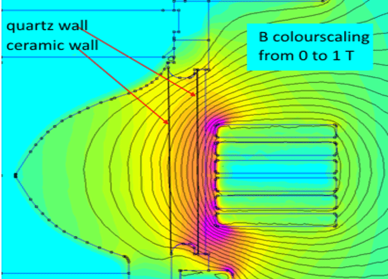 Figure 1
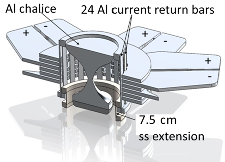 Figure 2
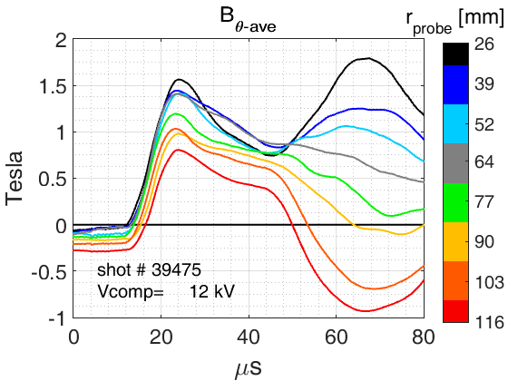 Figure 3
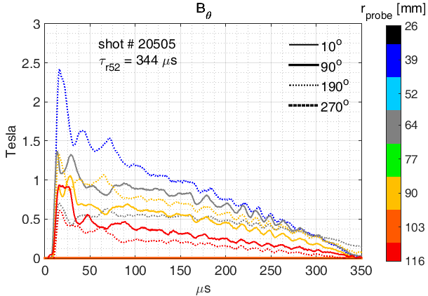 Figure 4
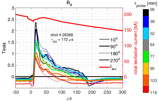 Figure 5
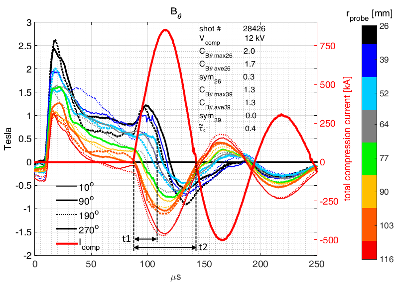 Figure 6
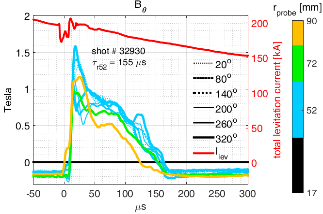 Figure 7
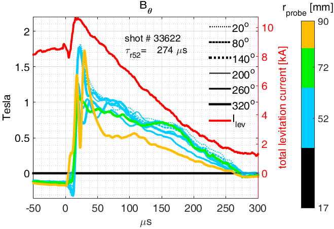 Figure 8
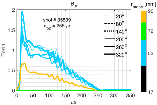 Figure 9
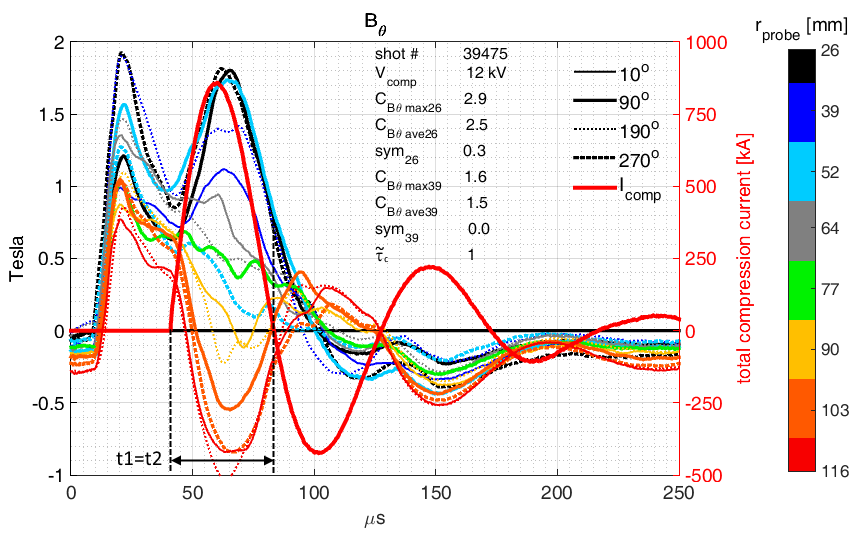 Figure 10
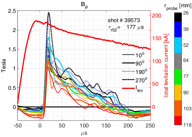 Figure 11
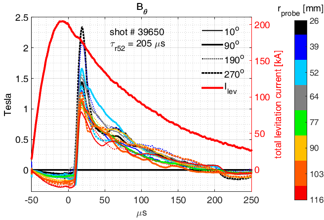 Figure 12
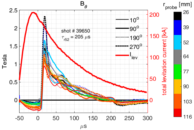 Figure 13
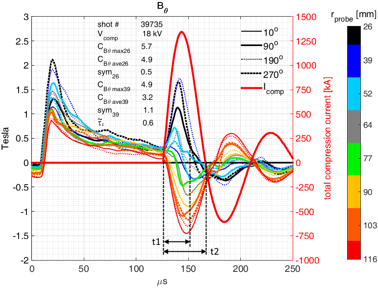 Figure 14
 Figure 15
 Figure 16
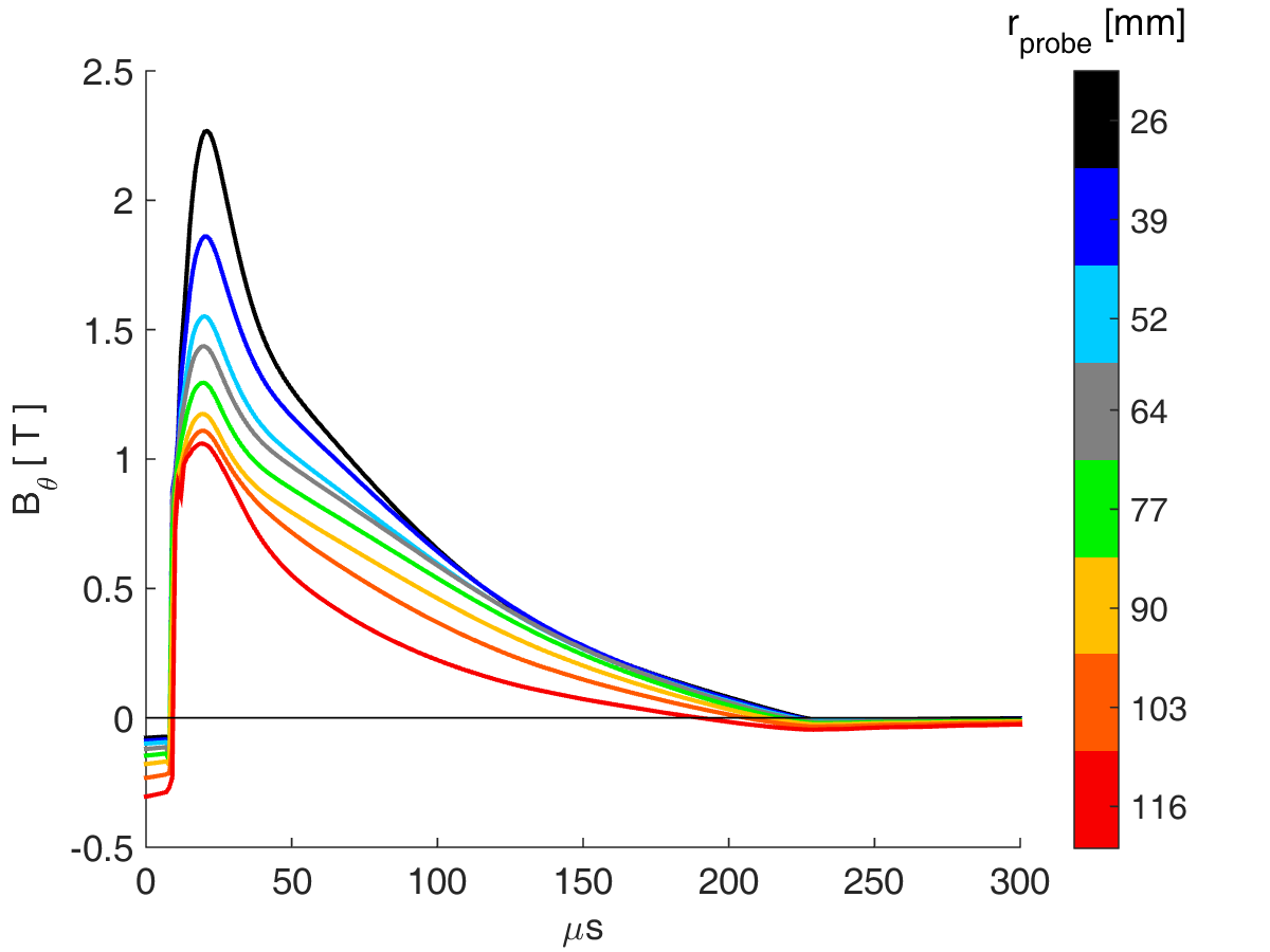 Figure 17
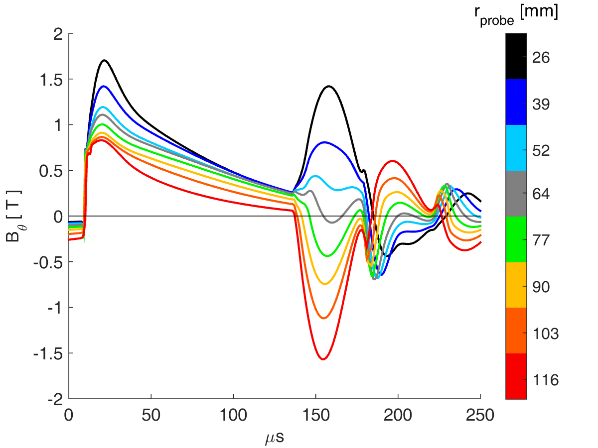 Figure 18
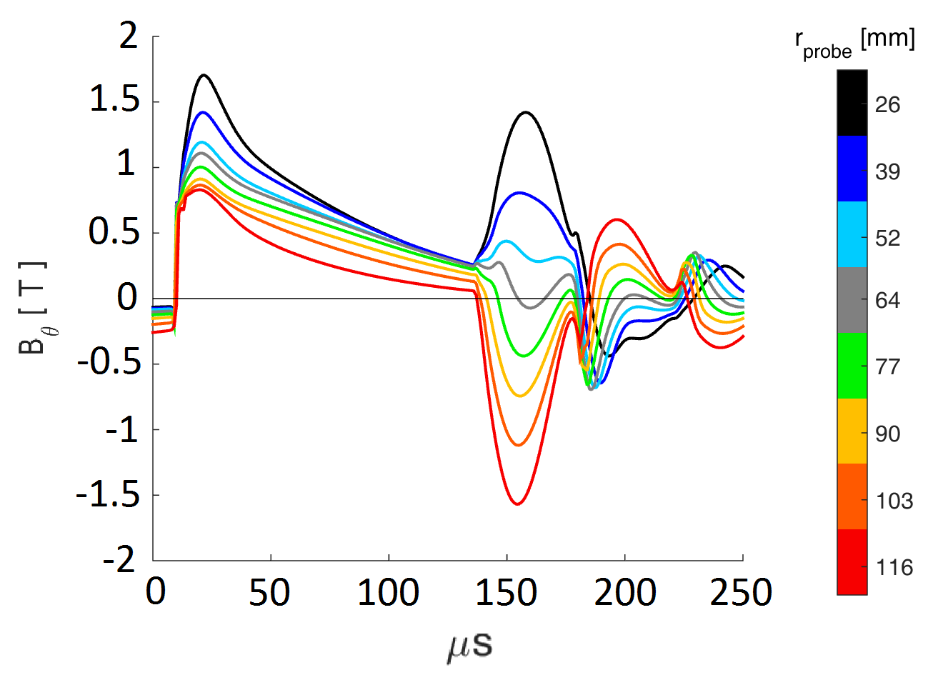 Figure 19
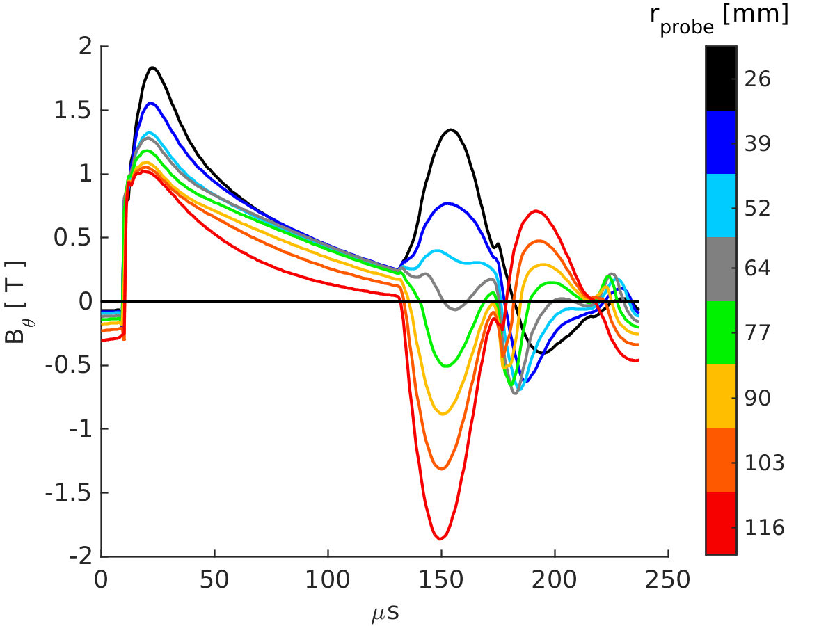 Figure 20
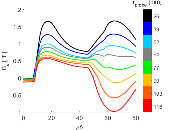 Figure 21
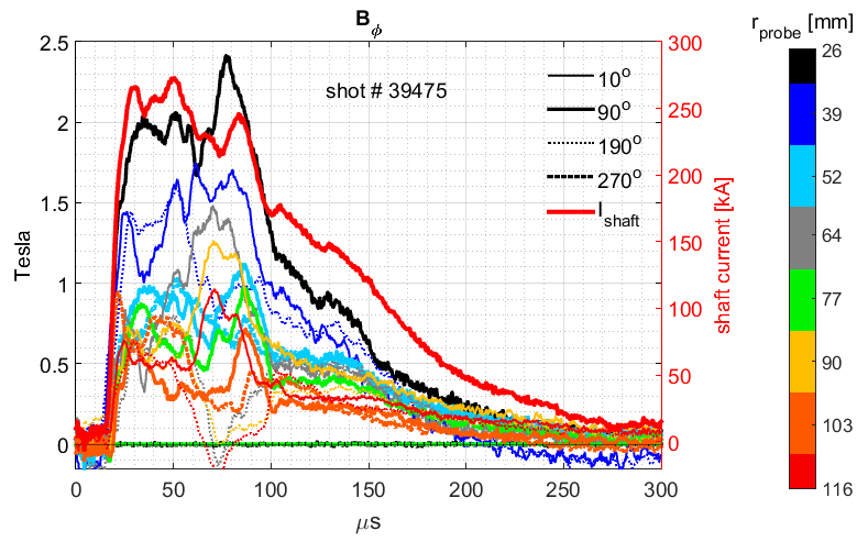 Figure 22
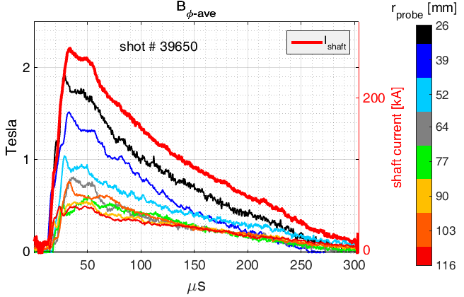 Figure 23
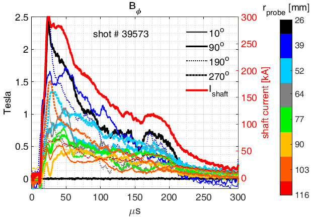 Figure 24
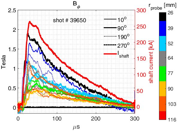 Figure 25
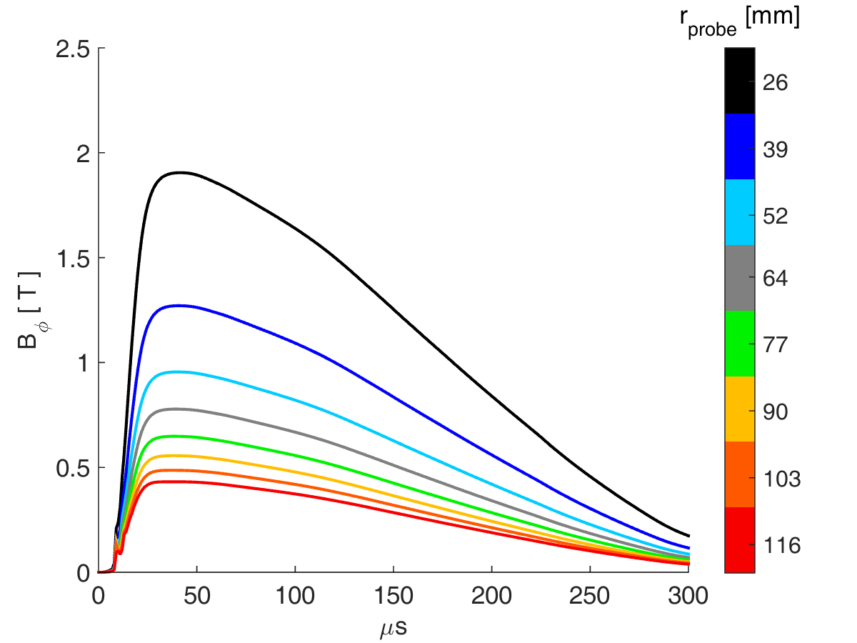 Figure 26
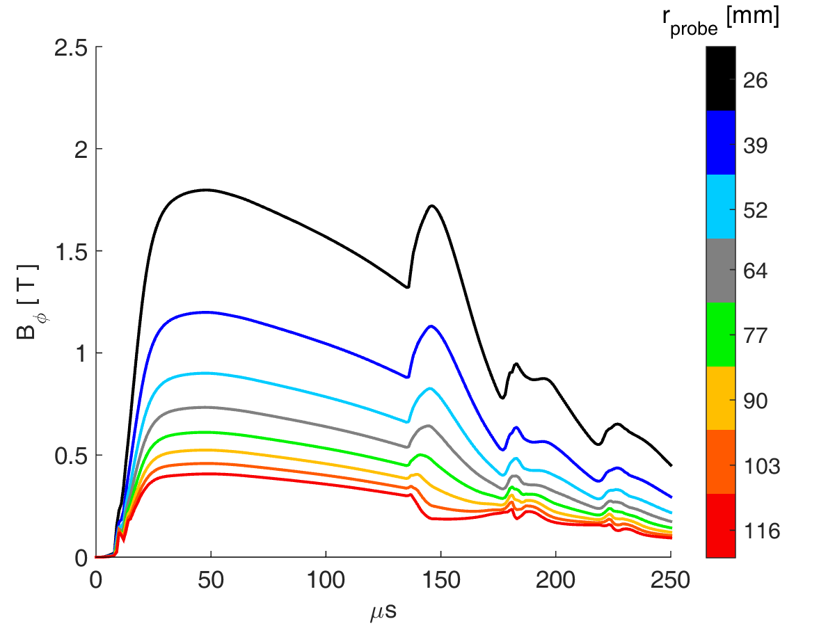 Figure 27
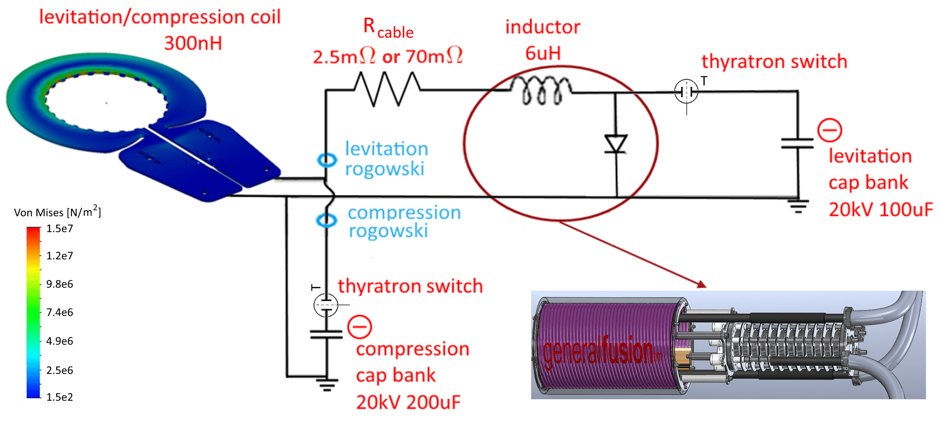 Figure 28
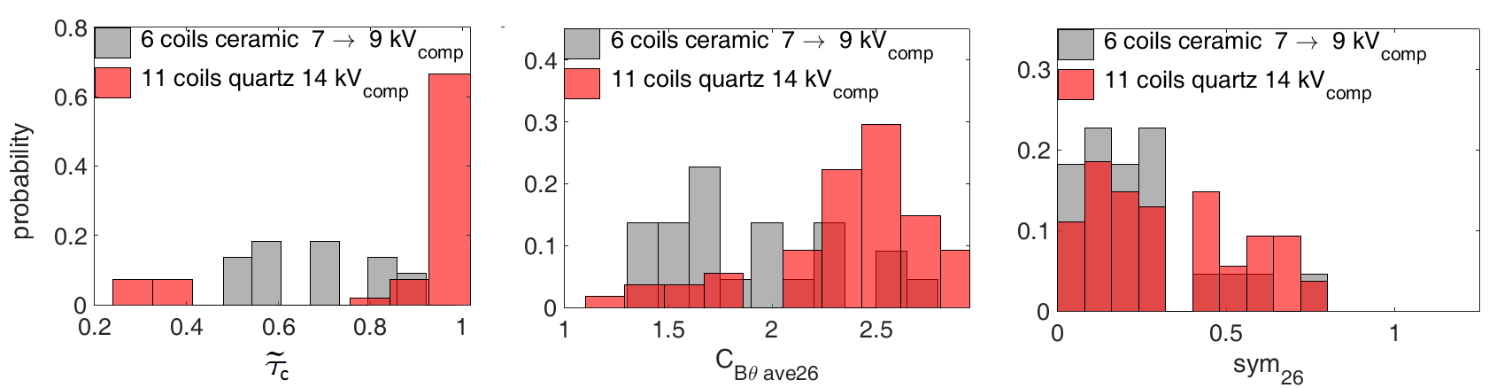 Figure 29
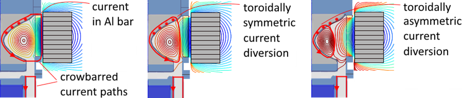 Figure 30
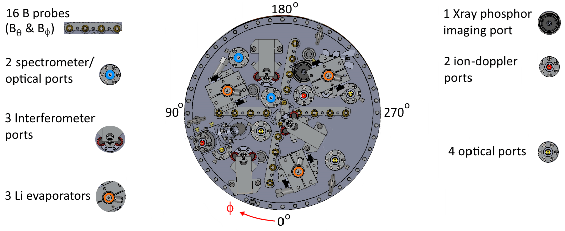 Figure 31
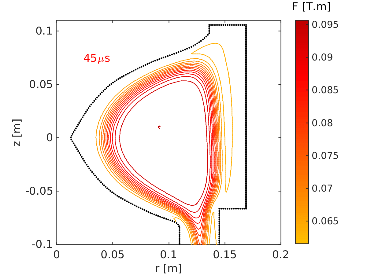 Figure 32
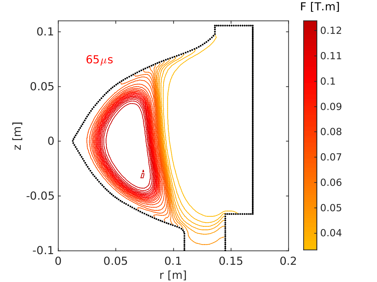 Figure 33
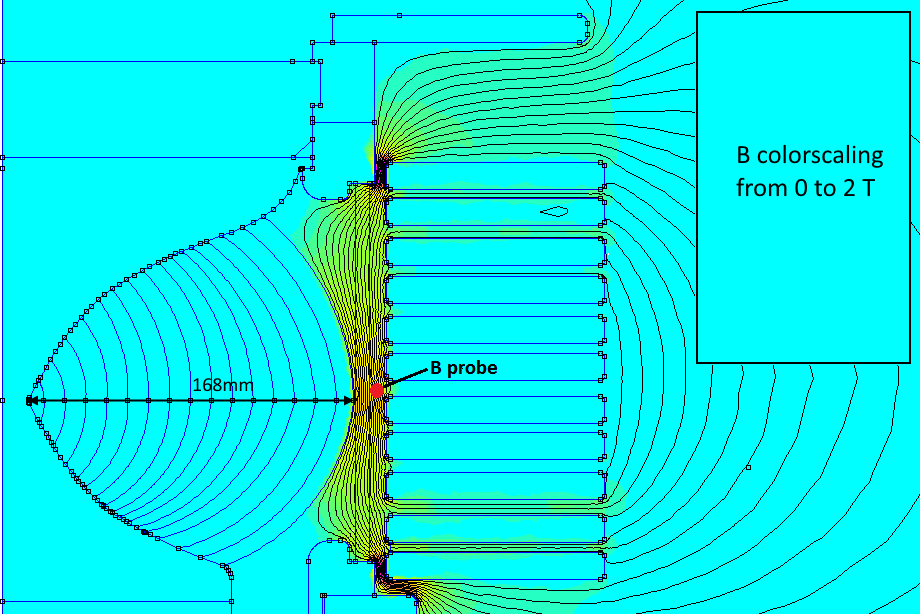 Figure 34
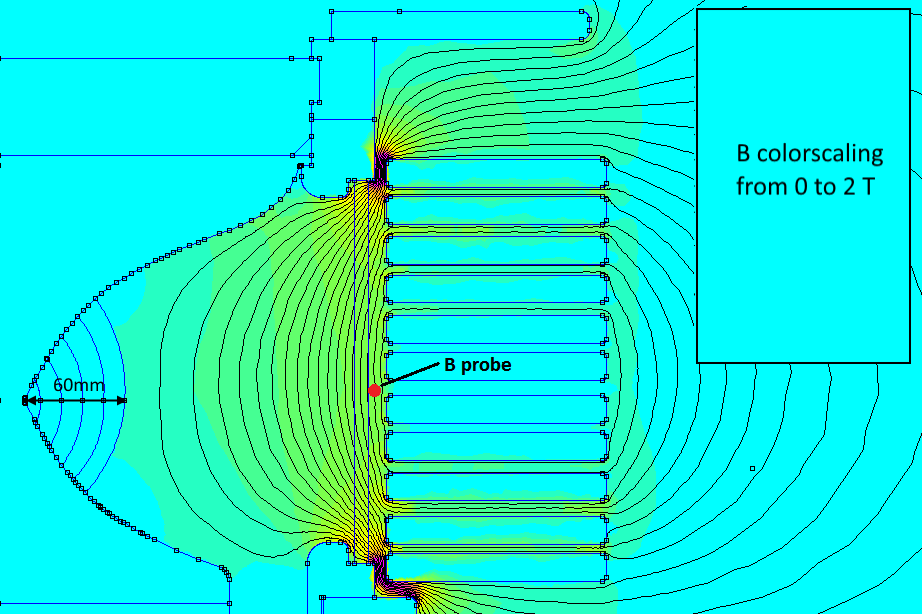 Figure 35
 Figure 36
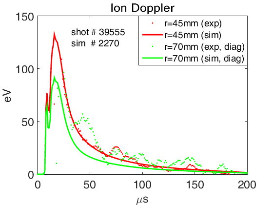 Figure 37
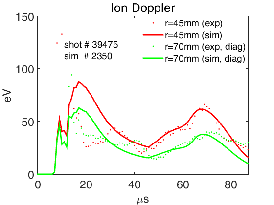 Figure 38
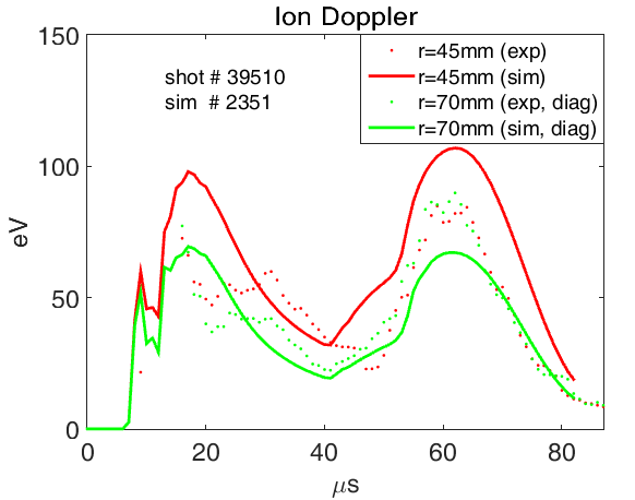 Figure 39
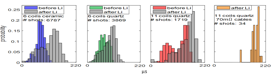 Figure 40
| (1) | Main coil is energised with steady state ( duration) current () | |
|---|---|---|
| (2) | s | Gas is injected into vacuum |
| (3) | Levitation banks, charged to voltage , are triggered | |
| (4) | s | Formation banks, charged to voltage , are triggered |
| (5) | Compression banks, charged to voltage , are triggered |
| [deg.] |
|---|
| parameter | |||||||
|---|---|---|---|---|---|---|---|
| scaling |
Peer Reviews
No public reviews on file for this paper yet. If you reviewed it on a platform where reviews are public (OpenReview, ICLR, NeurIPS, ICML), you can paste yours below so the community can read it here.
Videos
No videos yet. Explain this paper in a talk, walkthrough, or lecture? Add one.
Carl Dunlea1∗, Stephen Howard2, Wade Zawalski2, Kelly Epp2, Alex Mossman2,
Chijin Xiao1, Akira Hirose1
Magnetic Levitation and Compression of Compact Tori
Carl Dunlea1∗, Stephen Howard2, Wade Zawalski2, Kelly Epp2, Alex Mossman2,
Chijin Xiao1, Akira Hirose1
Abstract
The magnetic compression experiment at General Fusion was a repetitive non-destructive test to study plasma physics to Magnetic Target Fusion compression. A compact torus (CT) is formed with a co-axial gun into a containment region with an hour-glass shaped inner flux conserver, and an insulating outer wall. External coil currents keep the CT off the outer wall (radial levitation) and then rapidly compress it inwards. The optimal external coil configuration greatly improved both the levitated CT lifetime and the rate of shots with good flux conservation during compression. As confirmed by spectrometer data, the improved levitation field profile reduced plasma impurity levels by suppressing the interaction between plasma and the insulating outer wall during the formation process. Significant increases in magnetic field, density, and ion temperature were routinely observed at magnetic compression despite the prevalence of an instability, thought be an external kink, at compression. Matching the decay rate of the levitation coil currents to that of the internal CT currents resulted in a reduced level of MHD activity associated with unintentional compression by the levitation field, and a higher probability of long-lived CTs. An axisymmetric finite element MHD code that conserves system energy, particle count, angular momentum, and toroidal flux, was developed to study CT formation into a levitation field and magnetic compression. An overview of the principal experimental observations, and comparisons between simulated and experimental diagnostics are presented.
1University of Saskatchewan, 116 Science Pl, Saskatoon, SK S7N 5E2, Canada
2General Fusion, 106 - 3680 Bonneville Pl, Burnaby, BC V3N 4T5, Canada
*∗*e-mail: [email protected]
1 Introduction
General Fusion is developing a magnetized target fusion (MTF) power plant, based on the concept of compressing a compact torus (CT) plasma to fusion conditions by the action of external pistons on a liquid lead-lithium shell surrounding the CT [1, 2]. Magnetic confinement in self-organized compact toroids relies significantly on internal plasma currents. The CT can take on a range of magnetic profiles depending on boundary geometry and the amount of axial current running on a central shaft. The final magnetic structure of the CT can range from a spheromak up to spherical tokamak (ST) configuration with a higher safety factor profile. For MTF applications, the self-confining nature of the CT is essential because it enables CTs to be injected into the flux conserver of an MTF compression system, thereby physically separating and protecting the plasma formation system from the extreme and repetitive forces of a full power compression chamber. Understanding the thermal confinement physics associated with CTs during compression is critical to the MTF path forward. To study the plasma physics of CT compression, General Fusion has conducted a sequence of subscale experiments, refered to as Plasma Compression Small (PCS) tests [3]. In a PCS test, which takes place outdoors in a remote location, a CT is compressed by symmetrically collapsing the outer flux conserver with the use of chemical explosives. PCS tests are destructive, and therefore do not employ the full array of diagnostics used in CT formation and characterization experiments in the GF laboratory, and can only be executed every few months. However, in parallel to this, in the lab, an upgraded duplicate of the PCS plasma formation system called Super Magnetized Ring Test (SMRT) was configured to operate as a magnetic compression experiment, and ran from 2013 to 2016. It was designed as a repetitive, non-destructive test to study CT compression, in support of the PCS tests. A CT, with spheromak characteristics, is formed with a magnetized Marshall gun into a containment region with an hour-glass shaped inner flux conserver, and an insulating outer wall. Currents in external coils surrounding the containment region produce a magnetic field which applies a radial force on the plasma that "levitates" it off the outer wall during CT formation and relaxation, and then rapidly compresses it inwards.
With external levitation/compression coils, it was relatively straightforward to explore several different coil configurations. To accomplish fast compression while supporting large mechanical forces, the basic design of a stack of low-inductance single-turn coil plates was adopted (see figures 3, 5). Reduction of error fields was explored via variation of the geometry of current feed paths into each single turn plate, and also by departing from this fast pulse design to try a levitation-only 25-turn wound coil with higher inductance that had increased symmetry in order to see the effect of error fields on formation stability. Overall coil length and position was explored in a setup with a stack of six coil plates and another with a stack of eleven coil plates. Drive circuit parameters were also explored and we found optimum CT lifetime, and repeatability of good shots, when the decay of current in the levitation coil was tailored to match the typical decay time of the internal plasma current. The magnetic compression experimental campaign shed light on both fundamental plasma physics questions, as well as practical engineering concerns. One example of a practical lesson was the observation that interaction between plasma and the outer insulating wall during the CT formation could generate high levels of plasma impurities and radiative cooling under certain conditions. The wall material of high purity alumina ceramic was noticably less contaminating than the quartz wall that was tested. Analysis of the pulsed compression experiments indicated fast MHD instabilities during compression, likely related to the safety factor being too low.
Along with the experiments described in, for example, [4, 5, 6, 7], the experiment on which this work is based represents one of relatively few studies in which magnetic compression has been attempted on CTs produced by a magnetised Marshall gun. This is the first instance of magnetic compression by poloidal field on a stationary spheromak in a device without a co-axial railgun accelerator/compressor stage. In the past, mostly in the 1970’s and 1980’s, there were several theoretical and experimental studies looking at magnetic compression of conventional tokamak plasmas [8, 9, 10, 11, 12, 13, 14, 15], inductively formed spheromaks [16, 17, 18], and field reversed configurations [19, 20, 21].
Magnetic compression of spheromaks was the focus of the S-1 experiment [17, 18], in which a spheromak, with pre-compression major radius cm, and pre-compression minor radius cm, was inductively formed and then magnetically compressed using toroidal currents in coils located within the vacuum vessel. Pre-compression S-1 spheromaks had toroidal plasma current 200kA, corresponding to peak poloidal field 0.15T. A geometrical compression factor of 1.6, where and denote the pre-compression major and minor radii, while and denote the post compression radii, was achieved on the S-1 device [18], leading the researchers to classify the regime as constant aspect ratio [8] adiabatic compression. The availability of spheromak internal temperature, density, and magnetic field point diagnostics allowed the researchers to produce shot-averaged poloidal flux contours over the compression cycle, and enabled determination of the compression scalings for density, temperature and magnetic field, and comparison of the observed and predicted scalings. Fine spatial resolution of the magnetic field measurements allowed for experimental confirmation of several aspects of basic theory. For example, relaxation to the Taylor state, a process involving the anomalous conversion of poloidal to toroidal flux [27, 28], was observed during and after spheromak formation. Good spatial resolution of field measurements also enabled experimental confirmation of the approximate conservation of the individual fluxes, and of the absence of flux conversion during compression. Electron and ion temperatures were observed to increase at compression; peak rose from ~40eV to ~100eV with compression, and ion temperatures of up to 500eV were measured at compression.
The Adiabatic Toroidal Compressor (ATC) experiment [10, 11] (cm, cm, pre-compression), which was operated in the 1970’s, employed [8] adiabatic compression, in which scales in proportion to , and scales in proportion to . As in standard tokamaks, the vacuum vessel in enclosed by the toroidal field coils, but in the ATC, molybdenum rail limiters guide the plasma inwards at compression, which is activated by increasing toroidal current in the compression coils located outside the (electrically resistive) vacuum vessel, from 2 to 10kA over 2ms. Compression in , , , , , and was observed with scalings consistent with predictions for compression. The ATC compression mechanism is similar to the "radial magnetic pumping" scheme proposed in 1969 [29], in which it was suggested that a tokamak plasma would be maintained over several compression cycles, and that ions could be heated further at each compression. In [11], it was recommended that high frequency magnetic compression on ATC would be technically difficult, but that low frequency compression on a device, with dimensions increased to five to ten times those of ATC, might lead to ignition.
The scenario of attaining ohmic ignition through the combination of an ultra-low- discharge and adiabatic magnetic compression was explored in [12, 13, 14]. It was envisaged that with pre-compression conditions of eV and m*-3*, that the ignition parameters keV and m*-3* could, in principle, be achieved with .
TAE Technologies [20] and Helion Energy Inc. [21] have compressed FRCs to ion temperatures of several keV; a set of independently triggered formation and acceleration coils are used to form and merge two oppositely directed supersonic FRCs.
Merging-compression is a spherical tokamak (ST) plasma formation method that involves the merging and magnetic reconnection of two plasma rings, followed by inward radial magnetic compression of the resultant single torus to form a spherical tokamak plasma configuration. The initial tori are formed inductively around coils internal to the vacuum vessel, and the compression coils are also internal, an approach with some similarities to that developed on the S1 device. This ST plasma formation method has the advantage of eliminating the need for a traditional central solenoid - in an ST, space is limited in the central post and is inadequate for solenoids capable of inducing toroidal plasma currents in the MA range [22]. The merging phase leads to efficient transformation of magnetic to kinetic, then thermal energy (up to 15MW of ion heating power was recorded on on MAST), and also leads to a rapid increase of plasma current [22]. The merging compression ST formation method was first used on START [23, 24] in 1991, and then in MAST [25, 26], and is currently employed on the compact high field spherical tokamak ST40 at Tokamak Energy Ltd. [22].
This paper is arranged as follows. Section 2 is an overview of the magnetic compression device. Section 3 is focused on magnetic levitation of CTs. A description of various external coil configurations experimented with is presented in section 3.1. Principal results obtained in the study of magnetically levitated CTs will be presented, discussed, and compared with MHD-simulated diagnostics in section 3.2. A summary of the main findings from the study of levitated CTs, and comparisons of CT performance in the principal configurations tested constitutes section 3.3. Section 4 is focused on magnetic compression. The principal results from the magnetic compression experiments will be shown, discussed, and compared with simulation results in section 4.1. The mechanism behind the compressional instability that was routinely observed is discussed in section 4.2. A comparison of the performance of magnetically compressed CTs in the principal configurations tested is presented in section 4.3. The main conclusions from the levitation and compression experiment are outlined in section 5. A method developed to experimentally determine the outboard equatorial separatrix of levitated CTs is described, with results, in appendix A. In appendix B, the predicted adiabatic compression scalings for various parameters are compared with those obtained from MHD simulations.
2 Machine Overview
The overall structure and experiment design of the SMRT magnetic compression device can be seen in figure 1, including a schematic of the formation circuit and with CT and levitation (poloidal flux) contours from an equilibrium model superimposed. Measurements of formation current , and voltage across the formation electrodes are also indicated. Note that the principal materials used in the machine construction, and some key components, are indicated by the color-key at the top left of the figure. Apart from the inclusion of the levitation/compression coils and the insulating tube around the CT containment region, the machine is identical to the standard pre - 2016 General Fusion MRT (Magnetized Ring Test) plasma injectors, which had an aluminum outer flux conserver in place of the insulating tube. The sequence of machine operation is as follows:
To better illustrate the sequence of operation, contours from an MHD simulation of the magnetic compression experiment are shown in figure 2. As described separately in [30, 31], an energy, particle, and toroidal flux conserving finite element axisymmetric MHD code was developed to study CT formation into a levitation field, and magnetic compression. The Braginskii MHD equations with anisotropic heat conduction were implemented. To simulate plasma / insulating wall interaction, we couple the vacuum field solution in the insulating region to the full MHD solution in the remainder of the domain. A plasma-neutral interaction model including ionization, recombination, charge-exchange reactions, and a neutral particle source, was implemented in order to study the effect of neutral gas in the gun on simulated formation [32]. In figure 2, note that contours represent poloidal field lines, and that the vertical black line at the top-right of the figures at represents the inner radius of the insulating wall. Vacuum field only is solved for to the right of the line, and the plasma dynamics are solved for in the remaining solution domain to the left of the line. The inner radius of the stack of eleven levitation/compression coils (which are not depicted here) is located at the outer edge of the solution domain, at . Simulation times are notated in red at the top left of the figures. Note that the colorbar scaling changes over time; decreases slowly over time as the CT decays, while min increases as the levitation current in the external coils decays, and then drops off rapidly as the compression current in the external coils is increased, starting at in this simulation. At time the stuffing field () due to currents in the main coil fills the vacuum below the containment region, and has soaked well into all materials around the gun, while the levitation field fills the containment region. Simulated CT formation is initiated with the addition of toroidal flux below the gas puff valves located at m; initial intra-electrode radial formation current is assumed to flow at the z-coordinate of the valves. As described in detail in [30, 31], toroidal flux addition is scaled over time in proportion to . Open field lines that are resistively pinned to the electrodes, and partially frozen into the conducting plasma, have been advected by the force into the containment region by ( is the radial formation current density across the plasma between the electrodes, and is the toroidal field due to the axial formation current in the electrodes). By , open field lines have reconnected at the entrance to the containment region to form closed CT flux surfaces. At these early times, open field lines remain in place surrounding the CT. Compression starts at and peak compression is at . The CT expands again between and as the compression current in the external levitation/compression coils decreases. Note that at s, magnetic compression causes closed CT poloidal field lines that extend down the gun to be pinched off at the gun entrance, where they reconnect to form a second smaller CT. Field lines that remain open surrounding the main CT are then also reconnectively pinched off, forming additional closed field lines around the main CT, while the newly reconnected open field lines below the main CT act like a slingshot that advects the smaller CT down the gun, as can be seen at .
A pulse-width modulation system was used for current control in the main coil circuit. The working gas was typically or , with valve plenum pressure , and optimal vacuum pressure . The formation capacitor bank ( capacitors in parallel) drives up to 1MA of current, with a half period of (see figure 1 inset). The original machine configuration had six levitation/compression coils, with each coil having its own levitation and compression circuit. The levitation bank consisted of two capacitors in parallel for each coil, and there were four of these capacitors in parallel for each coil for the compression bank.
The circuit for one of the single-turn levitation and compression coils is depicted in figure 3. Each coil (or coil-pair in the case of the configuration with 11 coils) had a separate identical circuit. Unlike the crowbarred levitation currents, the compression currents are allowed to ring with the capacitor discharge. Typical levitation and compression current waveforms are shown in figures 7 and 16 (right axes).
A schematic of the machine headplate (top view) indicating the principal diagnostics and lithium evaporator ports is shown in figure 4(a). Lithium coating on the surfaces of the containment region was applied routinely as a gettering agent, and resulted in levitated CT lifetime improvements of up to 70%, depending on the insulating wall material, as outlined in section 3.3. Figure 4(b) depicts the tungsten-coated aluminum inner flux-conserver, indicating the locations of some of B-probe ports and the lines-of-sight for the ion Doppler and interferometer diagnostics. For ease of depiction, the ion Doppler/interferometer chords are shown to be located on the same poloidal plane. Line-averaged electron density was obtained along chords at and using dual nm and nm He-Ne laser interferometers. Dual wavelength Michelson-type interferometers were used to enable compensation for errors due to machine vibration during a shot. Note that the plasma-traversing beam crosses through the plasma twice. Retroreflectors positioned in the base of the inner flux conserver reflect the beam back up through the plasma. The reference beam is directed along a path of equal length in ambient air. An indication of ion temperature, along the vertical chord at and the diagonal chord with its upper point at , was found from Doppler broadening of line radiation from singly ionized Helium (He II line at 468.5nm). Visible light emission is recorded by two survey spectrometers which have variable exposure durations, and by six fiber-coupled photodiodes that record time-histories of total optical emission.
Two magnetic probes, for recording poloidal and toroidal field, were located at the closed ends of each of sixteen thin-walled stainless steel tubes embedded in axially directed holes in the inner flux conserver. The coordinates of the probes, where is defined as being at the machine axis, are:
3 Magnetic Levitation
3.1 Overview of external
coil configurations
Figure 5(a) indicates, for the original configuration with six coils, the inner flux conserver, coils, stainless steel extension, and aluminum return-current bars that carry axial current outside the insulating wall. The inner radii of the original ceramic (alumina - ) wall, and of the quartz (silica - SiO2) wall that was tested later, are shown in 5(b). This is an output plot from the open-source FEMM (Finite Element Method Magnetics) program[33], with per coil and an input current frequency of Hz. Contours of , poloidal levitation flux, are shown, with the plot colour-scaling being proportional to FEMM models alternating currents as sinusoidal waveforms in time, so we chose s to be the quarter- period, giving a frequency of Hz. In the configuration with six coils, it was found that CT lifetimes could be increased by by firing the levitation capacitors at , well before firing the formation capacitors. This allows the levitation field to soak into the stainless steel above and below the wall, resulting in line-tying (field-line pinning) - magnetic field that is allowed to soak into the steel can only be displaced on the resistive timescale of the metal, which is longer than the time it takes for the CT to bubble-in to the containment region. Note that the principal materials used in the construction of the magnetic compression machine are indicated in figure 1. As confirmed by MHD simulations [31], this line-tying effect is thought to have reduced plasma-wall interaction and CT impurity inventory by making it a little harder for magnetised plasma entering the confinement region to push aside the levitation field. FEMM models were used to produce boundary conditions for , pertaining to the peak values of toroidal currents in the main, levitation, and compression coils at the relevant frequencies, for MHD and equilibrium simulations. For MHD simulations, boundary conditions for and are scaled over time according to the experimentally measured waveforms for and .
The high stainless steel extension indicated in figure 5(a) was an addition to the original configuration that also helped reduce the problem of plasma-wall interaction. In the original design without the extension, the ceramic insulating outer wall extended down an additional 7.5cm. With the original levitation field profile from six coils, and without the extension, levitated CTs were short-lived, up to s as determined from the poloidal B-probes embedded in the aluminum inner flux conserver at (see figures 1 and 4(a)), compared with over s for non-levitated CTs produced in MRT injectors with an aluminum outer flux conserver. CT lifetime was increased, up to s, with the addition of the steel extension. The extension mitigated the problems of sputtering of steel at the alumina/steel lower interface, and of plasma interaction with the insulating wall during the formation process.
An insulating wall with larger internal radius was tested (original alumina tube with was replaced with a quartz tube with ). The resistive part of is , where is the elliptic Laplacian-type operator used in the Grad-Shafranov equation, and is the magnetic diffusivity, so CT lifetime should scale approximately with , where is the characteristic length scale associated with the CT. The radius of the inboard wall at the inner flux conserver waist at is . The minor CT radius for a given would be approximately , so assuming that , we have . From this rough estimate, for a given , an increase from s to s was expected with the transition to the larger radius quartz tube. However lifetime decreased noticeably (s to s) with the transition, so that in terms of CT lifetime, plasma interaction with quartz was almost as bad as with alumina. The quartz wall led to more plasma impurities (see section 3.3), and consequent further radiative cooling, and therefore an increased rate of resistive decay.
In the 6-coil configuration, the longest-lived CTs were achieved at generally low settings for , , and (note that for optimal settings, these parameters, defined in table 1, scale with one another), resulting in low-flux CTs. For example, would typically have been and compared with and for best performance on standard MRT machines. Note that kV corresponds to a peak formation current of kA, while A corresponds to a gun flux of around 12mWb. Increasing these parameters on the magnetic compression injector in the 6-coil configuration led to increased impurity levels and degraded lifetime further.
After CT formation and relaxation, it was usual, with the standard MRT machines from around 2013 onwards, to observe magnetic fluctuations with toroidal mode number on the measured signals, as determined by phase analysis of the signals from probes located at the same radius apart toroidally (see table 2). These fluctuations are evidence of coherent CT toroidal rotation, and were absent on shots taken on the magnetic compression device. There was concern that rotation could be impeded by mode-locking caused by toroidal asymmetry in the levitation field, introduced by the gaps in toroidal levitation current associated with the single-turn coils. A set of six new coils (coil outline is depicted in figure 3), which reduced the original field error by a factor of , was manufactured. Also, a 25-turn, high inductance (H) coil was experimented with - this reduced the original field error by a factor of Due to its long s current rise time, and inadequate structural resistance against forces, the 25-turn coil could be used only for CT levitation (in connection with a single levitation circuit), and not for compression. The coil was made with a height that extended all the way along the insulating wall, closing the gaps outboard of the wall that were present above and below the 6-coil stack. It was thought that the presence of the gaps facilitated the process by which magnetised plasma entering the confinement region at formation can push aside the levitation field and interact with the insulating wall, sputtering impurities into the plasma.
It turned out that levitation field asymmetry associated with the original single-turn coils was not a problem at the level of performance achieved. At the settings for low-flux CTs, no improvement in CT lifetime or symmetry was seen with either the new set of discrete coils or the 25-turn coil, and there was no additional evidence of CT rotation, nor evidence that a mode-locking issue had been alleviated. Movement of filamentary structures observed with X-ray phosphor imaging indicated the likelihood of CT rotation, but couldn’t confirm it. Coherent CT rotation was confirmed later in the experiment; fluctuations regularly appeared on the traces when additional toroidal field was included with the use of crowbarred formation current. The fluctuations observed on signals with standard MRT machines may be connected with internal reconnection events that occurred upon exceeding a threshold in CT temperature. The first appearance of the fluctuations on MRT machines was in 2013, when titanium gettering was first experimented with. Back in 2013, titanium gettering led to CT lifetime increases of up to , to , and an increase in electron temperature, as determined with Thomson scattering, from near the CT core.
As a result of the modification of the levitation field profile, the 25-turn coil allowed for the production of high flux levitated CTs, with a corresponding improvement in lifetime. At and , best CT lifetimes with the quartz insulating wall improved , from s (low flux CTs with 6 coils) to s. With a single levitation circuit, the 25-turn coil also facilitated the optimization of circuit parameters, and it was found that CT lifetime and repeatability of good shots (long CT lifetime) could be improved by adding resistance to the circuit in order to match the decay rate of the levitation current to that of the CT current.
The 11-coil configuration consisted of 5 coil pairs and one single coil, and approximately reproduced the levitation field profile of the 25-turn coil, allowing for formation and compression of higher-flux CTs with correspondingly increased lifetimes. Each pair was assembled using one of the original coils, clamped together in parallel with one of the newer coils that were designed to increase toroidal symmetry in the levitation/compression field. The remaining newer coil was included on its own, positioned 3rd from the bottom of the 11-coil stack, to further increase the field at the top and bottom of the wall.
The 11-coil stack installed on the machine is shown in figure 6(a)
- the single coil is visible on the lower right. Each coil/coil-pair is connected to its own levitation circuit via the two outer co-axial cables in the cable connecting bracket attached to the coil/coil-pair. One of the six brackets can be seen in the upper left foreground. Each of the inner four co-axial cables in each bracket links individually to a compression capacitor and thyratron switch. Figure 6(b) shows a FEMM output plot of the levitation field for the 11-coil setup with per coil and a solution frequency of kHz, corresponding to the experimentally determined optimal delay of s between the firing of the levitation and formation capacitor banks. Note that the strategy used with the 6-coil configuration of increasing to reduce plasma/wall interaction was not required with the 11-coil configuration.
3.2 Overview of results and comparison with simulations - CT levitation
3.2.1 Magnetic field measurements
Measurements of and for two shots taken in the 11-coil configuration, with different cable resistances (denoted as in the levitation/compression circuit schematic in figure 3), is shown in figure 7. As indicated in table 2, there are sixteen magnetic probe heads located in the inner flux conserver
- eight of these are located at four different radii (, and 116mm) at toroidal angle and , and there are an additional eight probes at (, and 103mm) at and . Magnetic probe signals are colored by the radial coordinates of the probe locations, with toroidal coordinates of the probe locations denoted by linestyle, as denoted in the plot legends. CT lifetime is gauged using the metric (indicated in figures 7(a) and (b)), which is the time at which the average of the poloidal field measured at the two probes at 52mm crosses zero. Note that is the field component parallel to the inner flux conserver surface in the poloidal plane. Total levitation current, measured with Rogowski coils, is also indicated in figures 7(a) and (b) (thick red lines, right axes) for the two shots. s for these shots, so with a current rise time of s in the levitation coils, the poloidal levitation field measured at the probes reaches its maximum negative value at s. Formation capacitors are fired at s, and (referring to figure 2) it takes s for the gun (stuffing) flux to be advected up to the probe locations. The stuffing field has opposite polarity to the levitation field. Over the next several tens of s, during and after reconnection of poloidal field to form closed flux surfaces, the CT undergoes Taylor relaxation, involving conversions between poloidal and toroidal fluxes. The CT shrinks and is displaced inwards by the levitation field as the CT currents and fields decay resistively. As the CT decays, starting at the outer probes and progressing inwards towards the inner probes, the CT field measured at the probes is once again replaced by the levitation field. After s (figures 7(a) and (b)), the field measured at all the B probes is the levitation field. Note that, when levitation field is being measured at the probes, that is larger at the outer probes, due to the scaling of levitation field with levitation current in the external coils. On the other hand, when CT field is being measured at the probes, is larger at the inner probes, due to the scaling of CT field with CT flux - poloidal field lines are bunched together progressively more at smaller radii.
The shots referred to in figures 7(a) and (b) were both at , , additional settings included for shot 39573, and for shot 39650. To achieve approximately the same levitation current, was increased for shot 39650 to compensate for the additional cable resistance. It can be seen how the decay rate of approximately matches that of the CT toroidal current (as determined by positive ) with a cable replacing the original pair of cables in parallel ( total ) between the main holding inductor and coil in each levitation circuit. A much higher rate of "good" shots, smoother decays of and (less apparent MHD activity), and a lifetime increase generally of around , was observed with the cables in place. With the low resistance cables, the CT is decaying far faster than the levitation field, so that it is being compressed (without firing the compression banks) by the levitation field more and more as decreases. By matching the levitation field decay rate to that of the CT currents, the CT is allowed to retain the size that it would have if it was being held in place by field due to eddy currents induced in an outboard flux-conserver, instead of by an outboard levitation field. It can be seen how the CT is being displaced from larger radii much faster in shot 39573, compared with shot 39650, in which decay rate matching was implemented. In shot 39573, the CT has been displaced inwards beyond the probe at by s, when the signal from the 116mm probe goes negative, but this displacement is delayed until s, in shot 39650. As described in appendix A, a method was developed to experimentally measure the outboard CT separatrix using data from a set of eight magnetic probes located on the insulating wall. This method allows for time-resolved determination of the outboard CT separatrix at eight equally spaced toroidal angles, and comparison of this between configurations.
Referring again to figures 7(a) and (b), note that in shot 39573, CT poloidal field at the inner probes collapses rapidly to zero at s, whereas the decay is much smoother in shot 39650 - this sudden collapse is due to the compressional instability that will be discussed in section 4.
With reference to figures 7(c) and (d), , the toroidal field measured at the probes, is due to poloidal shaft current in the inner flux conserver. Shaft current is induced to flow in conducting material surrounding the CT as the system tries to conserve the toroidal flux introduced at CT formation, and continues to decay away resistively for several tens of microseconds after the CT currents have decayed. The current path includes the inner flux conserver walls, aluminum bars (indicated in figure 5(a)), and a path through ambient plasma in the gap below the CT between the bottom of the inner flux conserver and the outer electrode. (thick red traces in figures 7(c) and (d)) is calculated from using Ampere’s law. As the CT shrinks due to compression, increasing proportions of poloidal shaft current can divert from the initial paths in the aluminum bars, and flow through the ambient plasma outboard of the CT. This will be clarified in section 4. Shaft current increases when it flows along the reduced inductance path through the ambient plasma. There is evidence in figure 7(c) of mild magnetic compression by the levitation field starting at around s on shot 39573 (with the low resistance cables). This is evident from the overall rise in shaft current at s, and from the rise at the probes, particularly at the and probes. This unintentional compression is absent with the implementation of decay-rate matching, as seen in figure 7(d) for shot 39650.
Figures 8(a) and (b) show recorded at the probe locations from MHD simulations in which the boundary conditions pertaining to the levitation field were evolved over time according to the experimentally measured waveforms for , which depend on the resistance of the cables in the levitation circuit, as indicated in figure 7(a) and (b) (right axes). Comparing the traces in figures 7(a) and 8(a), it can be seen how the comparison is qualitatively good up until around s, when the compressional instability, which is not captured by the 2D MHD dynamics, causes the CT to be extinguished rapidly. The comparison in figures 7(b) and 8(b) remains good at all times, as the compressional instability did not arise in the case with decay rate matching.
Experimentally measured for shot 39650, taken in the eleven coil configuration with cable resistance, is shown in figure 9(a). For ease of comparison, the toroidal averages of the toroidal field traces measured at the two probes 180o apart at each of the eight radii, at which the magnetic probes in inner flux conserver are located, are shown here. With cable resistance, the compressional instability that was routinely observed on levitation-only shots with the cable resistance is not observed, so the simulated toroidal field, shown in figure 9(b), is a good match to the experimental measurements. Shaft current is not used as an input to the simulation, rather it arises naturally in simulations as a consequence of induced wall-to-wall currents that act to conserve total toroidal flux (see [30, 31] for details).
3.2.2 Ion temperature and electron density
measurements
Profiles of electron density and neutral particle density from an MHD simulation (# 2270) [30, 31, 32] at early time (s) during the formation of the CT are shown in figures 10(a) and (b). At this time, plasma has been advected up the Marshall gun and is entering (bubbling into) the CT containment region, along with partially frozen-in open stuffing field that is resistively pinned to the inner and outer electrodes further down the gun at m, and is displacing the levitation field in the containment region. The vertical blue, red and green chords in figure 10(a) represent the lines of sight of the interferometer measurements ( figure 4(b)). Initial plasma fluid density (note we use a single fluid MHD, but partition the energy equation into ion and electron components) is concentrated around the gas valves down the gun at m. The initial neutral fluid density distribution, also centred around the gas valves, extends further than the initial plasma fluid density distribution, so that a front of neutral fluid precedes the plasma as it is advected into the containment region.
Figure 10(c) shows contours of from the same simulation at s. Levitation field continues to be displaced in the containment region. Figures 10(d), (e) and (f) show contours of and at the same time. Thermal diffusion is anisotropic in this simulation, with constant coefficients . In general, upper bounds on the parallel ion and electron thermal diffusion coefficients are imposed by the minimum practical timestep
- an explicit timestepping scheme is used. The perpendicular coefficients are chosen so as to match the decay rate of CT currents and fields to experimentally indicated rates - radiative cooling due to the presence of high impurities in the plasma is not modelled directly - instead, enhanced perpendicular thermal diffusion is used as a proxy for this cooling. It can be seen how temperature is equilibriating along field lines even at these early times, and, as a consequence of ionization, neutral density is reduced at regions of high electron temperature.
As indicated in figures 10(g) and (h), high plasma-fluid velocities during the simulated formation process, largely due to rapid upward advection, and due to jets associated with magnetic reconnection of CT polodal field near the entrance to the containment region, lead to significant levels of ion viscous heating. The chords along which simulated ion Doppler measurements are taken, for comparison with experimental measurements (see figure 4(b)), can be seen in figure 10(h).
Figures 11(a) and (b) indicate the agreement between experimentally measured and simulated ion temperature and electron density. These simulated diagnostics are the corresponding line-averaged quantities along the chords indicated in figures 10(h) and (a) respectively. Note that the diagonal green coloured chord indicated in figure 10(h) has its lower point at mm. With reference to data presented in [34, 35], a maximum error in the temperature measurement (He II line at 468.5nm) due to density broadening has been evaluated as around 13eV for the peak density of 1.2m*-3*, and the error falls off in proportion to . The interferometer looking along the chord at mm (figure 4(b)) was not working for this shot, so this measurement has not been included here.
3.3 Main points - CT levitation
Normalised histograms comparing total spectral power recorded with spectrometer 1 (the spectrometer located at larger radius, depicted in figure 4(a)) for the 6-coil and 11-coil configurations with the quartz wall, are shown in figure 12. Data from 400 pre-lithium shots for each configuration, all with spectrometer exposure from [math] to s, is included. The validity of the data was verified by comparing the total spectral power recorded with the measured intensity of plasma optical emission at the same location as the spectrometer (the spectrometers shared ports with optical feedthroughs), and finding a good correlation. Even at increased formation voltage, total spectral power is around four times lower with eleven coils. This is particularly unusual because on a given configuration, it’s expected that higher formation current leads to increased ablation of electrode material and consequently increased impurity levels and total spectral power. The 11-coil setup reduced impurities and the associated energy losses due to line radiation because it reduced the level of interaction between plasma and the outer insulating wall during the bubble-in process, and the benefit from the reduction of plasma-insulating wall interaction was more significant than any impurity level augmentation caused by increased plasma-electrode interaction.
MHD simulations confirm the reduction of plasma-wall interaction with the eleven coil configuration, as indicated in figure 13. In figure 13(a), the stack of six coils is partly located in the blank rectangle on the right, centered around , and extends off further to the right (not shown). The region above, below, and just to the left of the coil-stack represents the air around the stack. The vertical black line at represents the inner radius of the insulating wall, and the outer radius of the insulating wall at is not indicated. In figure 13(b), the stack of eleven coils extends all the way from the top to the bottom of the insulating wall, and the inner radius of the coil stack is the same as that for the six coil stack. In both cases, as described in [30, 31], only , which determines the vacuum poloidal field, is evaluated in the insulating region to the right of the inner radius of the insulating wall. The solution for is coupled to the full MHD solution in the remainder of the domain. To maintain toroidal flux conservation, boundary conditions for , which has a finite constant value in the insulating wall and is zero outside the current-carrying aluminum bars depicted in figure 5(a), are evaluated and applied to the part of the boundary representing the inner radius of the insulating wall. Both simulations have boundary conditions for and from FEMM models, pertaining to A, and with the total levitation current such that is approximately the same for each configuration. Figure 13(a) indicates how poloidal field penetrates the insulating wall during the bubble-in process in the six coil configuration. In practice, ions streaming along and gyro-rotating around the field lines would then sputter insulating material into the plasma, leading to impurity radiation and radiative cooling, with consequent increased resistivity and reduced CT magnetic lifetimes.
As indicated in the normalised histograms in figure 14, pre-lithium CT lifetimes were longer with the ceramic wall despite the smaller volume. Lithium gettering was very effective on the ceramic wall ( lifetime increase), but not so effective on quartz ( lifetime increase). Lifetime increased significantly with the 11-coil configuration. The "double-Gaussian" shape of the (before Li) distribution for eleven coils may be due to the % of shots taken in that configuration in suboptimal machine-parameter space ( values of , and ) that were rapidly explored in the last days of the experiment in new configurations such as without levitation inductors, with additional crowbarred sustain current ( addition formation current with a decay time of ), and with passive or open-circuited levitation/compression coils. Note that of the shots from which data is taken for this levitated CT lifetime comparison, only 34 shots in the best of the configurations tested - eleven coils with cables - are shown because the 11-coil configuration was explored rapidly in the days before the experiment was decommissioned. The repeatability of good shots was significantly improved in that configuration.
Poloidal field traces for the six principal configurations tested are shown in figure 15. Note that the magnetic probes are located at radial and azimuthal coordinates different to those listed in table 2 for the configurations relevant to figures (b), (c) and (e). Note that not all of the magnetic probes were functioning in some shots, for example the signals relevant to the probes at mm and mm have been zeroed out in figure 15(e). Comparing figures 15(a) and (b), and noting, as outlined in section 3.1, that a 50% increase in CT lifetime was expected with the switch to the larger internal radius insulating tube, it can be seen how quartz was significantly worse than ceramic as a plasma-facing material. For these two shots, was s - as mentioned in section 3.1, the strategy of allowing the levitation field more time to soak into the steel above and below the insulating wall led to slightly increased CT lifetimes on the 6-coil configurations.
With CT lifetimes of up to s, the longest-lived levitated CTs were produced with the 25 turn coil configuration (figure 15(c)). The eleven coil configuration, with a field profile similar to that of the 25-turn coil setup, also enabled the production of relatively high-flux CTs with correspondingly increased lifetimes (figure 15(d)). In general, the recurrence rate of good shots in the 25-turn coil configuration was poor compared with that in the 11-coil configuration. However, it remains unclear why the longest-lived CTs produced with the 25-turn configuration outlived those produced in the 11-coil configuration. The most likely explanation is connected to the fact that the 25-turn coil extended farther above and below the insulating wall than the stack of eleven coils. It may be that the increased levitation field, relative to that for the 11-coil configuration, at the top and bottom of the insulating wall, played a key role. At low formation settings, without addition levitation circuit series resistance, levitated CT lifetimes in the 25-turn configuration were comparable to those in both the 11-coil and 6-coil configurations. It is clear that the feature shared by the 25-turn and 11-coil configurations, of closing the gaps that remained above and below the coil stack in the 6-coil configurations, was responsible for enabling the formation of high flux CTs with correspondingly increased lifetimes, and that the unconfirmed mechanism that enabled (occasional) even better performance in the 25-turn configuration was also effective only at high formation settings. Another possible explanation concerns the ratio of the coil inductance to the levitation circuit holding inductance, which was increased from for the 11-coil configuration to for the 25-turn coil. When conductive plasma enters the pot (confinement region) it reduces the inductance of the part of the levitation circuit that includes the levitation/compression coil and the material that the coil encompasses. The levitation current increases when the inductance is reduced as plasma enters the pot. If the percentage rise of the levitation current is increased, by increasing the ratio , it means that levitation current prior to plasma bubble-in can be minimised. This reduction in reduces the likelihood that the levitation field will be strong enough to partially block plasma entry to the pot, while still allowing the field that is present, when the plasma does enter, to be strong enough to levitate the plasma away from the insulating wall. Comparing figures 15(c) and (d), it can be seen how the levitation current increases significantly at bubble-in for the 25-turn coil only. FEMM models indicate that the levitation fluxes found to be optimal at moderately high formation settings for the 25-turn and 11-coil configurations were approximately the same prior to plasma entry to the containment region. It may be that the increased levitation flux at CT entry in the 25-turn configuration was more efficient at keeping plasma off the wall. The optimal settings for in the various configurations were limited by , the rise time of the levitation current for the particular configuration. While the strategy of increasing to allow the levitation field more time to soak into the steel above and below the insulating wall led to slightly increased CT lifetimes on the 6-coil configurations, it was found that should be reduced to as low a value as possible on the 25-turn coil and 11-coil configurations for best performance. Reducing reduces the likelihood that the levitation field will impede, through the line tying effect, plasma entry to the containment region at formation. The benefit of slightly reducing plasma-wall interaction by increasing , and the line-tying effect, outweighed the detrimental effect of pot-entry blocking in the 6-coil configuration only. With the high inductance 25-turn coil, optimal was equal to s, while for the 11-coil configuration, optimal was set to s. It may be that allowing the level of levitation flux that was present in the containment region upon plasma entry in the 25-turn configuration to soak into the steel above and below the wall, even for 50s in the 11-coil configuration, degraded performance by impeding plasma entry to the containment region. The requirement for increased , and consequent pot-entry blocking may have been the cause of the poor repeatability of good shots in the 25-turn configuration.
Some tests were done to see the effect of allowing levitation field to interact with a CT that was supported with a conducting wall. This investigation was largely driven by concern over the absence, as discussed in section 3.1, of the fluctuations, commonly observed with MRT injector-produced CTs, on levitated CT signals. Compared with the aluminum flux conserver (figure 15(f)), the resistivity of the stainless steel flux conserver (figure 15(e)) is increased by a factor of ten, leading to more magnetic field soakage, and consequent impurity sputtering, radiative cooling, and reduced CT lifetimes. magnetic fluctuations are apparent in both configurations with metal walls, and remained even when a levitation field was allowed to soak through the resistive stainless steel wall, but disappeared when the levitation field was increased enough to push the CT significantly off the stainless steel wall. It has been confirmed that fluctuations are a sign of internal MHD activity associated with increased electron temperature, as discussed in section 3.1. It was thought that this correlation, and the absence of the fluctuations on levitated CTs, was a sign that levitated CTs were colder than flux-conserved CTs, and the problems encountered with plasma wall interaction in the levitation configurations made that scenario more likely. However, the CTs produced with the 25-turn configuration are longer-lived (by up to 10%) than, and may therefore be assumed to be hotter than the CTs produced in the configuration with the stainless steel flux conserver. It may be that the levitation field acts to damp out helically propagating magnetic fluctuations at the outboard CT edge and that internal MHD activity is relatively unchanged. The magnetic fluctuations (not shown here), observed when 80kA additional crowbarred shaft current was applied to the machine in the eleven coil configuration, confirmed coherent toroidal CT rotation, and may have been a result of more vigorous MHD activity that remained apparent despite damping.
4 Magnetic compression
4.1 Overview of magnetic compression results
With a compression coil current rise time of around s, peak CT compression is achieved at s. If the CT remains stable during compression, it expands to its pre-compression state (apart from resistive flux losses and thermal losses) between s and s, when the compression current falls to zero and changes direction. At this time, the CT poloidal field reconnects with the compression field, and a new CT with polarity opposite to that of the previous CT is induced in the containment region, compressed, and then allowed to expand. The process repeats itself at each change in polarity of the compression current until either the plasma loses too much heat, or the compression current is sufficiently damped. MHD simulations [31, 30] model this effect while closely reproducing experimental measurements for , line-averaged , and (from the ion-Doppler diagnostic), and Xray-phosphor imaging indicates the compressional heating of up to three distinct plasmoids on many compression shots.
Figure 16 shows traces for shot 39735, with kV (close to the maximum setting), and s. The total peak compression current (right axis), divided between the 11 coils, was , and the total levitation current, on which the compression current is superimposed, had a peak value of around kA, and is not shown here. In this shot, the CT is compressed inwards beyond the magnetic probes at , so, for example at s, recorded at the probes at is a measurement of the external field ( the combined compression and levitation field), while the CT poloidal field is measured at . In this shot, the CT is being compressed more at than at , so that, for example, between and s, the probes at measure CT field at and external field at . Some of the compression parameters calculated for the shot are displayed on the graph. and are the maximum and average of the two poloidal magnetic compression ratios, obtained at the two probes located at radius mm, apart toroidally, , where, for example, , where and are the values of measured with the probe at , at the peak of compression and just before compression respectively. The values of obtained for this shot are particularly high, partly because the CT was compressed late, with high when most of its poloidal flux had resistively decayed away.
Parameters give an indication of the toroidal asymmetry of the magnetic compression at the probes located at radius . Shots with close to zero have toroidally symmetric compression at radius . With parameters , and , shot 39735 had quite asymmetric compression at mm, and very asymmetric compression at mm.
The parameter indicates the level of compressional flux conservation, and is calculated as , where and are indicated in figure 16. s is the half-period of the compression current, and is the time from to the average of the times when at the two probes fall to their pre-compression values (at ). If the CT doesn’t lose flux during compression, the measured at the inner probes rises and falls approximately in proportion to the compression current, and . Shots for which most of the CT’s poloidal flux is conserved over compression are characterised by . As shown in [31], MHD simulations support the idea that loss of CT poloidal flux at compression leads to the collapse in poloidal field that is characterised by having parameter less than one. This characterisation method assumes that the CT is not being compressed to a radius less than . If that did happen, the indication of increase at should disappear early (), and then there would be no data whatsoever available to assess the compression beyond . If the CT is being compressed beyond , and stays stable, it may expand back to after the peak in compression field, but there are no examples of that occurrence in the data. Shot 39735 has parameter , which classifies it as a shot that lost a significant proportion of its flux during compression.
Figure 17 shows measured and for shot 39735. As discussed earlier in section 3.2.1, rises at compression as shaft current increases when it is able to divert from the aluminum bars outside the insulating wall to a lower inductance path through ambient plasma outside the CT. For the 1st, 2nd and 3rd compressions, this is particularly evident from the rise of the probe signal. An obvious exception is during the 1st compression at s, when the toroidal field at drops off - this is an indication of the compressional instability that is discussed later in section 4.2. The measured electron densities shown in figure 17(b) are line-averaged quantities obtained with He-Ne laser interferometers looking down the vertical chords at and that are indicated in figure 4(b). The three distinct density peaks correspond to the three CT compressions. From the time difference between the peaks at compression of the two signals, the electron density front at the main compression is found to move inwards at .
Poloidal field measured for two shots at moderate kV, with peak total compression currents of around 800kA, is shown in figure 18. With parameter , shot 28426 went unstable and lost most of its poloidal flux early during compression. This was typical of compression shots in the 6-coil configuration. In contrast, shot 39475 held onto its flux over the main compression cycle, as was more usual in the 11-coil configuration. As a consequence the magnetic compression ratios, indicated on these graphs, are considerably higher in shot 39475, and in shots taken in the 11-coil configuration in general. Both shots here, with low values of , exhibited quite symmetric compression.
The good match observed between experimentally measured and simulated when magnetic compression is included in the simulation is evident in figure 19. For this shot (and simulation), kV and s. For ease of comparison, the toroidal averages of the poloidal field traces measured at the two probes 180o apart at each of the eight radii, at which the inner flux conserver magnetic probes are located, are shown in figure 19(a). These axisymmetric MHD simulations allow for only resistive loss of flux and do not capture inherently three-dimensional plasma instabilities that can lead to poloidal flux loss. Shot was a flux-conserving shot, and a good match is found between experimentally inferred and MHD-simulated poloidal field over the main compression cycle.
The agreement between experimentally measured and simulated electron density and ion temperature in the case with magnetic compression for shot 39475 is apparent from figures 20(a) and 20(b). The simulated line averaged electron density along the interferometer chord at mm hasn’t been included in figure 20(a) because the experimental data for that chord is not available. Figure 20(c) shows the comparison of experimental and simulated ion-Doppler measurement for shot 39510, which was also a flux conserving shot, but with s, and increased compressional energy, with kV. For this shot, an increase in ion temperature by a factor of around four, from eV to eV, is indicated in the region of the ion Doppler chords. A maximum error in the temperature measurement due to density broadening has been evaluated as 12eV for density levels associated with shot 39510 at peak compression [34, 35]. Careful analysis was undertaken to confirm that temperature broadening rather than density broadening was the dominant broadening mechanism for the compressed shots presented here.
When the experimental ion-Doppler measurement is matched by simulations, simulated core ion temperature increases by a factor of around 2.5 over the main compression cycle, as indicated in figure 21, in which contours of ion temperature, for a simulation of shot 39510, are shown just prior to compression (s) and at around peak compression (s). As seen from figure 4b, the ion-Doppler chords are located well away from the CT core. Note that ion-Doppler temperature increases at compression were significant on the 11-coil configuration only.
4.1.1 Compression field reversal
As described at the beginning of section 4, when the compression current in the coils changes direction, the CT poloidal field magnetically reconnects with the compression field, and a new CT with polarity opposite to that of the previous CT is induced in the containment region, compressed, and then allowed to expand. The process repeats itself at each change in polarity of the compression current until either the plasma loses too much heat, or the compression current is sufficiently damped.
Poloidal flux contours at various times from simulation 2287 are shown in figure 22. Magnetic compression begins at s, and peak compression is at s ( shot 39735 (figure 16)). By s, the external compression field has changed polarity and starts to reconnect with the CT poloidal field. Toroidal currents are induced to flow in the ambient plasma initially located outboard of the original CT, enabling the formation of a new CT (blue closed contours) with polarity opposite to that of the original CT. The new induced CT is magnetically compressed inwards by the increasing reversed polarity compression field, with peak compression at around s (figure 22(d)). The compression field polarity rings back to its original state by s, when a third CT is induced, with the same polarity as the original CT. By s, the poloidal field of the second CT has reconnected with the compression field, and the poloidal flux of the third CT, which is being compressed inwards during the third compression cycle, has almost decayed away (figure 22(f)).
Poloidal field from the same simulation, pertaining to shot 39735 (figure 16) is shown in figure 23. In shot 39735, the poloidal field measured at the inner probes collapses at s, while the compression coil current peaks at s. Because of this, as outlined previously, shot 39735 had parameter , implying that poloidal flux was not well conserved during compression. Apart from resistive losses, CT poloidal flux is conserved in the simulation, so the poloidal field at the inner probes continues to rise until the compression coil current peaks.
4.1.2 Experimentally measured separatrix radius () for compression
shots
Using the method outlined in appendix A, it is possible to determine , the outboard CT separatrix at the equator (), and compare with simulations for compression shots.
The averages of the eight and signals for shot are depicted in figure 24(a). Note that, as described in appendix A, refers to the axial field mesured at the probes located outside the insulating wall, and the reference signals, are the averages of the signals measured at the same probes during three levitation-only shots taken without charging or firing the formation banks. Shot 39738 had kV, s, s, and was taken in the 11-coil configuration, so that the functional fit indicated in figure 31(b) was used to find . For compression shots, it is convenient to find the toroidally averaged using toroidally averaged probe data. As seen in figure 24(a), at compression, the reference is very close to with the CT present, so that errors in probe signal response can lead to instances when , and consequent complex-valued solutions. Using the toroidally averaged signals reduces the likelihood of this error. The MHD simulations allow for only resistive loss of flux and do not capture the mechanisms that led to flux loss in many compression shots. Shot was a flux-conserving shot, and a good match is found, as indicated in 24(b), between experimentally inferred and MHD-simulated , indicating a radial compression factor, in terms of equatorial outboard CT separatrix, of . Note that cm at peak compression. As noted in section A.1, when cm, the slope of the functional fit in 31(b) is too flat to be successfully inverted with good accuracy. For this reason, cannot be evaluated if the CT is compressed more than in shot 39378. An example of a shot in which compression is too strong for successful evaluation of is shot 39735 (figure 16) which also has kV, but is compressed later (s), when pre-compression CT flux has decayed to lower levels and therefore compression is more extreme.
4.2 Compressional instability
Measured traces for shot 39475 are shown in figure 25. The signals for this shot are a good exemplification of the indication of the instability that was observed on most compression shots. It can be seen how at all four probes at drops during compression, while the field increases at the other toroidal angles. The angle at which the signal drops varies, apparently randomly, from shot to shot, but shots were generally quite consistent in displaying this behaviour.
Figure 26 shows a possible explanation for this instability. After the s formation capacitor-driven pulse, toroidal-flux conserving crowbarred current continues to flow, primarily along two separate paths as indicated. In addition, it is likely that there is a third current path, consisting of the merger of the two paths indicated here. Referring to the upper path, initially most of the outboard part of this current is in the aluminum bars depicted in figure 5(a). Shaft current, and at probes, rise at compression as the current path shifts symmetrically to a lower inductance path (central subfigure); now the outboard part of the current loop travels through the ambient plasma outboard of the CT. The asymmetric current diversion depicted in the right subfigure will be discussed after outlining how the symmetric shifting current path mechanism is reproduced in MHD simulations:
Contours of at s just prior to magnetic compression, and at s, at peak magnetic compression, are depicted in figure 27. Note that in figure 27, includes the contributions from poloidal plasma current and from poloidal current flowing in the external boundary. In the simulation, as described in [30, 31], the boundary (including the part of the boundary representing the aluminum bars indicated in figure 5(a)) is modelled as being perfectly electrically conducting. Contours of represent paths of poloidal current. Closely spaced contours indicate regions of high gradients of , which in turn are regions of high currents. The MHD equations implemented to code are formulated such that the code has various conservation properties [30], including conservation of toroidal flux. It can be seen in figure 27(b) how the imposition of toroidal flux conservation leads to the induction, at magnetic compression, of poloidal currents flowing from wall-to-wall through the ambient plasma just external to the outboard boundary of the CT.
If some mechanism causes the CT to be compressed more at a particular toroidal angle (an effect which the axisymmetric MHD code cannot reproduce), the inductance of the current path at that angle will be reduced further and more current will flow there (right subfigure in figure 26), enhancing the instability. This is analogous to the mechanisms behind external kink and toroidal sausage type instabilities. As the current path moves inwards past the probes at a particular toroidal angle, at the probes will change polarity at that toroidal angle, as is observed on most compression shots. As the CT decompresses as decreases, the current path returns towards its pre-compression path. It is noteworthy that although the magnetically compressed CTs generally exhibit this instability, there is a noticeable correlation in that the compression shots that have a high value of ( apparent flux conservation during compression) seem to exhibit the clearest manifestation of the instability, through the behaviour of the signals - shot above is a good example of this. As mentioned earlier, even levitated, but non-compressed shots, exhibited this behaviour to some degree ( figure 7(c)), in cases where the levitation currents were not optimised to decay at near the rate of the CT currents.
The profile of safety factor obtained for simulation 2350 is shown at various times in figure 28. Simulated shows two trends at compression, depending on the value of . When compression banks are fired early in the CT’s life, for example at s as in simulation 2350, the CT, defined by regions of closed contours, is still, at , surrounded by open field lines that are pinned to the inner and outer electrodes (figure 28(a)), and ranges from near the magnetic axis (at ) to at the last closed flux surface (LCFS) at (figure 28(d)). During magnetic compression, the open field lines surrounding the CT are pinched off and reconnect to form additional closed field lines, as depicted in figure 28(b), that are then associated with the exterior of the CT, as indicated in figure 28(c). High levels of toroidal current flowing along the originally open field lines results in these field lines being associated with low when they are pinched off. At s, ranges from near the magnetic axis (at ) to at the LCFS at (figure 28(e)), while dipping below over a large extent between the magnetic axis and the LCFS. When compression is started late in the CT’s life, for example at s in shot 39735 (figure 16), simulations indicate that most of the open poloidal field lines that previously surrounded the CT have already reconnected because has dropped and has increased. Then, MHD simulations typically show at the LCFS, while the region with extends all the way to the magnetic axis, both prior to and during compression.
For both early and late magnetic compression, simulations indicate that the profile is not contingent to magnetohydrodynamic stability, as at the LCFS in both cases [36]. Also, for both early and late compression, drops below one over extensive spans between the magnetic axis and the LCFS. Note that the 2D simulations, which neglect inherently three dimensional turbulent transport and flux conversion, are likely to overestimate the level of hollowness of the current profiles, and lead to an underestimation of towards the CT edge, but without further internal experimental diagnostics or 3D simulations, the level of underestimation remains uncertain. The Kruskal-Shafranov limit determines that magnetically confined plasma are unstable to external kink modes when . An obvious solution towards mitigating the instability would be to drive more shaft current around the machine. This would lead to increased CT toroidal field (higher which can stabilise the external kink and toroidal sausage modes. This was attempted briefly, shortly before the machine was decommissioned, when one of the levitation coil circuits was used to drive additional crowbarred shaft current with an decay time of around 200s and a peak of up to . From the data obtained from 30-40 compression shots, this had no apparent effect on improving stability during compression. Its likely that insufficient shaft current was driven. More recent SPECTOR plasma injectors at GF drive up to 1MA crowbarred shaft current, largely to improve CT stability.
4.3 Comparison of compression parameters between configurations
The impedances (effective resistance to alternating current, due to combined effects of reactance and ohmic resistance) of the coil arrays are slightly different for the 6-coil and 11-coil configurations, leading to a few percent variation in peak compression current at the same . At kV, measured peak was per coil in the 6-coil configuration, compared with per coil-pair (and in the single coil 3rd from the bottom of the stack) in the 11-coil configuration. At the same , compressional flux (), as estimated from FEMM model outputs, is around times higher in the 6-coil configuration, relative to the 11-coil configuration, due to the large gaps (see figure 5(b) figure 6(b)), above and below the coil stack, that ease entry of compressional flux into the containment region for the 6-coil configuration.
In general, as external compressional flux is increased, the level of CT flux conservation at compression is reduced, while, for the same level of flux conservation, magnetic compression ratios are increased. A fair comparison of compression performance metrics across builds can be obtained by comparing the metrics for shots with the same level of external compressional flux. For around the same external compressional flux, we would ideally compare shots with 14kV in the 11-coil configuration against shots with 8.2kV in the 6-coil configuration. With limited available data, a reasonable comparison of compression parameter trending can be made looking at shots with for the 11-coil configuration, and in the 6-coil configuration.
Normalised histograms of the key compression parameters (defined below figure 16) are shown in figure 29. The recurrence rate of shots that conserved CT flux at compression was significantly improved in the 11-coil configuration. Around of shots had good CT flux conservation () in the 11-coil configuration, while only of shots conserved of flux () in the 6-coil configuration. Poloidal magnetic compression ratios (characterised by ) would be expected to be low when CT flux is lost, and it can be seen how the ratios are nearly doubled on average in the 11-coil configuration. Compression asymmetry (characterised by ) remains poor in both configurations.
While reduced plasma wall interaction at formation and consequent reduced impurity radiation cooling in the 11-coil configuration was certainly behind the huge improvement in lifetimes of levitated CTs (figure 14), it seems likely, but can’t be confirmed without further experiment or 3D simulation, that a different mechanism was responsible for the orders of magnitude improvement in the rates of shots with good CT flux conservation at compression. Supporting this, shots taken in the 11-coil configuration with compression fired late when plasma has had time for significant diffusive cooling ( figure 16) generally conserved more flux than those fired early in time in the 6-coil configuration ( figure 18(a)). The improvement is likely to be largely due to the compression field profile itself, which led to more uniform outboard compression, as opposed to largely equatorial outboard compression with the six coil configuration. Equatorially-focused outboard compression may have caused the CT to bulge outwards and upwards/downwards above and below the equator, leading to poloidal field reconnection, CT depressurisation, and possible disruption.
5 Conclusions
In the study of CT formation into a levitation field, interaction between plasma and the outer insulating wall during the CT formation process led to high levels of plasma impurities and consequent radiative cooling. The longest levitated CT lifetimes were up to s with the 25-turn coil configuration, despite the presence of the quartz wall. This was almost double the maximum of s lifetimes seen with six coils around quartz wall, but still less than the s lifetimes observed without levitation with an aluminum flux conserver. The ceramic alumina wall was far less contaminating than the quartz wall. In the six coil configuration, best levitated CT lifetimes decreased significantly when the ceramic wall was replaced with a quartz wall, despite the larger inner radius of the quartz wall, which should have allowed for a 50% increase in lifetime if the material had not also been changed. A revised wall design, such as one implementing a thin-walled tube of pyrolytic boron nitride located inside an alumina tube for vacuum support, would likely be beneficial. Future designs may ideally use levitation/compression coils internal to the vacuum vessel, but that would introduce further complications.
In the original six-coil configurations, plasma being rapidly advected into the containment region during the formation process was able to displace the levitation field into the large gaps above the coil stack, and come into contact with the insulating wall. Some mitigation of this effect was achieved by firing the levitation banks earlier, allowing the levitation field to soak through and become resistively pinned in the steel above and below the insulating wall. As supported by MHD simulation, this line-tying effect reduced the level of penetration of pre-CT magnetic field in the insulating wall during bubble-in to the containment region, resulting in up to s increase in CT lifetime. Also supported by MHD simulation, plasma/material interaction during formation was reduced with the modified levitation field profiles of the 25-turn coil and 11-coil configurations, in which current carrying coils extended along the entirety of the outer surface of the insulating wall. Spectrometer data and observations of CT lifetime confirm that the improved design led to reduced levels of plasma impurities and radiative cooling. Consistent with this explanation for the improvement, at the same initial CT poloidal flux, as determined by the voltage on the formation capacitors and the current in the main coil, CT lifetimes were around the same for the six-coil, 25-turn coil, and eleven-coil configurations. However the setups with the 25-turn coil and with eleven coils allowed for the successful formation of higher flux, physically larger, CTs - formation voltage could be increased from to and main coil current could be increased from 45 to 70A, corresponding to an increase in from around 8 to 12 mWb. In contrast, the benefit of increased initial CT flux was surpassed by the performance degradation due to increased wall interaction in the six coil setup. Although the recurrence rate of good shots in the 25-turn coil configuration was significantly worse than that in the 11-coil configuration, the longest lived CTs produced in the former configuration endured for noticeably longer than those produced in the latter configuration. The stronger levitation field at the top and bottom of the insulating wall in the 25-turn coil configuration, and consequent reduction in plasma-wall interaction and radiative cooling may partially account for this. In addition, the increased ratio of the coil to levitation circuit holding inductance associated with the 25-turn coil configuration, which led to more levitation flux increase upon plasma entry to the containment region, may have played a role. The longer rise time of the levitation current associated with the 25-turn configuration required an increase in the delay between the firing of levitation and formation banks, which can lead to impediment, through the line-tying effect, of plasma entry to the CT containment region. This is likely to have been the cause of the poor repeatability of good shots in the 25-turn configuration. Future designs should optimise between the ideals of low coil inductances and high coil to levitation circuit inductance ratios.
Compared with the aluminum flux conserver, the stainless steel wall led to more impurities and shorter CT lifetimes, likely due to more CT field-diffusion in the material, leading to enhanced impurity sputtering. Magnetic perturbations with toroidal mode number were observed on CTs produced with both stainless steel and aluminum outer flux conservers, and remained even when a moderate levitation field was allowed to soak through the stainless steel wall, but were absent in all configurations tested in which a CT was held off an outer insulating wall by a levitation field. It is known that fluctuations are a sign of internal MHD activity associated with increased electron temperature. However, the longest-lived CTs produced with the 25-turn configuration endured for up to 10% longer than, and may therefore be reasonably assumed to be hotter than the CTs produced with the stainless steel outer flux conserver. It is possible that the levitation field acts to damp out helically propagating magnetic fluctuations at the outboard CT edge and that internal MHD activity is relatively unchanged.
Indications of an instability, thought to be an external kink, occurred very frequently during magnetic compression and during under-damped magnetic levitation. Levitation circuit modification to match the decay rates of the levitation and plasma currents led to more stable, longer lived plasmas, and a greatly increased recurrence rate of good shots, by avoiding unintentional magnetic compression during CT levitation. MHD simulation results, which closely match the available experimental measurements, indicate that over extensive regions between the CT magnetic axis and LCFS. An obvious improvement to the experiment design would be to drive additional shaft current and raise the profile to MHD stable regimes.
The recurrence rate of shots in which the CT poloidal flux was conserved during magnetic compression increased from around 10% to 70% with the transition to the levitation/compression field profile of the eleven-coil configuration. The improvement is likely to be largely due to the compression field profile itself, which led to more uniform outboard compression, as opposed to the largely equatorial outboard compression associated with the six coil configuration. The effect of having a reduced impurity concentration and increased CT plasma temperature prior to compression initiation, as a consequence of the improved levitation field profile, may also have played a role. Due to improved flux conservation at compression, magnetic compression ratios increased significantly with the eleven coil configuration. Magnetic compression usually did not exhibit good toroidal symmetry.
In the eleven coil configuration, poloidal field at the CT edge, at fixed mm, increased by a factor of up to six at compression, while line averaged electron density at fixed mm was observed to increase by 400%, with the electron density front moving inwards at up to 10km/s. Ion Doppler measurements, at fixed mm indicated ion temperature increases at magnetic compression by a factor of up to four. Increases in poloidal field, density, and ion temperature at compression were significant only in the eleven coil configuration. The experimental technique developed to measure the CT outboard separatrix confirmed that increasing the damping of the levitation field over time led to CTs that remained physically larger over extended times. Separatrix radii trajectories from MHD simulations matched those obtained experimentally for various magnetic levitation and compression scenarios, and indicated a radial compression factor, in terms of equatorial outboard CT separatrix, of up to . As shown in appendix B, MHD simulation results indicate that CT aspect ratio is approximately constant over compression, and that internal CT poloidal and toroidal fields, and CT toroidal current, scale approximately adiabatically, increasing over the main compression cycle by factors of approximately four, three and two respectively.
6 Acknowledgments
Funding was provided in part by General Fusion Inc., Mitacs, University of Saskatchewan, and NSERC. Particular thanks to Ivan Khalzov, Meritt Reynolds, Aaron Froese, Charlson Kim, and Masayoshi Nagata for useful discussions. Thanks also to Mike Donaldson, Blake Rablah, Curtis Gutjahr and James Wilkie for assistance and advice relating to operation scheduling and hardware, especially during the final stages of the experiment. Thanks to the entire General Fusion Team for making the work possible. We acknowledge the University of Saskatchewan ICT Research Computing Facility for computing time.
Appendix A Appendix: Using side-probe data to find CT outer separatrix radius
A set of eight magnetic probes with windings to measure , and , were attached to the outside of the insulating wall at \phi=10^{\circ},\,55{}^{\circ},\,100^{\circ},\,145{}^{\circ},\,190^{\circ},\,235{}^{\circ},\,280^{\circ},\,\mbox{ and\,,}325{}^{\circ}. The probes were installed at ( around the equator of the plasma torus) on the earlier configuration with six coils around the ceramic (alumina) wall (with stainless steel extension in place), and at on the configuration with eleven coils around the quartz wall. The probes measured the levitation field which is compressed when the plasma enters the confinement region. A bigger CT will displace a greater proportion of the levitation flux, so that B_{\theta}(\phi,\,t)$$=B_{\theta}(r_{s}(\phi,\,t)), where is the poloidal field measured at the side probe, and is the radius of the CT’s separatrix at the z-coordinate of the probe. By definition of the separatrix, at , where and are the contributions to that arise due to CT currents and external coil currents respectively. We expect that with any deviation from toroidal symmetry being due either to coil misalignment, or asymmetry associated with discrete coils. However, the radial distribution of CT poloidal flux, and therefore can vary with toroidal angle, depending on MHD activity in the CT. The component of the experimentally measured field at the probes proved to be negligible, so we made the approximation We used a set of FEMM models to estimate the value of that would be measured at the probes for varying .
Two of the seventeen FEMM models used to find from recorded in the experiment at the side probes, for the 11-coil configuration, are shown in figure 30. A material with artificially high conductivity (S/m) was assigned to the areas representing the nested "plasmas" in FEMM. The seventeen models are identical except that, starting with the model with (note , the inner radius of the insulating wall is at 170mm), the outermost of the set of nested shells representing "plasma" material is removed for each successive model. Figures 30(a) and (b) show the FEMM solutions (contours of coloured by ) for models with and 60mm respectively, where is the radius, at the same z coordinate as the probes, of the outermost layer of "plasma material" in the FEMM model.
With the levitation coil currents in the models determined from experimental measurements, and the coil current frequencies set to a high value (MHz), FEMM was run for each model. The high conductivity of the material representing plasma, and the high current frequency, ensure minimal penetration of levitation field into the "plasma" region, so that the true separatrix radius is modelled. A LUA script was written so that each of the models can be loaded successively and run automatically through FEMM, and the required data for each solution can be written to file for processing. The required data consists, for each model, of and , where is the FEMM solution for at the probe location for a given . The process was repeated for another set of FEMM models based on the six coil configuration with the reduced insulating wall inner radius (, with the probe location being ).
A.1 Levitation only shots with 70 cables
The signals measured at the eight probes for shot , along with , the reference signals, which are the averages of the signals measured at the same probes during three levitation-only shots taken without charging or firing the formation banks, are shown in figure 31(a). The measured and signals were calibrated using , which is determined from a similar FEMM model without any superconducting "plasma" material, to determine the peak field amplitude at s (before CT entry to the containment region). Shot was taken in the 11-coil configuration with cables in place between each main levitation inductor and coil-pair/coil, with s. Figure 31(b) shows plotted against using data from the set of FEMM models relevant to the 11-coil configuration. A function of the form was found to be a good fit to the data. Using the data from each of the eight probes, this functional fit is inverted to find at each of the toroidal angles associated with the probes. At each probe, we have recorded , and , so can be found using the formula
[TABLE]
Note that becomes complex-valued if
- care has to be taken to ensure that probe signals are properly calibrated, and signals from any probes that have unusual responses must be ignored, in order for the method to work. Note also that for cm, the slope of the function fit in 31(b) is too flat to be successfully inverted with good accuracy.
Images from a movie that is the output of a code that finds , based on recorded at the side probes during shot , according to the functional fit in equation A.1, are shown in figure 32. It can be seen that the plasma enters the confinement region at s, and that at s the CT fills the space right up to the inner radius of the quartz wall, at (z coordinate of the side probes). It remains at around this size and then starts to shrink at around s. At this time it looks like it is being pushed in more at around . At s, there are signs of an mode - the CT is being pushed in more at around and , and is reacting by starting to bulge outwards at . The CT is gone shortly after s.
Figure 33(a) is a plot of the modelled against time. As also indicated in figure 32(c), the CT starts to shrink in from the inner radius of the wall at around s. As mentioned, calculated is not valid when . It can be seen in figure 31(a) that (due to inaccuracies in probe responses etc.) after around s. Figure 33(b) shows the close match obtained between the toroidally-averaged experimentally inferred and as determined by MHD simulation.
A.2 Levitation only shots with 2.5 cables
The and signals for shot are shown in figure 34(a). Shot was taken in the configuration with six coils surrounding the shortened alumina insulating wall, with a cable between the main levitation inductor and the coil in each levitation/compression circuit, and with s to allow for enhanced field line pinning and reduced plasma-wall interaction in the 6 coil configuration. Figure 34(b) shows plotted against for the 6 coil configuration. A function of the form was found to be a good fit to the FEMM data and the procedure followed to get from the experiment data is as described above.
Images at four times, indicating based on the FEMM model outputs are shown in figure 35. As in figure 32, it can be seen that the plasma enters the confinement region at s, and that at s the CT fills the space right up to the inner radius of the insulating wall. With the low resistance cables, for a shot on the 6-coils with ceramic wall configuration, the levitation field is constantly compressing the CT. It can be seen (figure 35 (c)) how the CT has already started to shrink at s, whereas the CT retains its maximum volume up until around s when the levitation field decay rate is optimized (figure 32(c)). The CT continues to be pushed inwards rapidly and is extinguished shortly after s.
A plot of experimentally determined for the same shot 29205 is shown in figure 36(a). As also indicated in figure 35(c), the CT starts to shrink in from the inner radius of the wall at around s. A comparison between toroidally-averaged experimentally inferred and simulated for shot 39573 is shown in figure 36(b). Shot 39573 was also taken in the configuration with cables in parallel between the main levitation inductors and the coils, but the 11-coil setup was used, and therefore the functional fit indicated in figure 31(b) was used to extract . The CT in shot 39573 (), lives longer than that in 29205 (). However, the CTs in shots 29205 and 39573 are similar in that they both shrink rapidly in comparison with shot 39650 (figure 32), in which the decay-rate matching strategy was used. In simulation 1815 (figure 36(b)), the boundary conditions for were scaled over time according to the levitation current measured with the cables in place. The compressional instability, which is not captured by 2D MHD, causes the CT to shrink rapidly and be extinguished at s in the case without decay rate matching.
Appendix B Appendix: Adiabatic compression scalings
As discussed in [8], if a magnetically confined plasma is compressed on a time-scale that is short compared with the resistive magnetic decay time and thermal and particle confinement times of the plasma, ideal adiabatic compression scaling laws should apply. It is worth noting that, as described in [37], experimentally determined adiabatic compression scalings may be assessed and used to identify the equation of state. In contrast to the experiments described in [10, 11, 17, 18, 37], diagnostics internal to the CT that would enable assessment of the scalings are not available for the SMRT experiment, but it is possible to estimate them using outputs from simulations that match the available fixed-point external diagnostics for magnetic field, and internal line-averaged diagnostics for density and ion temperature along fixed chords. The CT cross-sectional area in the poloidal plane is non-circular
- the scalings relevant to this case are collected in table 3.
Here, is the major axis, and is the distance from the CT magnetic axis radially outwards at poloidal angle to the last closed flux surface (LCFS). and , the perimeter-length and area of the poloidal CT cross section, and , the CT volume, can be calculated using the coordinates of the points that define the contour pertaining to the LCFS. As discussed previously, and illustrated in figure 2, poloidal field lines that remain open surrounding closed CT flux surfaces are pinched off during magnetic compression, and reconnect to form additional closed flux surfaces. This affects the definition of , and therefore of the values of the geometric parameters that are defined by the location of the LCFS and are required to determine the predicted adiabatic scalings. Hence, compression scalings are best assessed from simulations in which compression is initiated relatively late in time when is close to zero, and few open poloidal field lines surround the CT. In addition, as also depicted in figure 2, simulations indicate that closed poloidal CT field lines that extend partially down into the gun barrel entrance can be pinched off, and reconnect at compression, which also affects the geometric parameters. A solution is to assess the parameters of interest, including the geometric parameters, relevant to a contour, defined by a fixed value of , that is internal to the pre-compression LCFS, and doesn’t extend partially into the gun barrel, a strategy that naturally does not affect the compression scalings.
Pre-compression CT contours, from an MHD simulation at relatively late time, when most open poloidal field lines have reconnected to form closed CT field lines, and , are shown in figure 37(a). A flux contour with mWb, that is suitable for assessing compression scaling parameters, and definitions of and are also indicated. Note that is defined as the distance from the CT magnetic axis radially outwards at poloidal angle to the closed flux surface defined by . Simulated geometric compression scalings for and from simulation 2287 are shown in figure 37(b), where the subscript 0 denotes pre-compression values. This indicates approximately constant aspect ratio (in irregular geometry), and that the compression is close to the compression regime defined in [8]. With constant aspect ratio, this indicates a geometric compression factor, in terms of equatorial outboard CT separatrix, of . As described in section 4.1.2, a geometric compression factor was determined experimentally, and confirmed by MHD simulation, for shot 39738 (kV and s), and that more extreme compression in cannot be experimentally evaluated due to limitations on the technique. More extreme compression would be expected for shots at comparable , with delayed to when pre-compression CT flux has decayed to lower levels. Simulation 2287 pertains to shot 39735 (kV and s), so the increased estimate for is consistent with the shot parameters. Note that, as outlined in section 4, with , shot 39735 is not classified as a flux-conserving shot, so the adiabatic compression scalings evaluated here pertain to the shot only up until the time when flux started to be lost, just before peak compression. As outlined above, the technique described here cannot practically be applied to simulations with compression initiated early, and flux-conserving compressed shots were generally taken with s. Only a few shots were taken with late compression, none of which conserved flux very well over compression, as determined by the metric.
Figure 37(c) shows how, for simulation 2287, poloidal field scales approximately adiabatically as , where the sample point used to determine the scalings, indicated in figure 37(a), is located halfway between the magnetic axis and the outboard point where at the same axial coordinate as the magnetic axis. The notation denotes the scaling of poloidal field as where is the pre-compression magnetic field at the sample point. Similarly, figure 37(d) shows how toroidal field at the same sample point also scales adiabatically, as . Figure 37(e) shows how plasma current, calculated as the integral of toroidal current density over the area inside the closed flux surface at , evolves approximately according to the adiabatic scaling for plasma current.
As indicated in 37(f), the scaling for pressure (and hence also for the scalings) does not follow the adiabatic prediction of , due to the presence of artificial density diffusion, which effectively relocates particles from high density to low density regions. For this simulation, density diffusion was m2/s, which is close to the minimum value required for numerical stability at moderate timestep and mesh resolution for simulations including magnetic compression, and follows the adiabatic scaling for only the first s after compression initiation. Ion and electron pressures follow the adiabatic predictions for s - the extension is due to approximate internal force balance during this portion of the compression cycle, which leads to increased temperature in regions of low density. Temperatures at compression increase more, while density increases less, than the predicted increases based on the adiabatic scalings. When is increased to m2/s, the duration over which follows the adiabatic scaling is reduced further to around s.
This simulation, which produces results that closely match the available experimental measurements for shot 39735 over most of the compression cycle, indicates that CT aspect ratio is approximately constant over compression, with , and that internal CT poloidal and toroidal fields, and CT toroidal current, scale approximately adiabatically, increasing over the main compression cycle by factors of approximately four, three and two respectively.
The reference list from the paper itself. Each links out to its DOI / PubMed record.
- 1[1] M. Laberge, An Acoustically Driven Magnetized Target Fusion Reactor, Journal of Fusion Energy, 27, 65–68 (2008)
- 2[2] M. Laberge, Magnetized Target Fusion with a Spherical Tokamak , Journal of Fusion Energy, 38, 199–203 (2019)
- 3[3] A. Froese, S. Howard, V. Suponitsky, J. Zimmermann, M. Reynolds, S. Barsky, J. Mc Cone, R. Ivanov, D. Parfeniuk, P. O’Shea, D. Richardson, M. Delage and M. Laberge, Spheromak Compression Experiments at General Fusion , 19th Pacific Basin Nuclear Conference Proceedings, PBNC 2014-234 (2014) (http://pbnc 2014.org/proceedings/html_files/2327.html)
- 4[4] J. H. Hammer, J. L. Eddleman, C. W. Hartman, H. S. Mc Lean, and A. W. Molvik., Experimental demonstration of compact torus compression and acceleration , Physics of Fluids B 3, 2236 (1991)
- 5[5] J. H. Degnan, R. E. Peterkin Jr., G. P. Baca, J. D. Beason, D. E. Bell, M. E. Dearborn, D. Dietz, M. R. Douglas, S. E. Englert, T. J. Englert et al , Compact toroid formation, compression, and acceleration, Physics of Fluids B 5, 2938 (1993)
- 6[6] M. Laberge, S. Howard, D. Richardson, A. Froese, V. Suponitsky, M. Reynolds and D. Plant, Acoustically driven Magnetized Target Fusion , IEEE, 25th Symposium on Fusion Engineering (2013)
- 7[7] S. Howard, M. Laberge, L. Mc Ilwraith et al, Development of Merged Compact Toroids for Use as a Magnetized Target Fusion Plasma, J. Fusion Energy 28: 156 (2009)
- 8[8] H. P. Furth and S. Yoshikawa, Adiabatic Compression of Tokamak Discharges, Physics of Fluids (1958-1988) 13, 2593 (1970)