Approximate dynamical eigenmodes of the Ising model with local spin-exchange moves
W. Zhong, D. Panja, G. T. Barkema

TL;DR
This paper identifies Fourier modes as the dynamical eigenmodes of the 2D Ising model at criticality under Kawasaki dynamics, analyzing their scaling and demonstrating anomalous diffusion described by a Generalized Langevin Equation.
Contribution
It establishes the Fourier modes as dynamical eigenmodes for the critical 2D Ising model with Kawasaki dynamics and characterizes their anomalous diffusion behavior.
Findings
Fourier modes are the dynamical eigenmodes at criticality.
Line magnetization exhibits anomalous diffusion at intermediate times.
The Generalized Langevin Equation with a memory kernel describes the anomalous diffusion.
Abstract
We establish that the Fourier modes of the magnetization serve as the dynamical eigenmodes for the two-dimensional Ising model at the critical temperature with local spin-exchange moves, i.e., Kawasaki dynamics. We obtain the dynamical scaling properties for these modes, and use them to calculate the time evolution of two dynamical quantities for the system, namely the autocorrelation function and the mean-square deviation of the line magnetizations. At intermediate times , where is the dynamical critical exponent of the model, we find that the line magnetization undergoes anomalous diffusion. Following our recent work on anomalous diffusion in spin models, we demonstrate that the Generalized Langevin Equation (GLE) with a memory kernel consistently describes the anomalous diffusion, verifying the corresponding fluctuation-dissipation…
Click any figure to enlarge with its caption.
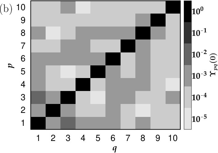 Figure 1
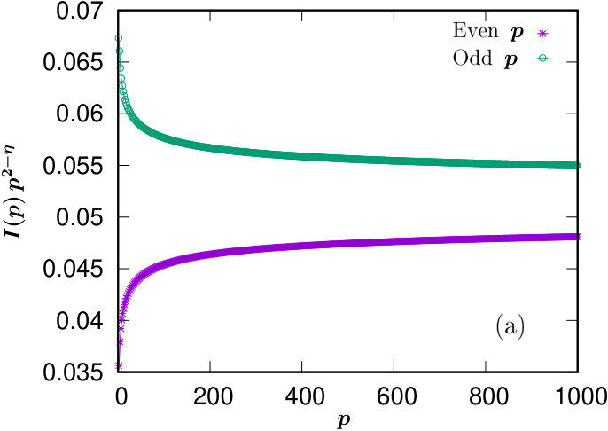 Figure 2
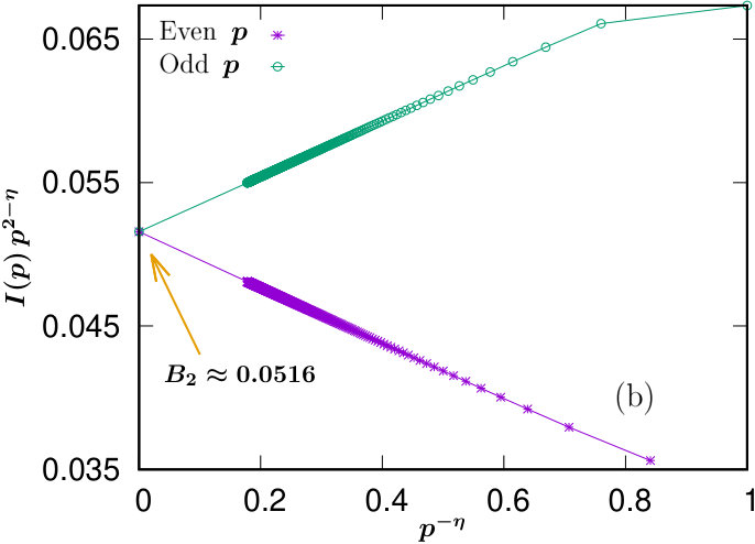 Figure 3
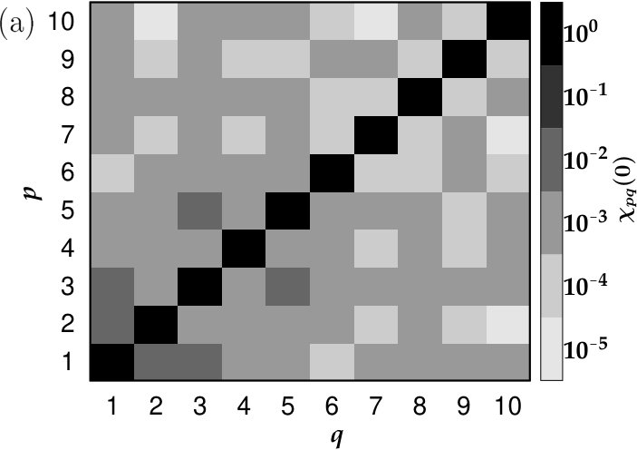 Figure 4
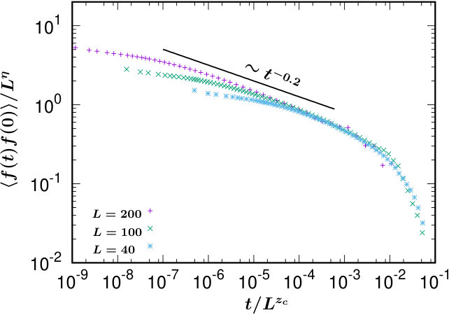 Figure 5
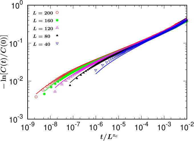 Figure 6
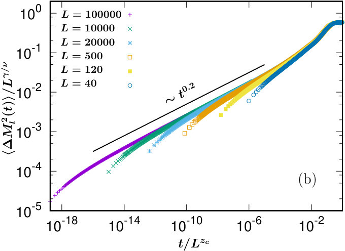 Figure 7
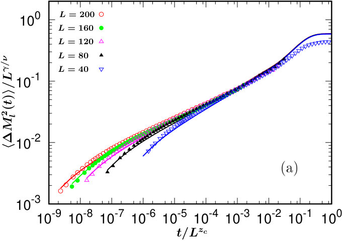 Figure 8
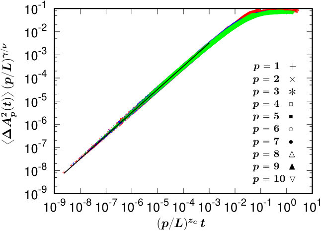 Figure 9
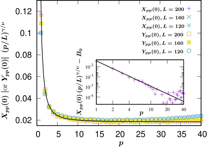 Figure 10
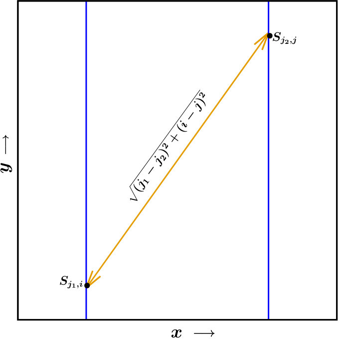 Figure 11
Peer Reviews
No public reviews on file for this paper yet. If you reviewed it on a platform where reviews are public (OpenReview, ICLR, NeurIPS, ICML), you can paste yours below so the community can read it here.
Videos
No videos yet. Explain this paper in a talk, walkthrough, or lecture? Add one.
Approximate dynamical eigenmodes of the Ising model with local
spin-exchange moves
Wei Zhong†
Debabrata Panja†
Gerard T. Barkema†
†Department of Information and Computing Sciences, Utrecht University, Princetonplein 5, 3584 CC Utrecht, The Netherlands
Abstract
We establish that the Fourier modes of the magnetisation serve as the dynamical eigenmodes for the two-dimensional Ising model at the critical temperature with local spin-exchange moves, i.e., Kawasaki dynamics. We obtain the dynamical scaling properties for these modes, and use them to calculate the time evolution of two dynamical quantities for the system, namely the autocorrelation function and the mean-square deviation of the line magnetisations. At intermediate times , where is the dynamical critical exponent of the model, we find that the line magnetisation undergoes anomalous diffusion. Following our recent work on anomalous diffusion in spin models, we demonstrate that the Generalized Langevin Equation (GLE) with a memory kernel consistently describes the anomalous diffusion, verifying the corresponding fluctuation-dissipation theorem with the calculation of the force autocorrelation function.
pacs:
05.10.Gg, 05.10.Ln, 05.40.-a, 05.50.+q, 05.70.Jk
I Introduction
For physical systems in statistical physics, the eigenvalues and eigenvectors (of the Hamiltonians) play a central role. The eigenvectors form a complete orthogonal basis in the space of variables used to express the Hamiltonian. The eigenvalues and eigenfunctions identify the ground and the excited states, as well as their energies, which then form the groundwork for obtaining the partition function, the principal quantity of interest for calculating all equilibrium ensemble-averaged observables.
For classical systems, the Hamiltonian also dictates the dynamics of systems through the equations of motion. Here too, theoretically, the same concept holds, viz. with the equation of motion of a degree of freedom used to describe a Hamiltonian being given by
[TABLE]
with being the friction coefficient in the overdamped limit, it really is an asset to know the dynamical eigenvalues and eigenvectors. Together, the dynamical eigenvalues and eigenvectors ensure that the full time-dependence of any dynamical quantity can be calculated exactly.
In contrast to eigenvalues and eigenvectors of the Hamiltonian itself, the scope for dynamical eigenvalues and eigenvectors is far more restricted, for the following reason. The eigenvectors are linear combinations of all the degrees of freedom , reducing Eq. (1) to the form
[TABLE]
with being the corresponding dynamical eigenvalue, obtained from the diagonalisation of the Hessian matrix . The dynamical eigenmodes , if they exist, are often simply called the modes of the system. For the form (2) to hold, the Hessian must be independent of , which restricts the class of such Hamiltonians only to harmonic ones (i.e., is quadratic in ). Classic examples of such systems are the bead-spring models of linear polymeric systems doi1 ; doi2 , their extensions to star and tadpole polymers rick1 , polymeric membranes nelson ; rick2 , 2D cytoskeleton of cells lipo ; picart ; sack and graphite oxide sheets sack ; hwa ; spec ; wen .
Not all is however lost if the Hamiltonian is not harmonic (which is in fact almost always the case). Note here that any complete orthogonal basis in the space of the degrees of freedom can be used to describe the dynamics of the system. The main disadvantage of choosing an arbitrary one is that the corresponding amplitudes remain dynamically (nonlinearly) coupled at all times, preventing one from taking large time-steps in computer simulations. Despite this shortcoming, sometimes one can be lucky to realise that there are approximate modes that can allow one to take somewhat large time-steps within a preordained error margin. Examples are the Rouse modes for self-avoiding polymers panja1 , a reptating polymer chain panja2 , and polymer chains in a melt kalathi1 ; kreer ; kalathi2 .
The focus of the present paper are the (approximate dynamical) modes of the two-dimensional (2D) square-lattice Ising model (system size ) with local spin exchange moves — commonly known as Kawasaki moves kawasaki — at critical temperature and at zero order parameter, introduced in Sec. II.1. We focus on the line magnetisation for this model and find, surprisingly, that the Fourier modes provide a very good approximation of the true dynamical eigenmodes. We numerically investigate the properties of these modes in Sec. II.2-II.4, numerically revealing that the equilibrium amplitude of the -th mode behaves as , and that its decay time scales , where , and are the three equilibrium critical exponents of the Ising model, and is the critical dynamical exponent for the model with local spin exchange moves halp ; yala ; alex . In Sec. III we use these results to analytically calculate two observables: the autocorrelation function, and the mean-square deviation (MSD), of the line magnetisation. We find that line magnetisation exhibits anomalous diffusion. Our results for anomalous diffusion is consistent with a pattern that the dynamics of magnetisation at the critical temperature in spin models is anomalous walter ; zhong1 ; zhong2 . Importantly, the anomalous diffusion is described by the Generalised Langevin Equation (GLE) zhong1 ; zhong2 (and bears strong resemblance to anomalous diffusion in polymeric and membrane systems under a variety of circumstances rick1 ; rick2 ; panja1 ; panja1a ; panja1b ; panja2b ; maes ; kroy ; popova ; mizuochi ; panja3a ; panja3b ; panja3c ; dubbel ; panja4 ; panja5 ; sakaue ), which we verify in Sec. IV. We conclude the paper in Sec. V.
II The model and the Fourier modes as the approximate dynamical modes
II.1 Ising model with local spin-exchange (Kawasaki) dynamics
We consider the two-dimensional (2D) Ising model on an square lattice with periodic boundary conditions in both - and -directions. The Hamiltonian for the model is given by
[TABLE]
where is the spin value at -location and -location , and is the coupling constant for interactions among the spins and we set during our simulations. The summation runs over all the nearest-neighbour spins, and . All properties we report here have been obtained by simulating the model at the critical temperature , and by setting the value of the Boltzmann constant to unity.
The model is simulated with Kawasaki dynamics at . All simulations reported in this paper have been performed at zero (conserved) order parameter. In other words, we fix the total magnetisation of the system at zero, and at each Monte Carlo move, two neighbouring spins are randomly selected to exchange their values. The resulting energy change is measured, and the move is accepted with the normal Metropolis probability min. For each unit of time, on average, all the spins are supposed to be selected once.
II.2 Fourier modes for line magnetisation
In this model we define the line magnetisation as ; correspondingly, the -th Fourier mode amplitude of the line magnetisation is given by
[TABLE]
where
[TABLE]
respectively are the real and the imaginary parts of the Fourier transform, with . The inverse Fourier transform is then given by
[TABLE]
II.3 Equilibrium properties of the Fourier mode amplitudes
We express the equilibrium correlations of the Fourier modes as
[TABLE]
where the angular brackets () define an average over equilibrated ensembles.
The cross-correlation terms, and respectively, can be argued to be equal to zero, as follows. Let us consider to illustrate the calculation. First, having expressed it as , then making the simultaneous substitutions and , and finally using due to periodic boundary conditions, we find that the term also equals . Next, we use the fact that is only a function of modulo (due to periodic boundary conditions) as well as only of (due to time reversibility invariance at equilibrium). This implies that , leading to the condition . For this reason we leave both and out of further considerations.
Next, we argue that at least up to . In order to do so, we first express as , where . We then again observe, just like in the above paragraph, that is only a function of modulo . This implies that if is an integer, then upon relabelling the line indices the sum trivially reduces to . If however is not an integer, then, we can still relabel the indices as , with , 1 being the lattice unit. Beyond this point, we can do a Taylor expansion of the cosine terms, implying that the equality must hold up to . This, together with the scaling of in the limit for the 2D Ising model as derived in Appendix A, we attempt to fit to the asymptotic scaling in Fig. 1.
From this fit, we find that , where and are two numerically obtained constants. Note also that
[TABLE]
an obvious result obtained from the symmetry of the mode amplitudes under .
The results of Fig. 1 are supplemented with the data for and for and (specifically, to ) in Fig. 2. The values of the off-diagonal elements of and are not zero (we do not expect them to be zero even after caring for numerical accuracy); however, they are at least two orders of magnitude smaller than the diagonal ones.
Together these results indicate that to a very good approximation the modes remain statistically independent during the system’s evolution by means of Kawasaki dynamics.
II.4 Fourier modes as approximate dynamical eigenmodes of the model
In Fig. 3(a), we obtain a data collapse plot for the mean-square deviation (MSD) of the complex mode amplitude , as a function of for for three different system sizes (from our earlier works on spin systems walter ; zhong1 ; zhong2 we expect that the data collapse would require scaling time with a prefactor ). The solid line in the figure then represents
[TABLE]
Since the MSDs of the mode amplitudes can be expressed in terms of their autocorrelation functions as
[TABLE]
with the approximation , for in a large range shown in Fig. 3, Eqs. (9-10) can be recast in the form
[TABLE]
To conclude, in this section we have demonstrated that to a very good approximation the Fourier modes for the 2D Ising model with Kawasaki dynamics remain statistically uncorrelated at all times, and their autocorrelations decay exponentially in time, from which we conclude that they are approximate dynamical eigenmodes. This means that the properties of the modes amplitude can be used to calculate all dynamical quantities to a very good approximation doi1 ; doi2 ; panja1 ; rick1 . In the following section, we will showcase this to calculate the autocorrelation function and the MSD of line magnetisations.
III Dynamics of two physical observables using the Fourier modes as approximate dynamical eigenmodes
In this section we focus on the dynamics observables of the system. Using the properties of the Fourier modes obtained in the last section, we analytically derive the autocorrelation function and the mean-square deviation of the line magnetization.
III.1 Autocorrelation function of the line magnetisation
The first dynamical observable we are dealing with is the autocorrelation function of the line magnetisation, defined as
[TABLE]
This autocorrelation function can be expressed in terms of the modes by combining Eqs. (6), (8) and (12), yielding
[TABLE]
As shown in Fig. 4, the prediction (13) fits the simulation results quite well.
III.2 Anomalous diffusion of the line magnetisation
Let us now consider the MSD of the line magnetisation
[TABLE]
as another dynamical observable.
Using Eq. (6) and , we have
[TABLE]
Then Eq. (15) can be simplified with the approximation , and as the conserved order parameter (chosen to be zero) of the dynamics, leading us to
[TABLE]
Using the properties of and as obtained in Secs. II.3-II.4, the behavior of the MSD of the line magnetisation can be divided into two time domains.
At long times , , meaning that approaches a constant . At intermediate times ,
[TABLE]
As shown in Fig. 5 (a), the prediction (17) fits the simulation results quite well.
For an analytical expression for the msd, with , the sum (17) can be reduced to the following integral:
[TABLE]
but beyond that it is difficult process it further without making approximations. In particular, in the limit and finite values of , the second term within the curly brackets can be dropped. At the lower limit of , the two terms within the curly brackets are however comparable. Nevertheless, if we do drop this second term altogether, then the integral can be easily performed to show that in the leading order of
[TABLE]
This behaviour of the sum (19) is shown in Fig. 5(b).
IV Generalised Langevin Equation formulation for the anomalous diffusion in the Ising model with Kawasaki dynamics
In Sec. III we have demonstrated that at the intermediate time regime, the line magnetisation in the Ising model with Kawasaki dynamics exhibits anomalous diffusion. In our recent studies on the Ising and model with Glauber dynamics zhong1 ; zhong2 , we have argued that the anomalous diffusion of the magnetization belongs to the GLE class, for which the restoring force plays an important role.
Imagine that we choose a tagged line, and since the thermal spin flips, at its magnetisation changes by a little amount . The surrounding spins will react to this change due to the interactions dictated by the Hamiltonian, and it takes time to spread this reaction. During this time, the value of will also readjust to the persisting values of the surrounding spins, undoing at least a part of . It is the latter that we interpret as the result of “inertia” of the surrounding spins that resists changes in , and the resistance itself acts as the restoring force to the changes in the tagged magnetisation, and finally, leads to anomalous diffusion.
IV.1 Generalized Langevin Equation for the line magnetisation
From how the restoring force works introduced before, it not only indicates that there is a memory effect which is significant during the ‘restoring’ process, but also leads us to the GLE formulation to describe the anomalous diffusion.
In line with our previous works on the Ising and model with Glauber dynamics zhong1 ; zhong2 and in polymeric systems rick1 ; panja1a ; panja1b ; panja2b , the relation of the restoring force and the “velocity” of magnetisation can be expressed as
[TABLE]
Here is the internal force, is the “viscous drag” on , is the memory kernel, and are two noise terms satisfying , and the fluctuation-dissipation theorems (FDTs) are given by and respectively.
Equation (20b) can be inverted to write as
[TABLE]
The noise term similarly satisfies , and the FDT . Then and are related to each other in the Laplace space as .
To combine Eq. (20a) and (20b), we obtain
[TABLE]
or
[TABLE]
where in the Laplace space . With , without any loss of generality, using Eq. (23) the result of the velocity autocorrelation is
[TABLE]
where can be calculated by Laplace inverting the relation .
If the memory term is a power law in time, i.e.,
[TABLE]
Using the results from Ref. panja1b , we have
[TABLE]
By integrating Eq. (26) twice in time, we obtain that
[TABLE]
In summary, there is a power-law memory function which plays a vital part in the GLE formulation. From this we can deduce that the anomalous diffusion found in Eq. (17) is non-Markovian and the anomalous exponent is .
IV.2 Verification of the power-law behavior of
Based on the FDT mentioned under Eq. (20b), we now numerically verify the behavior of .
During simulations, at , we thermalise the system to its equilibrium state. For we select a line and fix its value of the magnetisation by performing non-local spin-exchange dynamics, i.e., we choose two lattice site and , if then we exchange their values, else we keep their values as they are. The energy change is measured and we accept the move with the Metropolis probability . For the rest of the system, we let them evolve with the Kawasaki dynamics.
We then keep taking snapshots of the system at regular intervals. For every snapshot we take, we consider an attempt to flip each spin in turn and find the expected change in which would have occurred if this move had been implemented, totalled over all the spins on the selected line, and the possible change of the line magnetisation is defined as . The quantity is plotted in Fig. 6. The figure is in good agreement with our expectation that ; this result has also been observed for the the 2D Ising model with Glauber dynamics zhong1 .
V Conclusion
In this paper, we have studied the Fourier modes of the two-dimensional Ising model with Kawasaki dynamics at critical temperature and at zero (conserved) order parameter. We have established that the Fourier modes are the dynamical eigenmodes of the system to a very good approximation. Using these modes, we can reconstruct the dynamics of any dynamical variable; we have done so for the autocorrelation function and the mean-square deviation (MSD) of line magnetization.
At the intermediate times, we have found that for , the line magnetisation undergoes anomalous diffusion. We have argued that like other spin models and polymeric systems this anomalous behavior can be described by the GLE formulation with a memory kernel. The corresponding fluctuation-dissipation theorem has been verified by the calculation of the force autocorrelation.
With these results, we have showcased that for Kawasaki dynamics, the Fourier modes, as the approximate dynamical eigenmodes, is a useful tool to analytically derive the dynamical quantities in the Ising system. We however note that if the model is evolved using Glauber dynamics, then we find that decays as a stretched exponential in time (not shown in this paper), which clearly shows that the Fourier modes are not the (approximate) dynamical eigenmodes. We do not understand this at present. It could be explored in the future.
Acknowlegement
We thank R. C. Ball for valuable discussions. W.Z. acknowledges financial support from the China Scholarship Council (CSC).
Appendix: Scaling of with for the 2D Ising model
In this appendix we obtain the scaling behaviour of for the 2D Ising model (note that the calculations presented here do not correspond to the total magnetisation of the sample kept fixed at zero, as is the case for Kawasaki dynamics in this paper).
First we calculate the autocorrelation function of the line magnetisation. We use the classic result that at the critical temperature the spin-spin autocorrelation function decays as , where is the Euclidean distance between the two spins and for the 2D Ising model. With that knowledge, upon summing over and in the -direction (see Fig. A1), we obtain
[TABLE]
We next set , and to write,
[TABLE]
The calculation of follows from Eq. (A2) in a similar manner.
[TABLE]
This time setting , Eq. (A3) reduces to
[TABLE]
For , Eq. (A4) leads to , which is the classic result for the equilibrium scaling for the total sample magnetisation for the 2D Ising model.
For we perform the integration over in Eq. (A4) to obtain
[TABLE]
with
[TABLE]
We then perform numerical integration separately for even and odd -values for Eq. (A6). The results, shown in Fig. A2, demonstrate that in the limit
[TABLE]
although convergence to the asymptotic behaviour is rather slow.
The reference list from the paper itself. Each links out to its DOI / PubMed record.
- 1(1) M. Doi, Introduction to Polymer Physics (Oxford University, Oxford, 1996).
- 2(2) M. Doi and S. F. Edwards, The Theory of Polymer Dynamics (Clarendon Press, Oxford, 1988).
- 3(3) R. Keesman, G. T. Barkema, D. Panja J. Stat. Mech. P 02021 (2013).
- 4(4) D. Nelson, T. Piran, and S. Weinberg, Statistical Mechanics of Membranes and Surfaces (World Scientific Publishing, Singapore, 2004).
- 5(5) R. Keesman, G. T. Barkema and D. Panja, J. Stat. Mech. P 04009 (2013).
- 6(6) R. Lipowsky and E. Sackmann, Structure and Dymanics of Membranes, Handbook of Biological Physics Vol. 1 (Elsevier Science, Amsterdam, 1995).
- 7(7) C. Picart and D. E. Discher, Biophys. J. 77 , 865 (1999).
- 8(8) E. Sackmann, Chem Phys Chem 3 , 237 (2002).