Stochastic Optimal Power Flow in Distribution Grids under Uncertainty from State Estimation
Miguel Picallo, Adolfo Anta, Bart De Schutter

TL;DR
This paper addresses the challenge of maintaining voltage levels in distribution grids with uncertain state estimation by formulating a stochastic optimal power flow problem, proposing a tractable solution, and demonstrating its effectiveness through case studies.
Contribution
It introduces a novel stochastic optimal power flow formulation that accounts for state estimation uncertainty and provides a practical, less conservative solution method for distribution grids.
Findings
The proposed method effectively maintains voltage within limits under uncertainty.
Ignoring estimation uncertainty can cause voltage violations.
The approach outperforms deterministic methods in uncertain conditions.
Abstract
The increasing amount of controllable generation and consumption in distribution grids poses a severe challenge in keeping voltage values within admissible ranges. Existing approaches have considered different optimal power flow formulations to regulate distributed generation and other controllable elements. Nevertheless, distribution grids are characterized by an insufficient number of sensors, and state estimation algorithms are required to monitor the grid status. We consider in this paper the combined problem of optimal power flow under state estimation, where the estimation uncertainty results into stochastic constraints for the voltage magnitude levels instead of deterministic ones. To solve the given problem efficiently and to bypass the lack of load measurements, we use a linear approximation of the power flow equations. Moreover, we derive a transformation of the stochastic…
Click any figure to enlarge with its caption.
 Figure 123
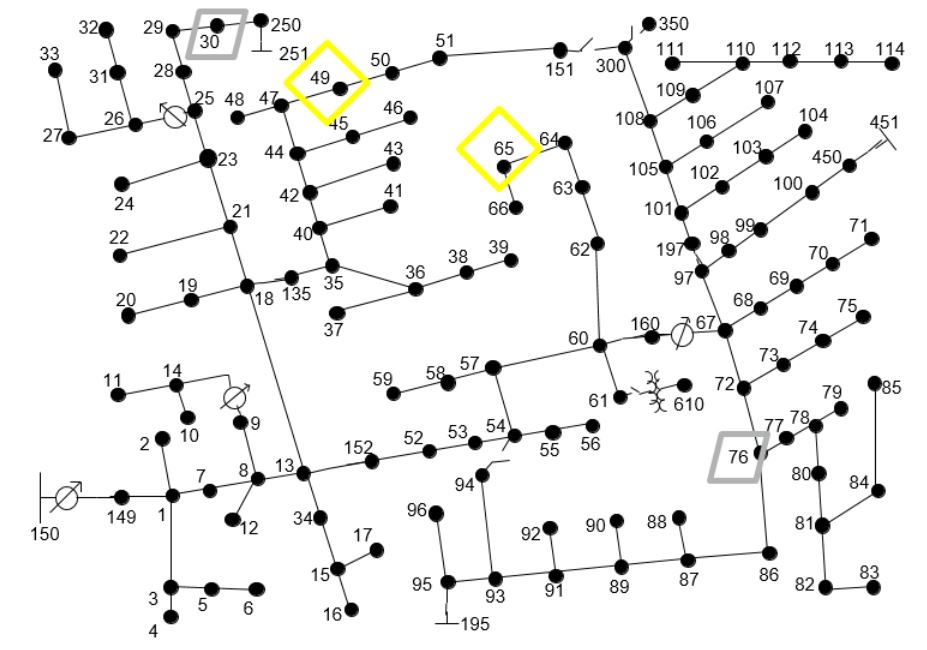 Figure 123
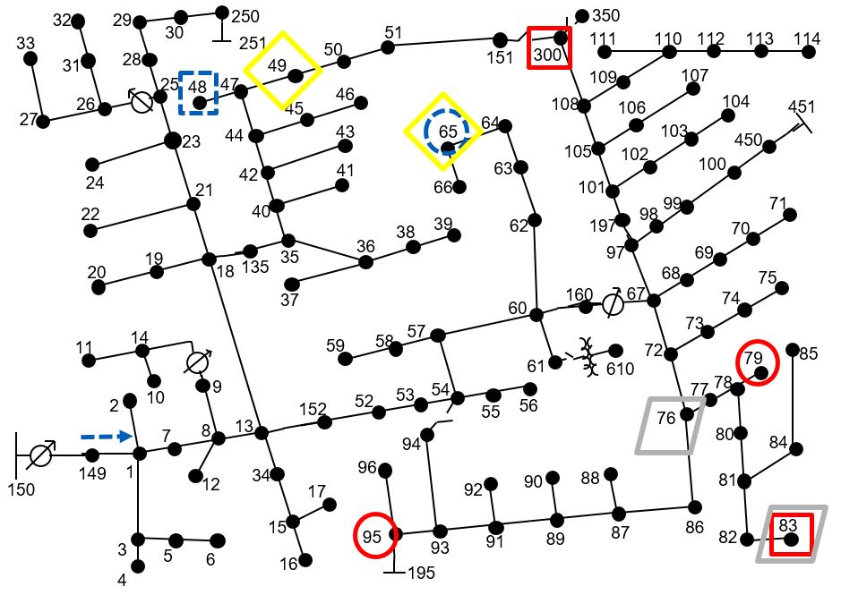 Figure 123
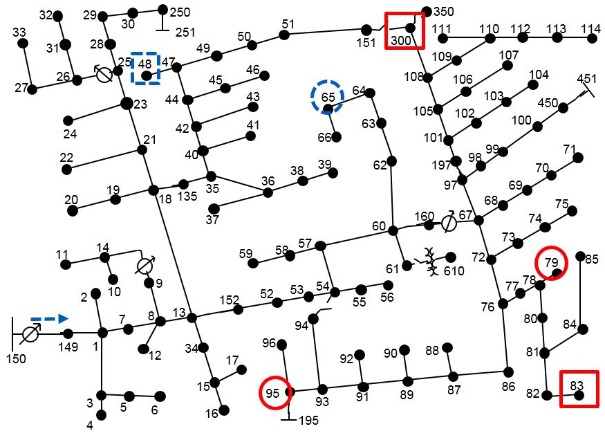 Figure 123
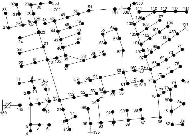 Figure 123
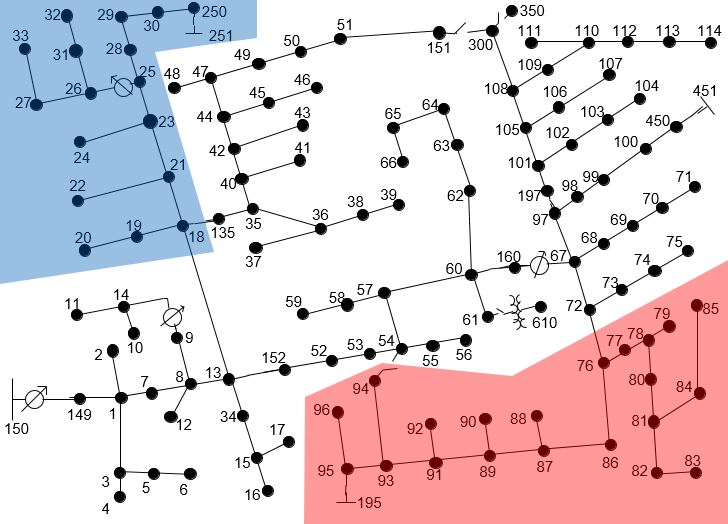 Figure 123
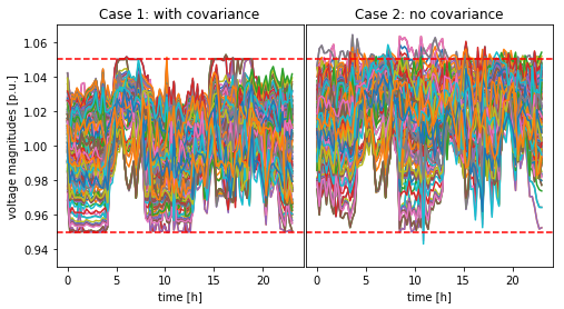 Figure 7
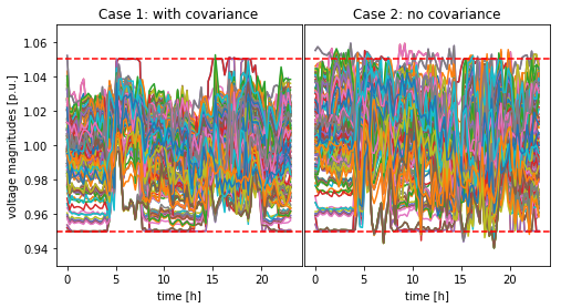 Figure 8
 Figure 9
 Figure 10
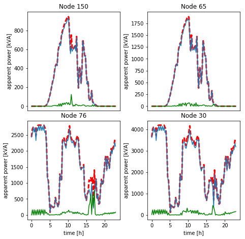 Figure 11
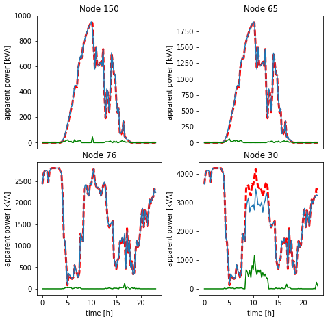 Figure 12
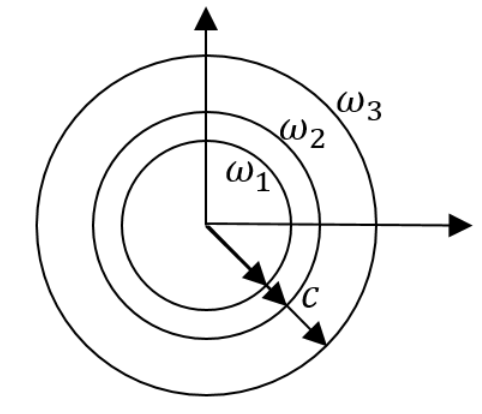 Figure 13
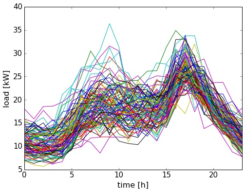 Figure 14
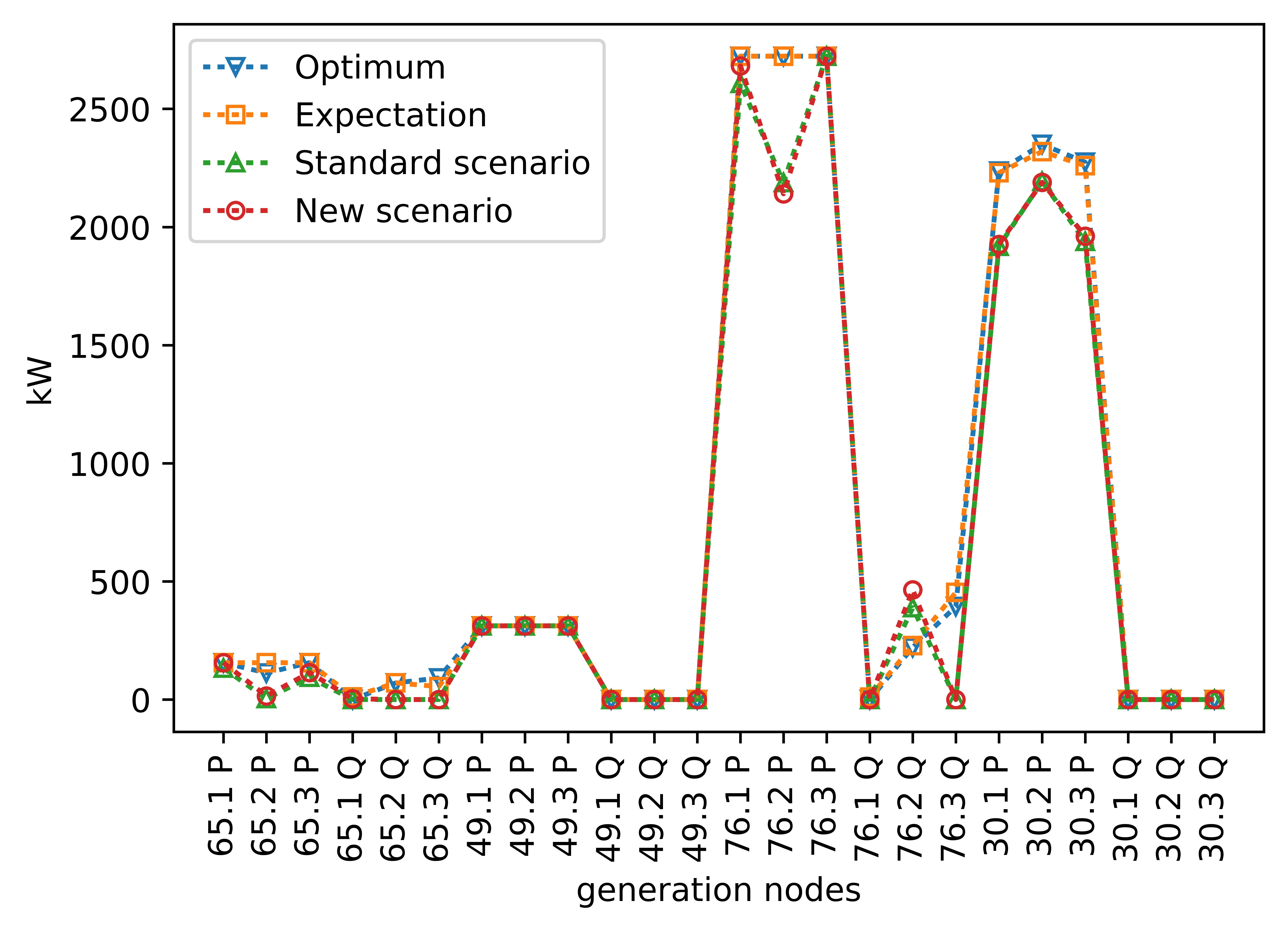 Figure 15
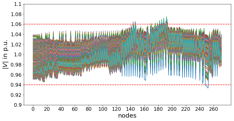 Figure 16
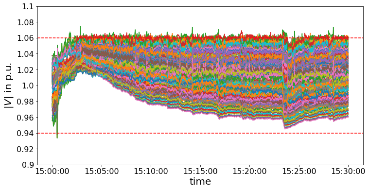 Figure 17
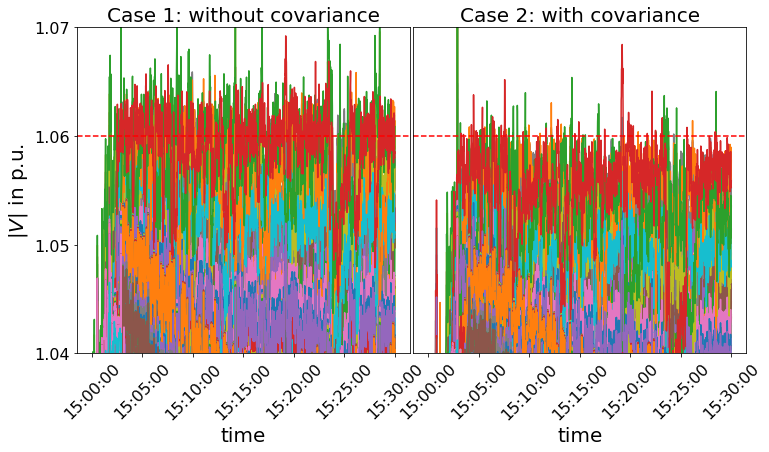 Figure 18
 Figure 19
 Figure 20
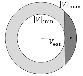 Figure 21
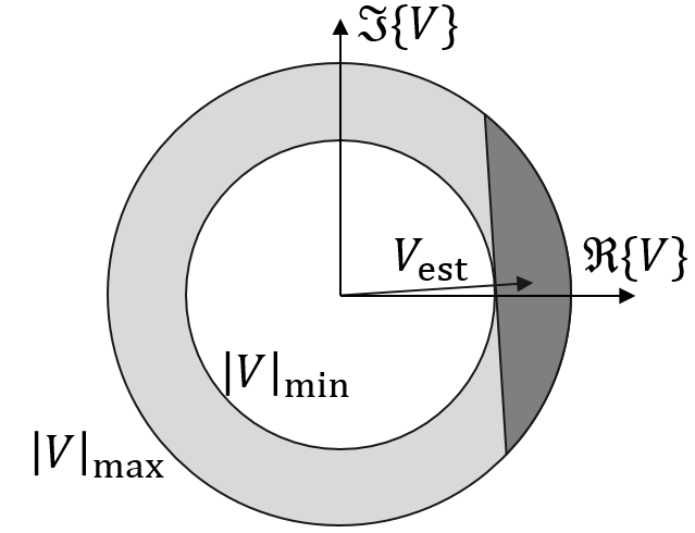 Figure 22
 Figure 23
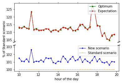 Figure 24
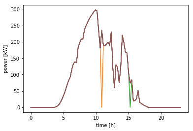 Figure 25
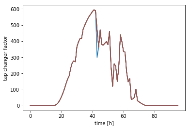 Figure 26
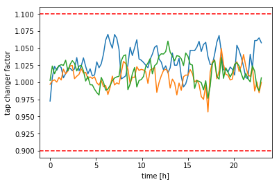 Figure 27
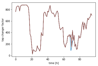 Figure 28
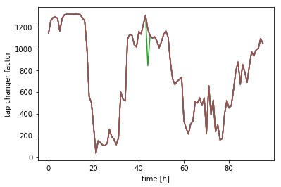 Figure 29
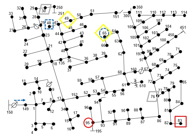 Figure 123
 Figure 123
 Figure 123
 Figure 123
 Figure 123
 Figure 123
 Figure 36
 Figure 37
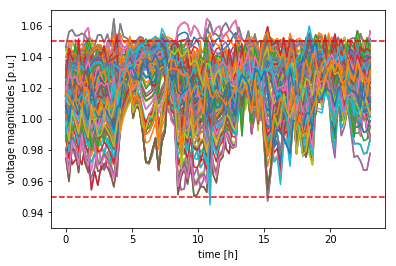 Figure 38
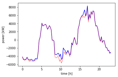 Figure 39
 Figure 40
Peer Reviews
No public reviews on file for this paper yet. If you reviewed it on a platform where reviews are public (OpenReview, ICLR, NeurIPS, ICML), you can paste yours below so the community can read it here.
Videos
No videos yet. Explain this paper in a talk, walkthrough, or lecture? Add one.
Taxonomy
TopicsOptimal Power Flow Distribution · Power System Optimization and Stability · Smart Grid Energy Management
Stochastic Optimal Power Flow in Distribution Grids under Uncertainty from State Estimation
Miguel Picallo, Adolfo Anta and Bart De Schutter This project has received funding from the European Union’s Horizon 2020 research and innovation programme under the Marie Skłłodowska-Curie grant agreement No 675318 (INCITE).M. Picallo and B. De Schutter are with the Center for Systems and Control, Delft University of Technology, The Netherlands {m.picallocruz,b.deschutter}@tudelft.nlA. Anta is with Austrian Institute of Technology [email protected]
Abstract
The increasing amount of controllable generation and consumption in distribution grids poses a severe challenge in keeping voltage values within admissible ranges. Existing approaches have considered different optimal power flow formulations to regulate distributed generation and other controllable elements. Nevertheless, distribution grids are characterized by an insufficient number of sensors, and state estimation algorithms are required to monitor the grid status. We consider in this paper the combined problem of optimal power flow under state estimation, where the estimation uncertainty results into stochastic constraints for the voltage magnitude levels instead of deterministic ones. To solve the given problem efficiently and to bypass the lack of load measurements, we use a linear approximation of the power flow equations. Moreover, we derive a transformation of the stochastic constraints to make them tractable without being too conservative. A case study shows the success of our approach at keeping voltage within limits, and also shows how ignoring the uncertainty in the estimation can lead to voltage level violations.
I Introduction
The increased share of distributed generation and controllable loads presents many advantages for the distribution grid but at the same time requires new techniques and approaches to guarantee a proper operation of the grid. Traditional strategies for distribution grids rely on the so-called fit-and-forget policy, where most design questions are solved during the planning stage [1]. However, profiles for renewable generation and electric vehicles are hard to predict and an offline solution that ignores the actual state of the system would lead to a very inefficient and even dangerous operation of the grid, where operating requirements may be violated. To face these new challenges, optimal power flow (OPF) strategies commonly used for the transmission grid, are being adapted to distribution grids.
However, traditional simplifications in transmission grids like the decoupled fast power flow [2] are not suited for distribution grids, given the presence of coupled phases, unbalanced loads, and lower ratios in these types of grids. The OPF problem is a non-convex NP-hard problem [3]. Some convexification strategies use a linear approximation around a given operating point [4, 5]. Other use a semidefinite programming reformulation [6] in order to avoid a linear approximation, but require a rank relaxation in order to be convex.
Moreover, the solution of the OPF is naturally dependent on the state of the grid (voltages, currents, loads, etc.), which at the distribution level is only partially known. Indeed, while enough sensors are usually available in transmission grids, this is not the case for distribution grids, where state estimation (SE) algorithms [7, 8] rely on load/generation forecasts, grid topology knowledge, and a relatively low number of measurements in order to identify the actual grid status [9, 10]. These SE algorithms provide an estimation of the variables of interest (e.g. grid voltages), with a certain degree of uncertainty. Ignoring this uncertainty in the SE estimates could lead to voltage limit violations. However, many OPF formulations assume that the values of the voltages or loads across the network are available [5, 6]. In [4] only a few measurements are deployed, but then the constraints on the operating limits are required only in the nodes with measurements and not in the rest. Some papers introduce chance constrained optimization methods to account for the uncertainty in the loads and generation, like using convex relaxations [11, 12], or an scenario based approach enabling the possibility to add real-time sensors in [13]. But these methods may be suboptimal and not suited for real-time operation of large systems with many loads, since they may either require introducing a large number of constraints [13], or a considerable amount of sampling as well as computing expectations from many probability distributions in each optimization step [12].
In this work we start considering a standard formulation of an OPF problem, where the controllable elements are a set of distributed generation sources and tap changers in distribution transformers. Instead of load measurements [5, 6], since they may not be available, we consider an estimate from a SE as input to our OPF problem; and thus the voltage variables are described as stochastic signals, which lead to stochastic constraints for the OPF problem. Our approach relies on a linear approximation of the power flow equations around the operating point, which allows to bypass the lack of load measurements. Additionally, we reformulate the stochastic constraints using the probability distribution of the voltages given by the SE algorithm, to make the problem tractable without being too conservative. Our framework is not limited to one particular SE algorithm, but instead we consider a generic unbiased estimate with a Gaussian distribution and a known covariance matrix. Thus, our main contributions are the use of a generic SE algorithm for the OPF problem, to avoid requiring full load measurements; and a transformation of the resulting stochastic constraints produced by the uncertainty in the voltage estimates, to guarantee the voltage limits in all nodes, even those without measurements, as opposed to [4].
The rest of the paper is distributed as follows: Section II defines the grid model, while Section III describes the standard outcome of an SE algorithm, which would be considered as input to our OPF formulation. Section IV formulates the OPF problem including the stochastic constraints, and states the main contribution of this paper. Finally, a 123-bus test feeder is considered in Section V to show the perils of ignoring the uncertainty coming from the estimation step and the effectiveness of the proposed approach to solve this.
II Distribution Grid Model
A distribution grid consists of buses, where power is injected or consumed, and branches, each connecting two buses. This system can be modeled as a graph with nodes representing the buses, edges representing the branches, and edge weights representing the admittance of a branch, which is determined by the length and type of the line cables.
In 3-phase networks buses may have up to 3 phases, so that the voltage at bus , with phases, is (and the edge weights ). The state of the network is then typically represented by the vector bus voltages , where denotes the known voltage at the source bus, and the voltages in the non-source buses, where depends on the number of buses and phases per bus.
Using the Laplacian matrix of the weighted graph , called admittance matrix [7], the power flow equations to compute the currents and the power loads are:
[TABLE]
where is the imaginary unit, the active and reactive loads, denotes the complex conjugate, represents the diagonal operator, converting a vector into a diagonal matrix.
III State Estimation
We consider a standard SE algorithm [7, 8] that provides an unbiased estimation of the network voltages denoted as , in rectangular coordinates, and a covariance matrix representing its uncertainty in rectangular coordinates . This uncertainty is mainly caused by the use of highly uncertain pseudo-measurements, such as load predictions, to compensate for the lack of measurements [9, 10]. The true voltages , , can then be expressed as:
[TABLE]
where represents the identity matrix. These voltages denote the previous voltages before solving the OPF and applying the new control set points.
This uncertainty represented in is especially relevant when considering distribution networks, where only few measurements are available and the SE algorithm needs to rely on noisy load predictions [10]. Given that is not available, only can be used to regulate distributed generation sources and other controllable elements at the distribution level.
Remark 1
For convenience, we have considered the estimation in rectangular variables, but if the SE provides the results in polar variables, the covariance in rectangular coordinates could still be estimated using the Jacobian of the mapping from polar to rectangular coordinates.
IV Optimal Power Flow
The OPF problem seeks to regulate the controllable elements in the network in order to optimize its operation under some safety conditions. This optimization typically focuses on minimizing costs, energy loses, etc.; the controllable elements are distributed energy sources, tap changers, batteries, flexible loads, network configuration, etc.; and the safety conditions are typically voltage and current limits on buses and connections.
In this paper, we consider as controllable elements the distributed generation sources at the distribution level , where denotes the set of nodes with distributed renewable energy sources; and the set points of the voltage tap changers for every phase in the transformers . For simplicity, the objective is to minimize the total amount of energy required from the substation , and thus to minimize the cost of external energy required and to prioritize the renewable energy generated within the network. Other similar OPF formulations, with e.g. other possible objectives, can be addressed with our solution, mutatis mutandis. The safety conditions are given by the limits for the voltage magnitudes . Moreover, the power flow equations in (1) represent another algebraic constraint for the OPF problem. In this work we do not consider dynamic elements like batteries; so we can solve the following OPF problem at every instance:
Definition 1
Standard OPF:
[TABLE]
where denote the voltage magnitude limits, denote the available energy limits at node , and denotes the admittance matrix as a function of the vector of voltage tap changers . The variables to optimize are then the power supplied by the substation and the renewable energy sources , , the voltage tap changers , and the voltages and . Among the variables, the control elements are , and , while and are determined by the constraints. The loads at the rest of the nodes are inputs to the OPF problem, and are typically measured or estimated.
There are some problems with the OPF in (3):
- •
The power flow equation in (3l) is nonlinear and thus difficult to handle.
- •
The problem is not convex due to (3l), and also due to the lower limit in (3w) if considering rectangular coordinates. However, we would like to have a convex problem in order to guarantee optimality.
- •
In (3l), both the loads in the nodes other than the substation and the renewable sources: , where denotes the set of nodes in the source bus, and the voltages in the nodes other than the source nodes are not known, since we assume that we have a distribution network with few sensors and only a voltage estimate is provided by the SE. So only plus some other measurements are known.
- •
Since there is a degree of uncertainty in the SE estimates represented in the covariance matrix , we need to take it into account for the voltage limits in (3w).
- •
The discrete variable in (3o) converts the given problem into an integer problem.
Remark 2
For simplicity, we are not considering in (3) the thermal constraints limiting the amount of current through the lines: , where would be the line admittance matrix mapping voltages to line currents, and the vector of maximum values allowed. Nonetheless, these constraints define a convex region on , and therefore could be easily included.
IV-A Transformer Approximation
In order to include the tap changers more efficiently and to simplify in (3l), we assume electrical isolation at the transformers and thus consider different subsystems related by the tap changers equations similar to [14]. For simplification, we consider a system with only one controllable transformer with tap changers, and we assume that the ordering of nodes in (1), in and , is already such that the nodes of the first subsystem appear first, and then those of the second, with the nodes connected to the transformer appearing one after the other, so that we have:
[TABLE]
where represent the voltages of each subsystem except the nodes of the transformer, correspond to the nodes of the transformer for each subsystem, is the admittance with isolated subsystems, represent the admittance matrix of each subsystem, and is the admittance matrix of the transformer. Then the power flow equations can be expressed as:
[TABLE]
We have disregarded the admittance of the transformer in (4), assuming that it is large enough and that the voltage drop can be neglected. If needed, it could be included using an artificial node as in [14]. To further simplify (3o), we will also consider a continuous tap changer for every phase , instead of . Its values could afterwards be rounded to the closest discrete value as proposed in [14].
Remark 3
This transformer approximation could easily be extended to a system with more controllable transformers by splitting the system in more subsystems.
IV-B Power Flow Approximation
Instead of considering the power flow equations in (3l) directly, we consider a first-order linear approximation similar to the one in [4] around the estimated voltage states and the known voltages at the source nodes , both prior to the optimization step:
[TABLE]
where represent the deviations of values after the optimization process; denote the values before applying the new set points produced by the optimization step; and are the values after the optimization step, so we have:
[TABLE]
With this approximation we have a second-order error of the type and , which we consider negligible since deviations are expected to be small, because they will be constrained by the voltage magnitude constraints (3w). Note that (6) is not linear in the decision variables due to the complex conjugates . Note that the equation is sufficient to imply in (6), since is already satisfied by .
Remark 4
We consider that the optimization process is fast enough, so that the loads remain constant. Therefore we have for , where denote the set of nodes on the primary and secondary sides of the transformer respectively, and we do not need to measure or estimate the values of the loads. This is very relevant, since it allows to bypass the lack of load measurements. To achieve this fast optimization process, we can use an early stopping optimization or the recent work on projected gradient online optimization methods for the OPF problem in [4, 5]. Moreover, this fast optimization allows to avoid outdated setpoints and thus suboptimal solutions as remarked in [4].
Furthermore, if we consider a rectangular representation of the variables we can express (6) linearly on the decision variables, and the real and imaginary parts of :
[TABLE]
where depends only on and , both known, and can be expressed as:
[TABLE]
with
[TABLE]
IV-C Stochastic Voltage Limits
Since we only have an estimation of the voltage previous to the optimization step (2), the voltage after the optimization step , , will be a prediction with a covariance:
[TABLE]
Since is then unknown, we cannot set a deterministic voltage limit constraint like (3w). Therefore, we use a stochastic one instead:
[TABLE]
where is a desired threshold probability level, like , which can be tuned to increase the confidence level of the constraint. This constraint converts the OPF problem into a chance constrained optimization problem. We use the following theorem to reformulate (9) as a function of our decision variables , our estimation , and in (2). We use and to denote the blocks corresponding to the covariance of the real and imaginary parts respectively.
Theorem 1
For all , there exists such that if the following constraints holds for all :
[TABLE]
then (9) is satisfied. We use to denote all possible combinations to represent all constraints.
Furthermore, can be found using standard tables for Gaussian distributions by choosing such that
[TABLE]
Proof:
We first split the constraint in (9) into two independent conditions for and :
[TABLE]
so that
[TABLE]
where for simplicity we have divided by , but other options would also be possible. In rectangular coordinates, inequalities inside the probability in (12) describe an annulus, which clearly is a non-convex region. Since we want to convert (3w) into a convex constraint, we consider the biggest convex region around the operating point and included in the annulus (see Fig. 1):
[TABLE]
Then the lower bound in (12) is replaced by the inequality representing the dark grey area in Fig. 1:
[TABLE]
Considering the estimation covariance in rectangular coordinates , using (8) we can expand as a function of the voltage deviations of our power flow formulation (7):
[TABLE]
where , with , denote the noises of the real and imaginary parts of the voltage estimation at node : , see (2). Using the diagonal decomposition , we can rewrite these noises as different linear combinations of the same noise vector:
[TABLE]
Provided that conditions (10) are satisfied, we can use the voltage expressions (15) to express (12) as a function of the noises :
[TABLE]
and
[TABLE]
We can now use the distributions of and in (16) to derive the way to choose in (11) to satisfy (12). For a given threshold , since and are not independent, we can formulate the following inequality:
[TABLE]
Using the Gaussian distribution tables to choose such that
[TABLE]
then we have
[TABLE]
Using (17) and (18) we finally obtain:
[TABLE]
so that (12) and (14) are satisfied and so is (9). ∎
Remark 5
The convex approximation in (14) may cause a loss of optimality in the OPF problem. However, it helps to avoid that the phase angle of the voltages deviates too much from the base voltages, which is also not desirable.
The advantage of using our approach to deal with the chance constraints (9) is that we separate the SE process from the OPF problem. Real-time sensors can be efficiently managed by the SE process [10], and during the real-time operation of the network, we avoid sampling and/or computing convex approximations of the chance constraints using the conditional value at risk as in [12].
IV-D Final OPF
Using Thm. 1 we can rewrite (9) into a convex deterministic constraint, so that it can be integrated into our OPF problem:
Definition 2
OPF with linear power flow approximation and stochastic voltage limits:
[TABLE]
where now the variables to control are , and , while , and are determined by the constraints. All previous values before the optimization step, , are stored from the control step before the current one, and and are given by the SE.
Remark 6
Note that the OPF problem in (23) is convex, and thus can be solved optimally and efficiently using state-of-the-art convex-optimization algorithms [15].
V Case Study
A simulation of 24 hours with 15 min intervals is run on a test case to test the effectiveness of the methodology. Here we describe the settings of the test case and analyze the results. The algorithms are coded in Python and run on an Intel Core i7-5600U CPU at 2.60GHz with 16GB of RAM.
V-A Settings
- •
System: We use the 123-bus test feeder available online [16, 17], see Fig. 2.
- •
Measurements for the SE (see Fig. 2): As in [10], voltage measurements (red circle for phasor, red square for magnitude only) are placed at buses and , current measurements (blue dashed circle for phasor, blue dashed square for magnitude only) at buses and , and branch current phasor measurements (blue dashed arrow) at branch (after the regulator) .
- •
Load Profiles: As in [10] for the SE, the load profiles are built by aggregating a several households profiles.
- •
Distributed Generation: Solar energy is introduced in the three phases of nodes and , and wind energy in nodes and , see Fig 2 (a yellow rhombus for solar, a grey parallelogram for wind). The profiles can be seen in Fig. 5. They are simulated using a solar irradiation profile and a wind speed profile from [18, 19]. We use these profiles to determine for each time step the apparent power limit for in (23ag).
- •
Tap changers: We control the transformer located in the branch , see Fig. 2, and set the tap changers limits at , as in [14].
- •
Voltage limits: The common values and are used for the voltage magnitude constraints [14, 4].
- •
Other values: The probability limit for the stochastic constraints (9) is chosen to be the standard value , resulting in .
V-B Results
To prove the effectiveness of our approach, we compare the resulting voltage magnitudes when controlling the transformer and the introduced energy in two cases: in case 1, we take the uncertainty into account, using the covariance to ensure the voltage limit constraints; while in case 2, we are using the voltage estimates as if they were the true values, without taking into account the covariance. It can be observed in Fig. 3 that case 1, using the covariance, performs much better than case 2 in controlling the voltage magnitudes within their limits.
From the case 1 using the covariance, we can also observe in Fig. 4 how the tap changers remain within the limits, and their value changes to optimize the operation of the grid. Furthermore, we can also observe in Fig. 5 how the whole energy available is not always fully used. This happens because otherwise some voltage constraints would be violated. Precisely, in Fig. 3 it can be observed that the instants at which some of the available energy is not used, coincide with some voltage magnitudes being at the limit.
Moreover, note that the load profiles introduced in the SE are not necessarily normally distributed, and thus the SE estimate may have a non-Gaussian probability distribution. However, our approach in case 2 still succeeds in keeping the voltages within limits.
VI Conclusions
In this work, we have presented a methodology to combine the state estimation (SE) with the optimal power flow (OPF) problem for a distribution grid where only a few measurements are available. The lack of sensors produces uncertain voltage state estimates, and therefore we have adapted the standard OPF to include stochastic constraints for the voltage magnitude levels. Moreover, we use a linear approximation of the power flow to convexify the problem and bypass the lack of load measurements using delta increments. We also transform the stochastic constraints to make them tractable for our problem, by using the probability distribution of the state estimation. Finally, we prove through a case study, that the proposed methodology succeeds in controlling a large distribution grid with some controllable elements, like transformers and distributed generation, while respecting the voltage constraints.
Future work could include adding controllable elements with dynamics, like batteries, or flexible loads, like electrical vehicles. Additionally, we could also consider the discrete nature of the tap changer values in the transformer, as well as other probability distributions for the voltage SE.
The reference list from the paper itself. Each links out to its DOI / PubMed record.
- 1[1] J. B. Ekanayake, N. Jenkins, K. Liyanage, J. Wu, and A. Yokoyama, Smart grid: technology and applications . John Wiley & Sons, 2012.
- 2[2] B. Stott and O. Alsaç, “Fast decoupled load flow,” IEEE Transactions on Power Apparatus and Systems , no. 3, pp. 859–869, 1974.
- 3[3] J. Lavaei and S. H. Low, “Zero duality gap in optimal power flow problem,” IEEE Transactions on Power Systems , vol. 27, pp. 92–107, Feb 2012.
- 4[4] E. Dall’Anese and A. Simonetto, “Optimal power flow pursuit,” IEEE Transactions on Smart Grid , vol. 9, pp. 942–952, March 2018.
- 5[5] A. Hauswirth, S. Bolognani, G. Hug, and F. Dörfler, “Projected gradient descent on riemannian manifolds with applications to online power system optimization,” in 54th Annual Allerton Conference on Communication, Control, and Computing (Allerton) , pp. 225–232, Sept 2016.
- 6[6] E. Dall’Anese, H. Zhu, and G. B. Giannakis, “Distributed optimal power flow for smart microgrids,” IEEE Transactions on Smart Grid , vol. 4, pp. 1464–1475, Sept 2013.
- 7[7] A. Abur and A. G. Exposito, Power System State Estimation: Theory and Implementation . CRC Press, 2004.
- 8[8] A. Monticelli, “Electric power system state estimation,” Proceedings of the IEEE , vol. 88, no. 2, pp. 262–282, 2000.