Sharp bounds on the relative treatment effect for ordinal outcomes
Jiannan Lu, Yunshu Zhang, Peng Ding

TL;DR
This paper derives sharp bounds for the relative treatment effect in ordinal outcomes, allowing for arbitrary dependence between potential outcomes, which enhances interpretability when the average treatment effect is ill-defined.
Contribution
It provides the first derivation of sharp bounds on the relative treatment effect for ordinal outcomes without assuming independence of potential outcomes.
Findings
Derived sharp bounds on the relative treatment effect for ordinal outcomes.
Bounds are identifiable from observed data and accommodate arbitrary dependence.
Enhances interpretability of treatment effects in ordinal outcome studies.
Abstract
For ordinal outcomes, the average treatment effect is often ill-defined and hard to interpret. Echoing Agresti and Kateri (2017), we argue that the relative treatment effect can be a useful measure especially for ordinal outcomes, which is defined as , with and being the potential outcomes of unit under treatment and control, respectively. Given the marginal distributions of the potential outcomes, we derive the sharp bounds on which are identifiable parameters based on the observed data. Agresti and Kateri (2017) focused on modeling strategies under the assumption of independent potential outcomes, but we allow for arbitrary dependence.
Click any figure to enlarge with its caption.
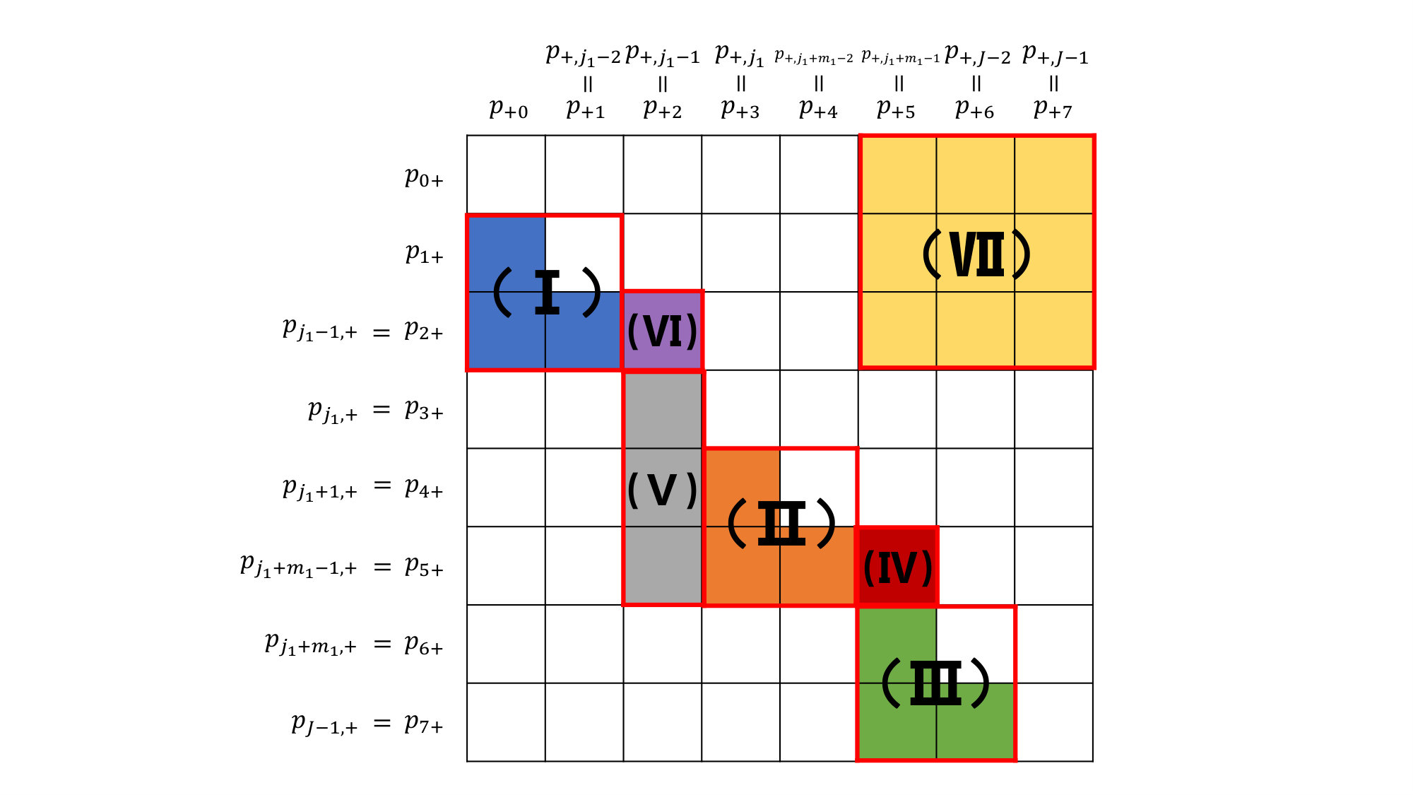 Figure 1
Peer Reviews
No public reviews on file for this paper yet. If you reviewed it on a platform where reviews are public (OpenReview, ICLR, NeurIPS, ICML), you can paste yours below so the community can read it here.
Videos
No videos yet. Explain this paper in a talk, walkthrough, or lecture? Add one.
Taxonomy
TopicsHealth Systems, Economic Evaluations, Quality of Life · Advanced Causal Inference Techniques · Statistical Methods and Inference
Sharp bounds on the relative treatment effect for ordinal outcomes
Jiannan Lu
Yunshu Zhang and Peng Ding Jiannan Lu is Senior Data Scientist (E-mail: [email protected]), Analysis and Experimentation, Microsoft Corporation, Redmond, WA 98052, U.S.A. Yunshu Zhang is Doctoral Student (E-mail: [email protected]), Department of Statistics, North Carolina State University, Raleigh, NC 27695, U.S.A. Peng Ding is Assistant Professor (E-mail: [email protected]), Department of Statistics, University California, Berkeley, CA 94270, U.S.A.
Abstract
For ordinal outcomes, the average treatment effect is often ill-defined and hard to interpret. Echoing Agresti and Kateri, (2017), we argue that the relative treatment effect can be a useful measure especially for ordinal outcomes, which is defined as , with and being the potential outcomes of unit under treatment and control, respectively. Given the marginal distributions of the potential outcomes, we derive the sharp bounds on which are identifiable parameters based on the observed data. Agresti and Kateri, (2017) focused on modeling strategies under the assumption of independent potential outcomes, but we allow for arbitrary dependence.
Keywords: Causal inference; partial identification; potential outcomes
Causal inference with ordinal outcomes
Ordinal outcomes are very common in empirical research (e.g., Whitehead et al., 2001; Scharfstein et al., 2004; Huang et al., 2017; Liu and Zhang, 2018). Consider a binary treatment and an ordinal outcome with labels , where 0 and denote the worst and best categories, respectively. Define as the potential outcomes of unit under treatment and control, respectively. For all let denote the probability that the potential outcome is under treatment and under control, respectively. The probability matrix characterizes the joint distribution of the potential outcomes. Let and be the marginal distributions of the potential outcomes under treatment and control, respectively. We let and denote the marginal probability vectors.
For ordinal outcomes, the average treatment effect is often hard to interpret, if there is no clear definition of “distance” between different categories. In contrast, the parameters and have clear interpretations as the probabilities that the treatment is beneficial and strictly beneficial for the outcome (Newcombe, 2006b ; Newcombe, 2006a ; Zhou, 2008; Huang et al., 2017; Lu et al., 2018). Recently, Agresti and Kateri, (2017) used the relative treatment effect for ordinal outcomes (Agresti, 2010), defined as
[TABLE]
We can verify that The parameters , and are closely related to the classic Wilcoxon–Mann–Whitney statistic for testing equality of two distributions (Kruskal, 1952, 1957; Klotz, 1966; Vargha and Delaney, 1998; Chung and Romano, 2016; Divine et al., 2018). The parameters , and depend on the joint distribution of the potential outcomes and are not identifiable based on the observed data (Hand, 1992; Demidenko, 2016; Huang et al., 2017; Lu et al., 2018; Greenland et al., 2019). Huang et al., (2017) obtained numerical bounds on and , and Lu et al., (2018) derived explicit formulas of these bounds. Agresti and Kateri, (2017) and Cheng, (2009) discussed assuming independent potential outcomes implicitly and explicitly. Chiba, (2018) proposed a Bayesian approach to infer , which requires imposing a prior on the joint distribution of the potential outcomes. Fay et al., (2018) and Fay and Malinovsky, (2018) pointed out the non-identifiability nature of and proposed a non-sharp bound on given the marginal distributions of and based on Lu et al., (2018)’s bounds on and
For (i.e., when is binary), the relative treatment effect reduces to which is actually the average treatment effect. Because the average treatment effect depends only on the marginal distributions of the potential outcomes, is identifiable from the observed data with . However, becomes unidentifiable when , because it depends on the joint distribution of the treated and control potential outcomes. We adopt the partial identification strategy (c.f. Manski, 2003; Richardson et al., 2014) and focus on the sharp bounds on . We compute the maximum and minimum values of that are compatible with the marginal distributions of the potential outcomes. As a theoretical starting point, we assume that the marginal probabilities and are known, and later we will incorporate sampling variability. The sharp upper bound is the solution of the following linear programming problem:
[TABLE]
The sharp lower bound is the corresponding minimum value subject to the same set of constraints. By definitions, the sharp upper and lower bounds are functions of the marginal probabilities and , although the relative treatment effect itself is a function of the joint probability matrix Balke and Pearl, (1997) and Huang et al., (2017) used linear programming to obtain bounds on different causal parameters for ordinal and more general outcomes. Numerically, we can easily obtain the values of and for given values of and . However, our goal here is to derive explicit formulas, as in Balke and Pearl, (1997) and Lu et al., (2018), which give more transparent interpretations and allow for convenient estimation and inference.
The rest of the paper is organized as follows. Section 2 derives the sharp bounds on the relative treatment effect. Section 3 discusses the statistical inference based on the derived bounds under different scenarios such as completely randomized experiments and observational studies. Section 4 presents two examples to illustrate our proposed method. We relegate all technical details to the supplementary material.
Main results: Sharp bounds on
2.1 Notation
We introduce a few quantities that are needed to express the sharp bounds on . For each fixed and let
[TABLE]
Define the summation to be zero when the range is empty, e.g., if Importantly, the ’s depend only on the marginal probabilities and Before moving forward, we provide insights on the important roles the ’s play in deriving the sharp bounds on the relative treatment effect For example, by taking the difference between
[TABLE]
and
[TABLE]
we obtain
[TABLE]
In other words, is a loose upper bound on Similarly, we can prove that other ’s are also loose upper bounds on Interestingly, in the next subsection we will show that the ’s together can sharply bound .
2.2 Main theorem, corollaries and remarks
We now present the main result of this paper.
Theorem 1**.**
When , the sharp upper bound on the relative treatment effect is
[TABLE]
In the supplementary material we provide a proof of Theorem 1, which consists of two parts. First, as previously mentioned, we show that for and Second, we prove the sharpness of by directly constructing a probability matrix attaining the bound given the marginal distributions. Although not affecting the proof, it is worth noting that the probability matrix attaining might not be unique in general.
By switching the labels of the treatment and control potential outcomes, it is straightforward to obtain the sharp lower bound on the relative treatment effect
Corollary 1**.**
When , the sharp lower bound on the relative treatment effect is
[TABLE]
where for all and
[TABLE]
with summations being zero if the range is empty.
Remark 1**.**
For , we can verify that and and that and Consequently, the sharp lower bound in Theorem 1 reduces to and the sharp upper bound in Corollary 1 reduces to
Intuitively, and correspond to “extremely” positive and negative associations between potential outcomes and In practice, because they are characteristics of the same unit, it is plausible to rule out the scenarios with negatively associated potential outcomes (Ding and Dasgupta, 2016; Lu et al., 2018). Therefore, we can use the previous result with independent potential outcomes as a lower bound (Cheng, 2009; Agresti, 2010; Agresti and Kateri, 2017).
Corollary 2**.**
With independent potential outcomes, i.e., , the relative treatment effect can be identified as
We suggest using as the bounds on as in the examples in Section 4.
Statistical modeling and inference
3.1 Point estimation
To estimate the sharp bounds of the relative treatment effect we first estimate the marginal probabilities of the potential outcomes. Let be the binary treatment indicator, with if unit receives treatment and if unit receives control. The observed outcome is therefore . In some studies, we also have pretreatment covariates . We assume that the observations are independent and identically draws from a super population. Following Lu et al., (2018), we consider the following two scenarios:
Completely randomized experiment with . Therefore, we can estimate the marginal probabilities by their sample analogues
[TABLE] 2. 2.
Unconfounded observational study with . For illustration, we focus on the propensity score weighting and outcome modeling approaches. First, we can estimate the marginal probabilities by the inverse propensity score weighting:
[TABLE]
where is the fitted value of the propensity score , for example, via a logistic regression of the treatment indicator on the covariates. Second, we can fit two outcome models and using the data under treatment and control, respectively. A canonical choice for ordinal outcomes is the proportional odds model (c.f. Agresti, 2010). We then obtain the fitted values and for all units. The final outcome-regression estimators for the marginal probabilities are and We can estimate the bounds using a plug-in approach after obtaining the ’s and ’s.
3.2 Sharpening bounds using covariates
Agresti and Kateri, (2017)’s strategy of covariate adjustment is slightly different from the above discussion in Section 3.1. Agresti and Kateri, (2017) first estimated the conditional relative treatment effect given covariates, and then averaged over the empirical distribution of covariates. This is similar to the strategy of using covariates to sharpen the bounds (Grilli and Mealli, 2008; Lee, 2009; Long and Hudgens, 2013; Lu et al., 2018). In particular, we can first estimate the conditional bounds given covariates and and then estimate the bounds by and
3.3 Confidence intervals
Following the existing literature on statistical inferences for partially identified parameters (Cheng and Small, 2006; Yang and Small, 2016), we construct a -level confidence interval for the sharp bounds which automatically covers at least of the time. However, as pointed out by Hirano and Porter, (2012), delicate issues arise in this case, especially the trade-off between simplicity of implementation and uniformity of the coverage properties of confidence intervals. For the empirical examples in Section 4, we employ Horowitz and Manski, (2000)’s non-parametric bootstrap interval where we obtain the threshold by solving the equation where and are drawn from the Bootstrap distribution While more sophisticated methods (e.g., Romano and Shaikh, 2010; Chernozhukov et al., 2013; Jiang and Ding, 2018) may be more rigorous theoretically, previous discussions (e.g., Lu et al., 2018) showed that the interval by Horowitz and Manski, (2000) achieved similar finite-sample performances, at least in the context of ordinal outcomes.
Applications
4.1 A randomized experiment
We illustrate our theory and method using the Sexual Assault Resistance Education Trial (Senn et al., 2015), previously analyzed by Lu et al., (2018). In this randomized experiment, the treatment is the enhanced Assess, Acknowledge and Act program, which aims at preventing sexual assaults. The outcome of interest has six categories from “complete rape” to “no reporting of any non-consensual sexual contact,” labelled as 0–5. The numbers of units are in the treatment arm and in the control arm, corresponding to the outcome categories . Based on these data, we estimate the sharp bounds on as and the corresponding 95% bootstrap confidence interval is The results imply that the program is beneficial, which corroborate the recommendations by Senn et al., (2015) and Lu et al., (2018).
4.2 An observational study
We illustrate our theory and method using an observational study from the Karolinska Institute in Stockholm, Sweden, which was previously analyzed by Rubin, (2008). The data have 158 cardia cancer patients diagnosed between 1988 and 1995. The treatment is whether the patient is diagnosed in a high volume hospital, defined as treating more than 10 patients with cardia cancer during that period. The outcome is the survival time of the patient after the diagnosis, with three categories ordered as “one year,” “between two and four years” and “longer than five years”. For patients diagnosed in a high volume hospital, 51 survived for one year, 18 survived between two and four years, and 10 survived longer than five year. For patients diagnosed in a low volume hospital, the numbers are 50, 21 and 8. Pre-treatment covariates include the age at diagnosis, indicator of male, and indicator of whether the patient is from the rural areas. The last covariate is an important confounder in this example, because patients from rural areas would be more likely to attend low volume hospitals (-value 0.0001).
We assume that the treatment is unconfounded given the observed pre-treatment covariates. We first fit two separate proportional odds models for the outcomes under treatment and control, respectively. We then obtain the fitted probabilities for each individual under both treatment and control. We finally use the strategy in Section 3.2 to obtain sharp bounds on the relative treatment effect as with the 95% bootstrap confidence interval The lower confidence limit, corresponding to independent potential outcomes as in Agresti and Kateri, (2017), is smaller than 0 although the point estimate of the lower bound is positive.
Acknowledgements
The authors thank the co-Editor and a reviewer for their constructive comments. This work is motivated by an open question in Lu’s doctoral thesis, and he gratefully acknowledges his advisors, Professors Tirthankar Dasgupta, Joseph Blitzstein and Luke Miratrix. Zhang thanks Professor Ke Deng for valuable suggestions. Ding is partially supported by Institute of Education Sciences Grant R305D150040 and National Science Foundation Grant DMS-1713152.
Supporting Information
Web Appendices referenced in Section 1, R code, and data are available with this paper at the Biometrics website on Wiley Online Library.
**Supporting Information for “Sharp bounds on the relative treatment effect for ordinal outcomes”
**by Jiannan Lu, Yunshu Zhang and Peng Ding
Overview and notation
The supplementary materials are organized in the following way. Section S2 gives several lemmas that are useful for proving the main results. Section S3 gives a proof of Theorem 1, and Section S4 gives a proof of Corollary 1.
To simplify the proofs, we need the distributional causal effects
[TABLE]
which compare the marginal distribution functions of the potential outcomes. By (2), (5) and (S1), for all and
[TABLE]
and
[TABLE]
Again, we follow the convention in the main text to define the summation as zero when the range is empty, e.g., if
Lemmas and their proofs
In this section, we introduce three lemmas, which play instrumental roles in deriving the sharp bounds on the relative treatment effect
S2.1 Lemma 1 from Lu et al., (2018)
Lemma 1**.**
Assume that and are non-negative constants.
- (a)
If for all there exists an lower triangular matrix with non-negative elements such that
[TABLE] 2. (b)
If for all there exists an lower triangular matrix with non-negative elements such that
[TABLE]
S2.2 Lemma 2 and its proof
The second lemma establishes various relationships among the ’s defined in (S2).
Lemma 2**.**
For fixed
- (a)
for 2. (b)
for 3. (c)
Proof of Lemma 2(a).
Notice that
[TABLE]
Therefore,
[TABLE]
The proof is complete. ∎
Proof of Lemma 2(b).
Notice that
[TABLE]
and that by (S1). Therefore,
[TABLE]
The proof is complete. ∎
Proof of Lemma 2(c).
By repeatedly utilizing Lemma 2(b), we have
[TABLE]
Moreover, by repeatedly utilizing Lemma 2(a), we have
[TABLE]
Combining the above two equations, we have
[TABLE]
which completes the proof. ∎
S2.3 Lemma 3 and its proof
Lemma 3 bridges the first two lemmas by repeatedly utilizing Lemma 2 to find subsets of the marginal probabilities which meet the conditions of Lemma 1. When proving the main theorem, we utilize Lemma 3 to construct a probability matrix attaining the upper bound
Lemma 3**.**
Let denote the lexicographically ordered set of the 2-tuples ’s, where for each the corresponding takes values between and Let
[TABLE]
be the first 2-tuple attaining the minimum value of , and
[TABLE]
The following results hold.
- (a)
If let and
[TABLE]
Then
[TABLE] 2. (b)
If let and
[TABLE]
Then
[TABLE] 3. (c)
If let and
[TABLE]
Then
[TABLE]
Proof of Lemma 3(a).
The starting point of the proof is that is the smallest among all the ’s. Then, the key idea is to use Lemma 2 to transform into inequalities regarding certain subsets of the marginal probabilities. To be specific, if we repeatedly utilize Lemma 2(b) and obtain
[TABLE]
By (S4), for implying
[TABLE]
Moreover, by repeatedly utilizing Lemma 2(a), we have
[TABLE]
By combining (S12) and (S14), we have
[TABLE]
Similarly, because for all
[TABLE]
The proof is thus complete because (S7) holds by (S13) and (S15). ∎
Proof of Lemma 3(b).
If we first repeatedly utilize Lemma 2(a) and obtain
[TABLE]
Because for
[TABLE]
Moreover, by repeatedly utilizing Lemma 2(b), we have
[TABLE]
Because for
[TABLE]
or equivalently, by the definition of in (S5),
[TABLE]
or equivalently
[TABLE]
The proof is thus complete because (S9) holds by (S16) and (S17). ∎
Proof of Lemma 3(c).
If we first repeatedly utilize Lemma 2(a) and obtain
[TABLE]
Because for
[TABLE]
Moreover, by (S12) for all
[TABLE]
In addition, by Lemma 2(c)
[TABLE]
By combining (S19) and (S20), and then repeatedly utilizing Lemma 2(a), we have
[TABLE]
Because for
[TABLE]
By the definition of in (S5), we can re-write the above inequalities as
[TABLE]
or equivalently
[TABLE]
The proof is thus complete because (S11) holds by (S18) and (S22). ∎
Proof of Theorem 1
We prove Theorem 1 in two steps. First, we show is indeed an upper bound. Second, we show the sharpness of by constructing a probability matrix attaining it. As mentioned previously, in general there can be multiple probability matrices attaining
S3.1 Step 1: Proving the upper bound
For a fixed
[TABLE]
By switching the labels of treatment and control, we obtain from the above identity that
[TABLE]
Therefore, by the definition of in (1),
[TABLE]
Below we deal with the three terms in (S3.1), namely , and separately. First,
[TABLE]
Second, for fixed
[TABLE]
Third,
[TABLE]
Therefore, by (S2) and (S3.1)–(S26) we have proved that
S3.2 Step 2: Proving the sharpness
This step consists of two parts. First, by the definition of in (S4) and Lemmas 1–3, we construct a matrix Second, we prove that is a well-defined probability matrix attaining the upper bound i.e., it has non-negative entries, that its row and column sums are and respectively, and that its corresponding relative treatment effect is indeed
S3.2.1 Construction of the probability matrix
For initialization, we let for all Then, we use Lemma 3 to update certain entries of based on the values of and
- (I)
If by (S6) and (S7), we apply Lemma 1(a) to
[TABLE]
and update the sub-matrix with non-negative entries such that it remains lower-triangular and satisfies
[TABLE] 2. (II)
If by (S8) and (S9), we apply Lemma 1(a) to
[TABLE]
and update the sub-matrix with non-negative entries such that it remains lower-triangular and satisfies
[TABLE] 3. (III)
If by (S10) and (S11), we apply Lemma 1(b) to
[TABLE]
and update the sub-matrix with non-negative entries such that it remains lower-triangular and satisfies
[TABLE]
We further update in the following sequential fashion.
- (IV)
Let
[TABLE] 2. (V)
For each let
[TABLE] 3. (VI)
Let
[TABLE] 4. (VII)
For all and let
[TABLE]
To summarize, our construction procedure is defined by steps (I)—(VII); to be more specific, equations (S27)–(S36). Figure 1 contains a visual illustration of the construction of the probability matrix, where and
S3.2.2 Validation of the probability matrix
Non-negative entries
We verify that all entries of the probability matrix defined by steps (I)–(VII), are non-negative.
All entries defined in steps (I)—(IV) are non-negative by definition. 2. 2.
For entries defined in step (V), i.e., for all we discuss two cases. First, if by (S5) and (S33) we have which implies that Second, if by (S29) and definitions of the ’s in (S8), for all Therefore, we only need to prove that
[TABLE]
This is guaranteed by (S8) and (S29), because
[TABLE] 3. 3.
For defined in step (VI), by (S5), (S30), (S34) and (S35),
[TABLE] 4. 4.
To prove all entries defined by step (VII) are non-negative, we will prove that
[TABLE]
- (a)
First, we prove (S38). By the fact that
[TABLE]
the definitions of in (S6), and (S27), it is straightforward to verify that (S38) holds for all To further prove that
[TABLE]
we discuss two cases:
- i.
[TABLE] 2. ii.
If by (S5) and (3) we only need to prove
[TABLE]
If the left side
[TABLE]
If its equivalent form holds by (S18). 2. (b)
Second, we prove (S39). By the fact that
[TABLE]
the definitions of in (S10), and (S32), it is straightforward to verify that (S39) holds for To further prove that
[TABLE]
we discuss two cases:
- i.
[TABLE] 2. ii.
If by (S5) and (S33), we only need to prove that
[TABLE]
If note that the left side
[TABLE]
If its equivalent form holds by (S13).
Correct row and column sums
To verify the column and row sums, note that by (S28), (S30), (S35) and (S36), the column sums of are respectively. Similarly, by (S31), (S34) and (S36), the row sums of are respectively.
The relative treatment effect of the constructed attains the upper bound
To prove that the relative treatment effect of is indeed note that is initialized by all zeros, and that the sub-matrices constructed in steps (I)—(III) are all lower-triangular, which means that:
[TABLE]
[TABLE]
By (S34) and the initialization with zeros,
[TABLE]
[TABLE]
Consequently, by (S40)–(S3.2.2),
[TABLE]
Proof of Corollary 1
By switching the labels of the treatment and control, the relative treatment effect becomes Because using (S3) we obtain
[TABLE]
Using Theorem 1, we obtain that the sharp upper bound on is which completes the proof.
The reference list from the paper itself. Each links out to its DOI / PubMed record.
- 1Agresti, (2010) Agresti, A. (2010). Analysis of Ordinal Categorical Data, 2nd Edition . Hoboken, New Jersey: John Wiley and Sons.
- 2Agresti and Kateri, (2017) Agresti, A. and Kateri, M. (2017). Ordinal probability effect measures for group comparisons in multinomial cumulative link models. Biometrics , 73:214–219.
- 3Balke and Pearl, (1997) Balke, A. and Pearl, J. (1997). Bounds on treatment effects from studies with imperfect compliance. J. Am. Statist. Assoc. , 92:1171–1176.
- 4Cheng, (2009) Cheng, J. (2009). Estimation and inference for the causal effect of receiving treatment on a multinomial outcome. Biometrics , 65:96–103.
- 5Cheng and Small, (2006) Cheng, J. and Small, D. S. (2006). Bounds on causal effects in three-arm trials with non-compliance. J. R. Statist. Soc. B , 68:815–836.
- 6Chernozhukov et al., (2013) Chernozhukov, V., Lee, S., and Rosen, A. (2013). Intersection bounds: Estimation and inference. Econometrica , 81:667–737.
- 7Chiba, (2018) Chiba, Y. (2018). Bayesian inference of causal effects for an ordinal outcome in randomized trials. J. Causal Infer. , 6:1–12.
- 8Chung and Romano, (2016) Chung, E. and Romano, J. P. (2016). Asymptotically valid and exact permutation tests based on two-sample U-statistics. J. Stat. Plan. Infer. , 168:97–105.