Interpretable Classification of Time-Series Data using Efficient Enumerative Techniques
Sara Mohammadinejad, Jyotirmoy V. Deshmukh, Aniruddh G. Puranic,, Marcell Vazquez-Chanlatte, Alexandre Donz\'e

TL;DR
This paper introduces an efficient, systematic method for automatically learning interpretable temporal logic formulas from time-series data, enabling better classification and clustering in cyber-physical systems.
Contribution
It presents a novel approach to explore the entire space of STL formulas without predefined templates, improving interpretability and applicability in real-world domains.
Findings
Successfully applied to automotive, transportation, and healthcare data
Outperforms existing methods in interpretability and classification accuracy
Heuristically prunes the formula space to improve efficiency
Abstract
Cyber-physical system applications such as autonomous vehicles, wearable devices, and avionic systems generate a large volume of time-series data. Designers often look for tools to help classify and categorize the data. Traditional machine learning techniques for time-series data offer several solutions to solve these problems; however, the artifacts trained by these algorithms often lack interpretability. On the other hand, temporal logics, such as Signal Temporal Logic (STL) have been successfully used in the formal methods community as specifications of time-series behaviors. In this work, we propose a new technique to automatically learn temporal logic formulae that are able to cluster and classify real-valued time-series data. Previous work on learning STL formulas from data either assumes a formula-template to be given by the user, or assumes some special fragment of STL that…
Click any figure to enlarge with its caption.
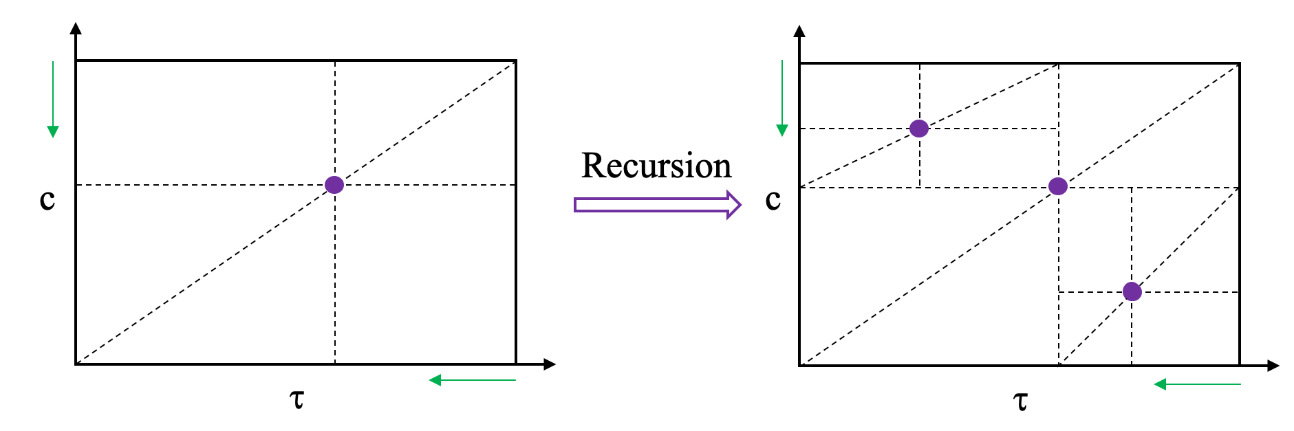 Figure 1
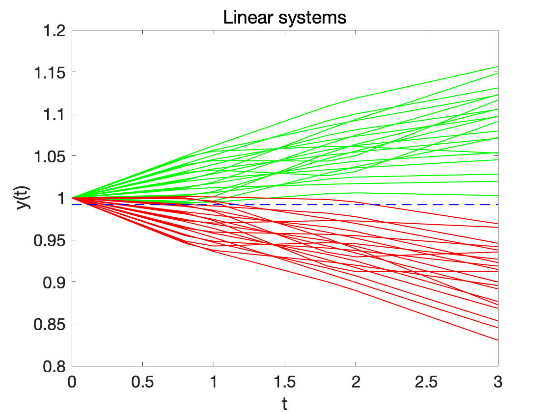 Figure 2
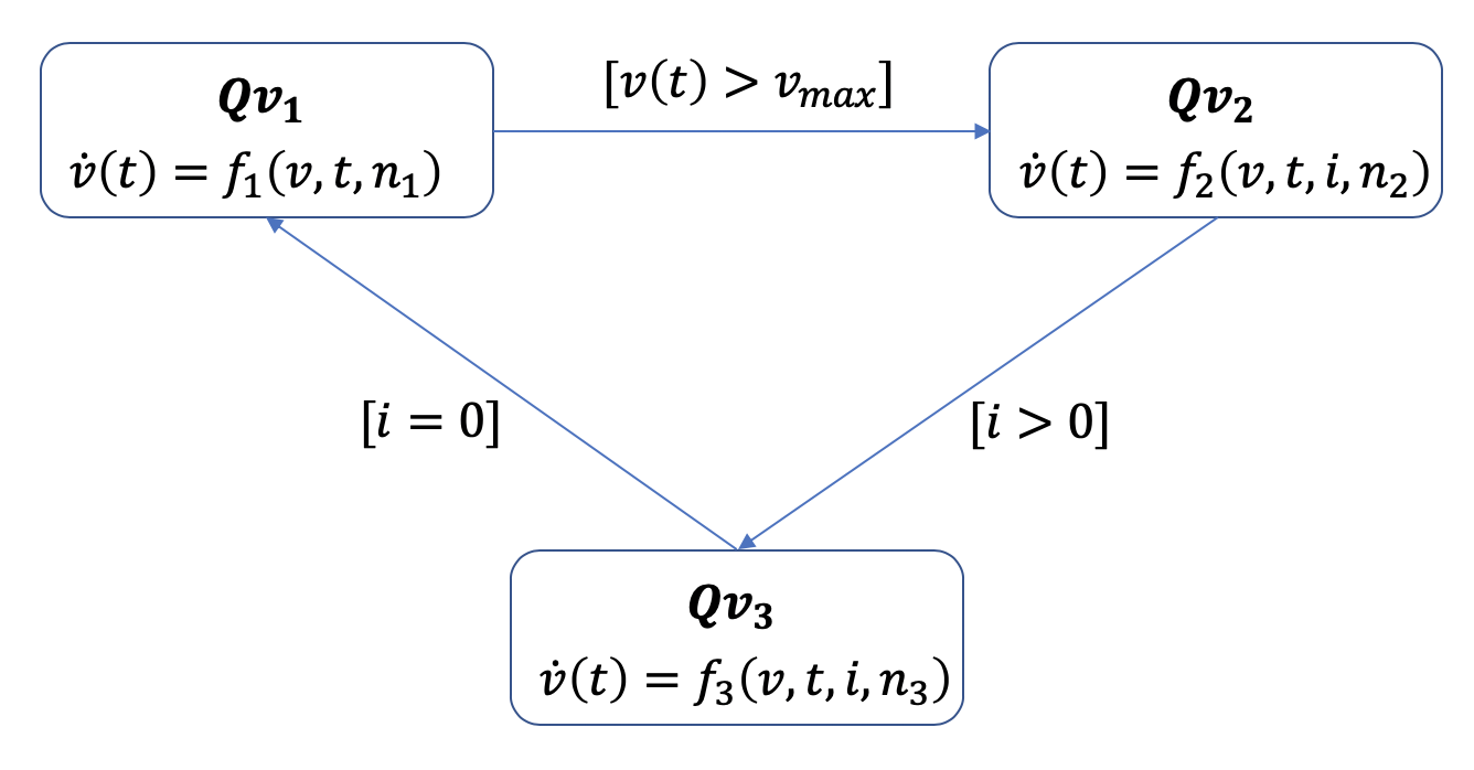 Figure 3
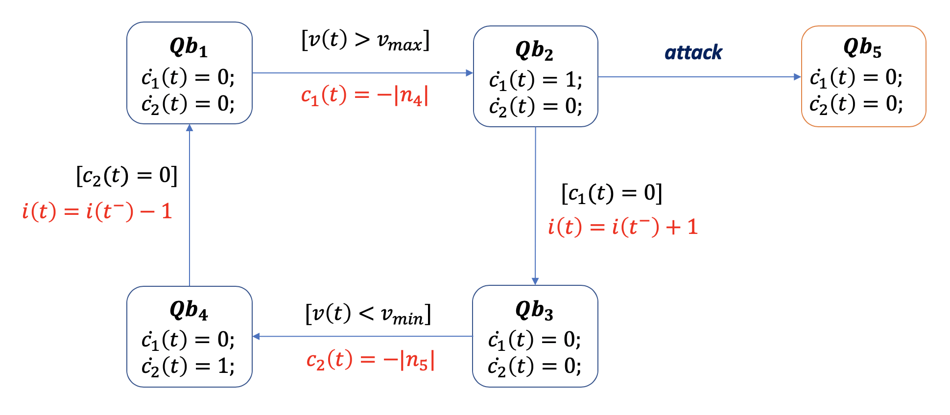 Figure 4
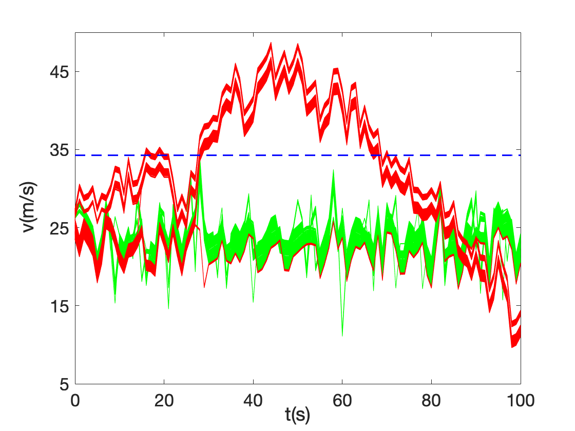 Figure 5
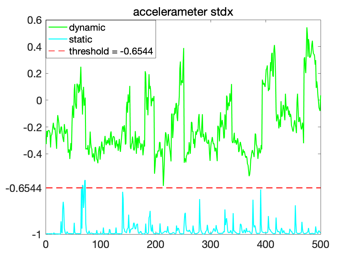 Figure 6
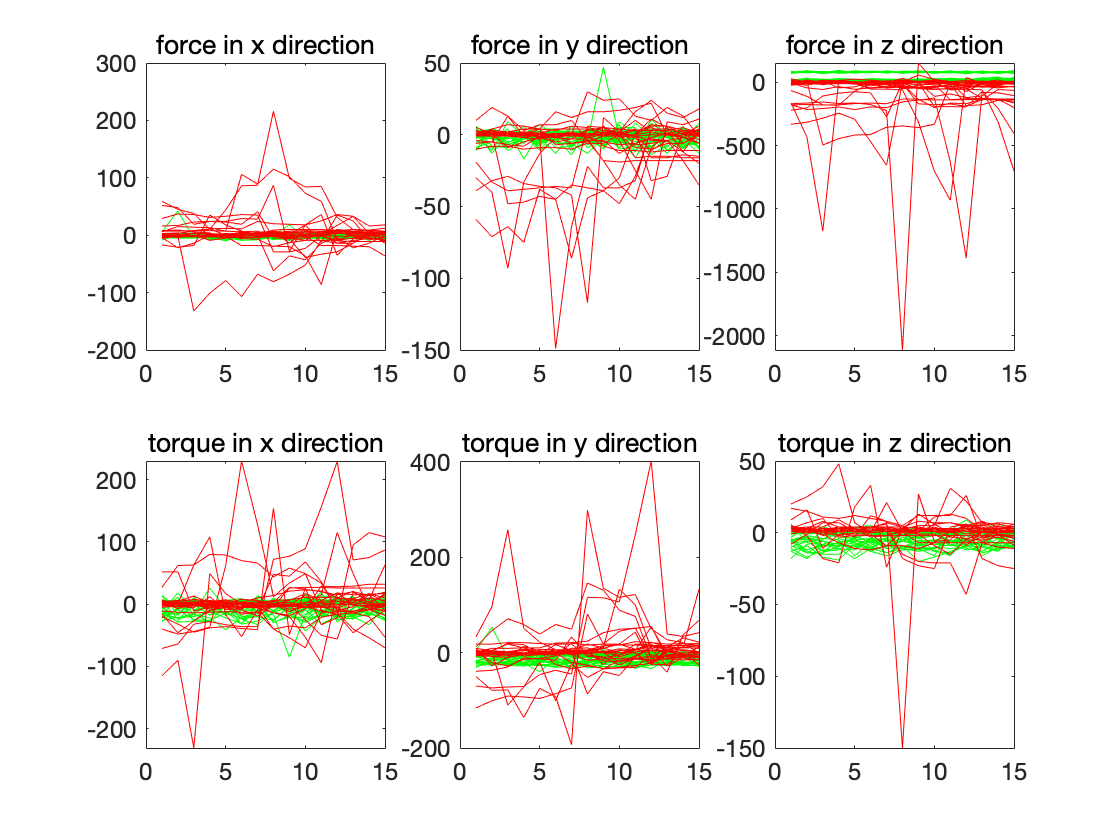 Figure 7
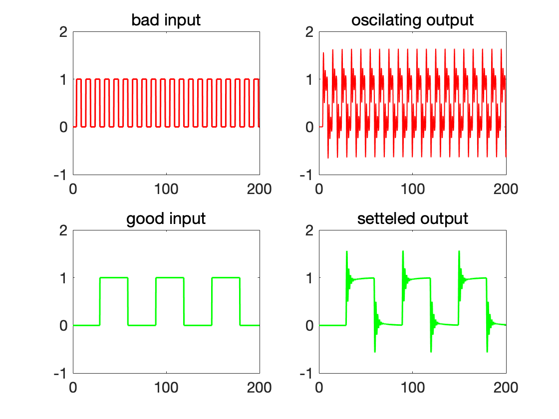 Figure 8
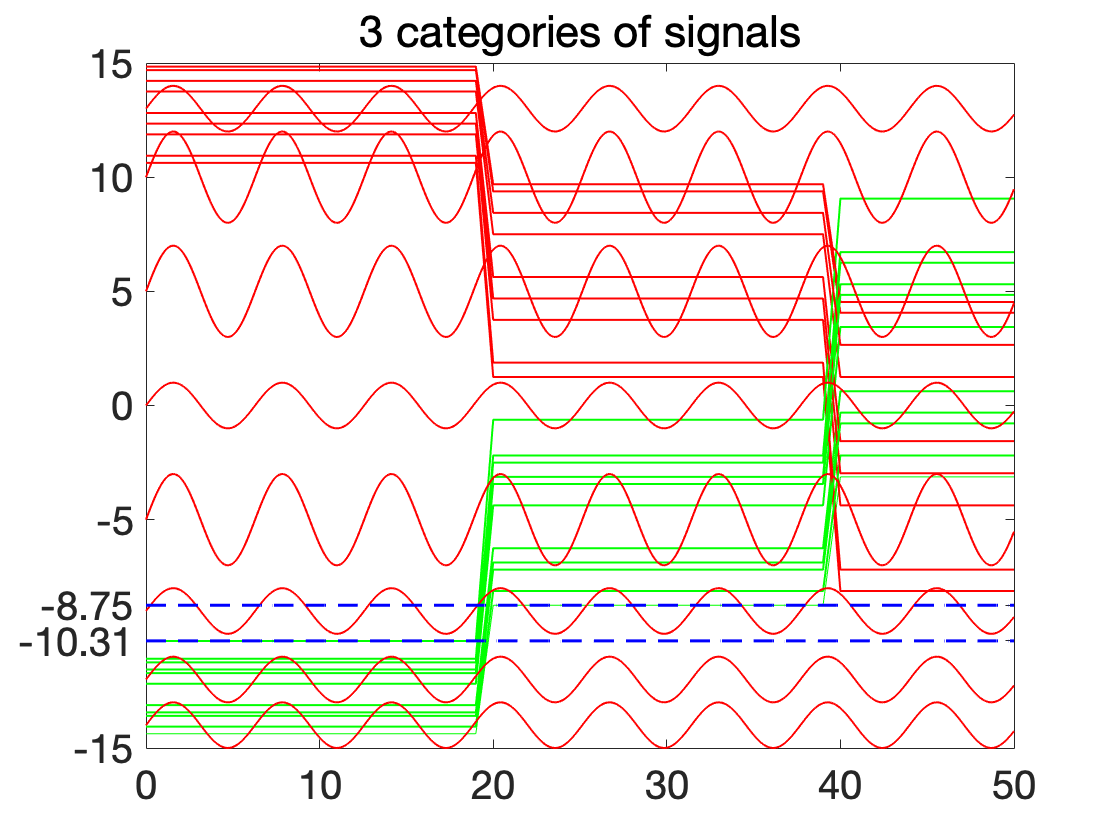 Figure 9
| Case | Before | After |
|---|---|---|
| optimization (s) | Optimization (s) | |
| Linear system | 44.25 | 39.05 |
| Cruise control of train | 35.84 | 32.31 |
| Human Activity Recognition | 28.06 | 22.07 |
| Robot execution failures | 29.64 | 27.91 |
| Environment assumption mining | 158.70 | 126.66 |
| Feature | STL classifier | Time before | Time after | MCR |
|---|---|---|---|---|
| optimization (s) | optimization (s) | |||
| 29.65 | 27.92 | 0.026 | ||
| 26.69 | 26.54 | 0.078 | ||
| 30.95 | 28.64 | 0.078 |
Peer Reviews
No public reviews on file for this paper yet. If you reviewed it on a platform where reviews are public (OpenReview, ICLR, NeurIPS, ICML), you can paste yours below so the community can read it here.
Videos
No videos yet. Explain this paper in a talk, walkthrough, or lecture? Add one.
Interpretable Classification of Time-Series Data using Efficient Enumerative Techniques
Sara Mohammadinejad
University of Southern California
&Jyotirmoy V. Deshmukh
University of Southern California
&Aniruddh G. Puranic
University of Southern California
&Marcell Vazquez-Chanlatte
University of California, Berkeley
&Alexandre Donzé
Decyphir, Inc
Abstract
Cyber-physical system applications such as autonomous vehicles, wearable devices, and avionic systems generate a large volume of time-series data. Designers often look for tools to help classify and categorize the data. Traditional machine learning techniques for time-series data offer several solutions to solve these problems; however, the artifacts trained by these algorithms often lack interpretability. On the other hand, temporal logics, such as Signal Temporal Logic (STL) have been successfully used in the formal methods community as specifications of time-series behaviors. In this work, we propose a new technique to automatically learn temporal logic formulae that are able to cluster and classify real-valued time-series data. Previous work on learning STL formulas from data either assumes a formula-template to be given by the user, or assumes some special fragment of STL that enables exploring the formula structure in a systematic fashion. In our technique, we relax these assumptions, and provide a way to systematically explore the space of all STL formulas. As the space of all STL formulas is very large, and contains many semantically equivalent formulas, we suggest a technique to heuristically prune the space of formulas considered. Finally, we illustrate our technique on various case studies from the automotive, transportation and healthcare domain.
1 Introduction
Cyber-physical systems (CPS) generate large amounts of data due to a proliferation of sensors responsible for monitoring various aspects of the system. Designers are typically interested in extracting high-level information from such data but due to its large volume, manual analysis is not feasible. Hence a crucial question is: How do we automatically identify logical structure or relations within CPS data? Machine learning (ML) algorithms may not be specialized to learn logical structure underlying time-series data[1], and typically require users to hand-create features of interest in the underlying time-series signals. These methods then try to learn discriminators over feature spaces to cluster or classify data. These feature spaces can often be quite large, and ML algorithms may choose a subset of these features in an ad hoc fashion. This results in an artifact (e.g., a discriminator or a clustering mechanism) [2] that is not human-interpretable. In fact, ML techniques focus only on solving the classification problem and suggest no other comprehension of the target system [3].
Signal Temporal Logic (STL) is a popular formalism to express properties of time-series data in several application contexts, such as automotive systems [4, 5, 6], analog circuits [7], biology [8], robotics [9], etc. STL is a logic over Boolean and temporal combinations of signal predicates which allows human-interpretable specification of continuous system requirements. For instance, in automotive domain, STL can be used to formulate properties such as “the car successfully stops before hitting an obstruction” [10].
There has been significant work in learning STL specifications from data. Some of this work has focused on supervised learning (where given labeled traces, an STL formula is learned to distinguish positively labeled traces from negatively labeled traces), or clustering (where signals are clustered together based on whether they satisfy similar STL formulas), or anomaly detection (where STL is utilized for recognizing the anomalous behavior of an embedded system). There are two main approaches in learning STL formulas from data: template-free learning and template-based learning. Template-free methods learn both the structure of the underlying STL formula and the formula itself. While these techniques have been proven effective for many diverse applications [2, 10, 3], they typically explore only a fragment of STL, and may produce long and complicated STL classifiers. Certain properties such as concurrent eventuality, repeated patterns and persistence may not be expressible in the chosen fragments for learning [10]. In template-based methods, the user provides a template parametric STL formula (PSTL formula) and the learning algorithm infers only the values of parameters from data [1, 11, 12, 13, 14]. Without a good understanding of the application domain, choosing the appropriate PSTL formula can be challenging. Furthermore, in template-based methods the users may provide very specific templates which may make it difficult to derive new knowledge from data[3].
Syntax-guided synthesis is a new paradigm in “learning from examples”, where the user provides a grammar for expressions, and the learning algorithm tries to learn a concise expression that explains a given set of examples. In [15], systematic enumeration has been used to generate candidate solutions. For medium-sized benchmarks, the systematic enumeration algorithm, in spite of its simplicity, surprisingly outperforms several other learning approaches [16].
Inspired by the idea of learning expressions from grammars, in this paper, we consider the problem of learning STL based formulas to classify a given labeled time-series dataset. The key challenge in systematic enumeration for STL is that predicates over real-valued signals and time-bounds on temporal operators both involve real numbers. This means that even for a fixed length, there are an infinite number of STL formulas of that length. One solution is to apply the enumerative approach to PSTL, which uses parameters instead of numbers. The inference problem then tries to learn parameter values to separate labeled data into distinct classes. The parameter-valuation inference procedures are typically efficient, but over a large dataset, the cost for enumeration followed by parameter inference can add up. As a result, we explore an optimization which involves skipping formulas that are heuristically determined to be equivalent.
As a concrete application of enumerative search, we consider the problem of learning an STL-based classifier with a minimal mis-classification rate for the given labeled dataset.
To summarize, our key contributions are as follows:
- •
We extend the work in [1, 11, 12, 13, 14] by learning the structure or template of PSTL formulas automatically. The enumerative solver furthers the Occam’s razor principle in learning (simplest explanations are preferred). Thus, it produces simpler STL formulas compared to existing template-free methods [2, 10, 3].
- •
We introduce the notion of formula signature as a heuristic to prevent enumeration of equivalent formulas.
- •
We bridge formal methods and machine learning algorithms by employing STL, which is a language for formal specification of continuous and discrete system behaviors [17]. We use Boolean satisfaction of STL formulas as a formal measure for measuring the mis-classification rate.
- •
We showcase our technique on real world data from several domains, including automotive, transportation and healthcare domain.
2 Preliminaries
Definition 2.1** (Time-Series, Traces)**
A trace is a mapping from time domain to value domain , where, , and .
**Signal Temporal Logic (STL). ** Signal Temporal Logic [17] is used as a specification language for reasoning about properties of real-valued signals. The simplest properties or constraints can be expressed in the form of atomic predicates. An atomic predicate is formulated as , where is a function from to , , and . For instance, is an atomic predicate, where , is , and . Temporal properties include temporal operators such as (always), (eventually) and (until). For example, means signal is always greater than 2. Each temporal operator is indexed by an interval , where . Every STL formula is written in the following form:
[TABLE]
where . and operators are special instances of operator , and , and they are defined for formula simplification. The boolean semantics of an STL formula are defined formally as follows:
[TABLE]
is the shorthand of . The signal satisfies at time (where if . It satisfies if for all time and satisfies if exists , such that and . The signal satisfies the formula if there exists some time where and , and for all time . We can create higher-level STL formulas by utilizing two or more of the operators. For instance, a signal satisfies iff there exists such that , and for all time .
In addition to the Boolean semantics, quantitative semantics of STL quantify the robustness degree of satisfaction by a particular trace[18, 19]. Intuitively, a STL with a large positive robustness is far from violation, and with large negative robustness is far from satisfaction. If the robustness is a small positive number, a very small perturbation might make it negative and lead to the violation of the property. Quantitative semantics of STL are formally defined as follow:
[TABLE]
For example, for STL formula the robustness value is , and for the robustness is . Property "Always between time 0 and some unspecified time , the signal is less than some value " could be expressed using Parametric STL (PSTL) , where the unspecified values and are referred to as parameters.
**Parametric Signal Temporal Logic (PSTL). ** PSTL [20] formula is an extension of STL formula where constants are replaced by parameters. The associated STL formula is obtained by assigning a value to each parameter variable using a valuation function. Let be the set of parameters, represent the domain set of the parameter variables , and represent the time domain of the parameter variables . Then is the set containing the two disjoint sets and , where at least one of the sets is non-empty. A valuation function maps a parameter to a value in its domain. A vector of parameter variables is obtained by mapping parameter vectors into tuples of respective values over or . Hence, we obtain the parameter space .
An STL formula is obtained by pairing a PSTL formula with a valuation function that assigns a value to each parameter variable. For example, consider the PSTL formula with parameters and . The STL formula which is an instance of is obtained with the valuation .
Definition 2.2** (Monotonic PSTL)**
A parameter is said to be monotonically increasing or have positive polarity in a PSTL formula if condition (2) holds for all , and is said to be monotonically decreasing or negative polarity if condition (3) holds for all , and monotonic if it is either monotonically increasing or decreasing [20].
[TABLE]
For example, in the formula , polarity of is positive (the formula is monotonically increasing with respect to ), and polarity of is negative (the formula is monotonically decreasing with respect to ).
Definition 2.3** (Validity domain)**
The validity domain for a given set of parameters is the set of all valuations s.t. for the given set of traces , each trace satisfies the STL formula obtained by instantiating the given PSTL formula with the parameter valuation. The boundary of the validity domain is the set of valuations where the robustness value of the given STL formula with respect to at least one trace in is [math].
Essentially, the validity domain boundary serves as a classifier to separate the set of traces satisfying the STL formula from the ones violating the formula.
**Supervised Learning/Classification. ** Supervised Learning is an ML technique used for learning from labeled data set. Supervised classification problems are either binary (only two classes are involved) or multi-class classification (more than two classes are included). In this paper, we explore the problem of binary classification for time-series data and use boolean semantics of STL as a logical measure for misclassification rate (MCR). In general, MCR is computes as the number of falsely classified traces divided by the number of all traces. We then evaluate our method on real-world data, including automotive, transportation and healthcare domain.
3 Enumerative Learning for STL
In this section, we introduce systematic PSTL enumeration for learning PSTL formula classifiers from time-series data, which the enumeration procedure is formalized in Algo. 1. From a grammar-based perspective a PSTL formula can be viewed as atomic formulas combined with unary or binary operators. For instance, PSTL formula consists of binary operator , unary operators and , and atomic predicates and .
[TABLE]
Algo. 1 is algorithm with several nested iterations. The outermost loop iterates over the length of the formula, and in the first iteration of the loop, we basically enumerate formulas of length , or parameterized signal predicates using the EnumAtoms function. At end of the iteration of the algorithm, all formulas up to length are stored in a database that is an array of lists. Each array index corresponds to the formula length, and each of the lists stored at location is the list of all formulas of length . In each iteration corresponding to lengths greater than , the algorithm calls the function ApplyUnaryOps, and in all iterations for lengths greater than , the function also calls ApplyBinaryOps. When enumerating formulas of length , ApplyUnaryOps function iteratively applies each unary operator from the ordered list unaryOps to all formulas of length to get a new formula. The ApplyBinaryOps iteratively applies each binary operator from the ordered list binaryOps to a pair of formulas of lengths and , where and . We use atomIt, unOpIt, binaryOpIt, argIt, lhsIt, rhsItas iterators (indices) on the lists atoms, unaryOps, binaryOps, , and lhsArgs and rhsArgs respectively.
For each PSTL formula generated by Algo. 2, we apply the procedure (). If is a good classifier (small misclassification rate), all loops terminate and is returned. Otherwise, the procedure continues to generate new PSTL formulas. We explain Algo. 2 in Section 5.
In order to avoid applying Algorithm 2 () on equivalent PSTL formulas, we use the idea of formula signatures to heuristically detect equivalent PSTL formulas. We explain this optimization in the next section.
4 Signature-based Optimization
Enumerating logical binary classification, which is implemented in Algorithm 2, for every PSTL formula is time-consuming. The problem with naïve enumeration approach for PSTL formulas is that many equivalent PSTL formulas are enumerated. Hence, we are interested in detecting equivalent PSTL formulas in order to decrease enumeration time. However, checking equivalence of PSTL formulas is in general undecidable [12]. Even if we restrict ourselves to a fragment of PSTL, equivalence checking is a computationally demanding task. Thus, we use signatures to avoid enumerating logically equivalent formulas. A signature is an approximation of an STL formula. Inspired by polynomial identity testing [21], we use the notion of signature to check the equivalence of two STL formulas. Let be a randomly chosen subset of (the traces) of cardinality . Let be a finite subset of (the parameter space). The signature of a formula maps to a matrix of real numbers, defined as below:
[TABLE]
The element of the matrix represents the robustness of the trace, with respect to the PSTL formula . For checking the satisfaction of a STL specification by a trace we use Breach [22], a toolbox for verification and parameter synthesis of hybrid systems. This procedure is implemented in computeSignature function in Algorithm2. computeSignature function in Algorithm2 is used to detect whether an enumerated PSTL formula is new or its equivalent has been enumerated.
Using the idea of signatures reduced the computation time in targeted case studies; the summary of the results are shown in Table 1. More explanation about computing signature for each case will be provided in Sec. 6. As Table 1 shows, the computation time difference before and after optimization is noticeable, yet, it is at best 22%. The reason is that the enumerative solver produces simple STL classifiers in 5 case studies, and until reaching those STL classifiers, only a few formulas with equivalent signatures are enumerated. For producing complicated classifiers, the difference would be more noticeable.
5 Logical Binary Classification
Next, we explain how to learn a logical and interpretable classifier for binary classification. We assume that we are given two sets of traces (those with label [math]) and (those with label ). The main steps in the algorithm are as follows:
The function checks whether the PSTL formula produced by Algo. 1 is heuristically equivalent to an existing formula. Internally, this is done by checking if the signature of the new formula is identical to the signature of an existing formula in the database of formulas, i.e. . In the next step, algorithm tries to obtain a point on the satisfaction boundary of the enumerated formula that results in a formula that serves as a good classifier. To explain this procedure further, we first recall the algorithm to approximate the satisfaction boundary of a given formula .
First we recall from [11] that the satisfaction boundary of a formula with respect to a set of traces is essentially the set of parameter valuations where the robustness value of for at least one trace is [math], i.e. the formula is marginally satisfied by at least one trace in .
In general, computing the satisfaction boundary for arbitrary PSTL formulas is difficult; however, for formulas in the monotonic fragment of PSTL [11], there is an efficient procedure to approximate the satisfaction boundary [23]. The procedure in [23] recursively approximates the satisfaction boundary to an arbitrary precision by performing binary search on diagonals of sub-regions within the parameter space. The idea is that in an -dimensional parameter space, a parameter valuation on the diagonal corresponds to a formula with zero robustness value. This point subdivides the parameter space into distinct regions: one where all valuations correspond to formulas that are valid over all traces, one where all valuations correspond to formulas that are invalid, and regions where satisfaction is unknown. The algorithm then proceeds to search along the diagonals of these remaining regions. This approximation results in a series of overlapping axis-aligned hyper-rectangles guaranteed to include the satisfaction boundary [11]. More details of this procedure can be found in [23]. We visualize an instance of the method in Fig. 1.
We combine the procedure from [23] with a classification algorithm as follows. In each recursive iteration of the multi-dimensional binary search, the algorithm identifies a point on the satisfaction boundary of with respect to the -labeled traces, i.e. . Let this point be denoted , and the resulting STL formula be denoted as in short-hand. We then check the Boolean satisfaction of on the traces in . The mis-classification rate (MCR) is computed as follows:
[TABLE]
If MCR is less than the specified threshold (threshold = in our implementation), the algorithm terminates, and is returned as the binary STL classifier for traces and . Otherwise, the algorithm goes to the next recursive computation of a boundary point (in another region of the parameter space). If the size of the parameter-space sub-region being searched (denoted by the variable in Algo. 2) exceeds a user-specified , the algorithm returns control to Algo. 1, which proceeds to enumerate the next PSTL formula for consideration.
Algo. 1 continues execution until a PSTL classifier with MCR threshold is found or the length of enumerated PSTL formula exceeds the maxLength defined by user, which means no PSTL classifier with MCR threshold can be found.
6 Case Studies
To evaluate the new framework, we apply our method on various case studies from the automotive, transportation and healthcare domain111We run the experiments on an Intel Core-i7 Macbook Pro with 2.7 GHz processors and 16 GB RAM.. The results show that the employed technique has a number of advantages compared to previous methods which are mentioned in section 7.
**Experiments on Synthetic data. ** We generated 28 synthetic traces (10 upward steps, 10 downward steps, and 8 sinusoids) in Fig. 2 in green and red colors. We are interested in categorizing green traces (upward steps) from red ones (downward steps and sinusoids). We applied our enumerative solver on these traces, and the resulting STL classifier is: , with and execution time = 4416.71 seconds. This STL classifier is compatible with the general behavior of upward steps. The blue dash lines in Fig. 2 show the thresholds of the learned STL formula ( and ). In this case study, a signature with and was used to detect the equivalent PSTL formulas. Of the 48 formulas enumerated, there was only one equivalent formula pruned by the signature-based equivalence check. This case study seeks to highlight an STL formula with a nested temporal operator.
**Linear System. ** We now compare our technique with another supervised learning technique, and for a fair comparison, we use the same models as [2]. We modeled the system whose dynamics evolve according to Eq. (LABEL:eqn:belta_lin_sys) shown in the Appendix. We generated 100 time-series traces of the system for the two different system modes, resulting in a total of 200 time-series traces. Fig. 3 shows the results of simulation. Green traces represent normal behaviors (absence of attack), and red traces represent the behavior of the system under attack. 50 of the data was split for training (50 normal and 50 anomaly), and the remaining data was reserved for testing. The enumerative solver was trained and tested on this data to extract an STL formula. The dashed blue line in the figure shows the threshold (=0.992) of the learned formula: . This is a simpler formula compared to the one obtained in [2], which is .
We use a marginally better computing platform than Jones et al., and our procedure takes 39.05s (with signature-based pruning) and 44.25s (without signatures), whereas the approach by Jones et al. required approximately 130s to extract the formula. We used a signature with and to detect equivalent PSTL formulas. In total, 5 formulas were enumerated, and we could prune 2 of them as logically equivalent to other enumerated formulas.
**Cruise Control of Train. ** We also benchmark an example for cruise control in a train from [2]. The system consists of a 3-car train, where each car has its own electronically-controlled pneumatic (ECP) braking mechanism. The velocity of the entire train is modeled as a single system. Hence, there are a total of 4 models (1 for velocity + 3 for braking in each car). The description of the velocity and ECP braking models can be found in the Appendix. The observations/readings of the train velocity is assumed to be noisy.
The cruising speed of the train is set to and the train oscillates about this speed by . Under normal conditions, the train maintains the cruising speed and applies its brakes when the speed exceeds a threshold/upper limit. In an anomalous situation (or attack), all the brakes fail to engage and hence the train fails to maintain its speed within the desired/set limits. The velocity parameters were set to be in the interval . For this system, we generated data from 200 simulations (100 for normal and 100 for anomaly behavior). The time-series data corresponding to the simulations is shown in Fig. 4, in which the green traces represent normal behaviors, while red traces represent anomalies. Since Breach [22] could possibly choose a low initial velocity during an anomaly situation, a very low percentage of the traces tend to exhibit normal behaviors, as seen from the figure. Similar to our previous approaches, the data was split 50 (50 normal and 50 anomaly traces) for training and the rest for testing.
We applied our solver to extract the STL formula: , where the threshold learned by our solver is 34.2579 (shown by the dashed blue line in the figure). The MCRs for training and testing are and respectively. The STL formula obtained by our approach is simpler compared to the one extracted in [2], which is: . The total time for learning the classifier in [2] 154s, while the execution time of our approach is 32.31s (with signatures) and 35.84s (without signatures). In this case study, a signature with and was used to detect the equivalent PSTL formulas. Of the 5 enumerated formulas, we used signatures to prune 2 formulas.
**Human Activity Recognition. **
The UC Irvine time-series learning repository contains time-series data for Human Activity Recognition from inertial sensors (such as accelerometers) in waist-mounted smartphones [24]. This data was obtained from the recordings of 30 subjects performing activities of daily living. Six basic activities were performed by human subjects: three static postures (standing, sitting, lying) and three dynamic activities (walking, walking downstairs and walking upstairs). In our experiments, we consider the classification of the data into the two postures: static and dynamic. This is an important task for healthcare professionals to monitor the activities and vital organs of people undergoing medication and the elderly. The time-series signals from the accelerometers are processed using certain filters. One of them computes the standard deviation of the acceleration in the direction in a certain time-window. We used this signal to study whether we can obtain STL classifiers.
A sampling of the corresponding data is shown in Fig. 5. 25 traces, each having a sampling rate of 50 samples per second for a total of 10 seconds, were used for training. 10 traces were used for testing. We were able to obtain an MCR of [math] on both the training and test data. The STL formula learned by the algorithm is: , where is the aforementioned standard deviation signal provided by the data. Current methods [25, 26, 27] achieve an accuracy of about 96%. Our solver was able to achieve an accuracy of 100%, which shows a significant improvement over current approaches [25, 26, 27]. Furthermore, our solver uses only 1 feature compared to [25], which uses 17 features. The time required for execution of the solver is 22.07 seconds (with signatures) and 28.06 seconds (without signatures).
While we find our results a significant improvement over the state-of-the-art in terms of accuracy and run-time, we comment that ML algorithms excel at being able to learn from large feature spaces, and choosing the right feature which is a challenging task. It would be interesting to benchmark our approach where we use all the signal variables in the data (and the possibly much larger space of formulas over the larger number of signals).
**Robot Execution Failures. **
The robot execution failures dataset contains force and torque measurements along the 3 axes (x, y and z) of an assembly (pick-and-place) robot after detecting a failure [24]. force/torque samples collected at regular time intervals characterize each failure. It consists of 5 datasets of failures in the following tasks: approach to grasp position, transfer of a part, position of part after a transfer failure, approach to ungrasp position and in motion with part. The dataset is obtained from the UCI Machine Learning repository at [28]. In our experiments, we use the two of the datasets of robot failures, which are described as follows.
Dataset LP2: Failures in transfer of a part. This dataset consists of 88 traces and contains classes representing normal, collision, front collision and obstruction behaviors. For our experiment, we used the 21 traces that exhibit normal behavior and 17 traces that exhibit collision, and applied our solver to classify the traces into these two groups. The results of our solver are shown in Table 2. In [29], their best algorithm had an accuracy of 68% which uses Fourier transform of force and torque in three direction of x, y, and z. Our solver shows a major improvement in accuracy as the misclassification rate is less than 0.1%, by using only one feature from raw data. The result STL classifiers using each of the three features , , and are shown in Table 2.
Dataset LP5: Failures in motion with part. This dataset consists of 164 instances, of which 44 instances exhibit normal behavior and 26 instances exhibit bottom collision. The dataset containing these traces are shown in Fig. 6 in which the green traces indicate normal behaviors, while the red traces indicate collisions. We used the same approach as for the LP2 dataset and our solver learned the STL , with a misclassification rate of 0. The processing time with signature is , while the processing time without signature is . In this case, the processing time without using signature is better; the reason is that until reaching the “always” temporal logic operator, we only encounter two repetitive formulas which are atomic predicates and for which, the processing times are very small, while the times required to compute the signature are greater. Therefore, signature is more effective when the length of the formula and number of traces increase. In [29], their best algorithm had an accuracy of 77% which uses a long feature vector. Our solver, with 0% misclassification rate by using only 1 feature shows a remarkable improvement compared to [29].
**Environment Assumption Mining. ** Given a deterministic system and a specification , the goal of assumption mining is to determine the subset of initial states or inputs that ensure satisfaction of an STL formula on the output of the model. In other words, we want to know what STL formulas do the inputs satisfy that guarantee that the outputs will be desirable. In our experiments, we try to learn the STL formulas that separates good inputs from bad inputs. For our experiment, we consider a PID controller for a damped second-order continuous system. The desired output of this system is to observe that the output has settled or is oscillating. We use 31 input traces with periods: 10, 12, 14, …, 70 and their negations. The traces are shown in Fig. 7. For oscillating outputs, the STL formula learned by the solver is: . It means for periods below , the output does not settle. This is to be expected, as this period is less than the settling time of the system. The time required for learning is 126.66s (with signatures) and is 158.70s (without signatures). In this case, and were chosen as dimensions of signature. Among total of 11 formulas enumerated, signatures could prune 4 equivalent formulas.
7 Related Works
There has been considerable recent work on learning STL formulas from data for various applications such as supervised learning [3, 10], clustering [1, 11], or anomaly detection[2].
In [10], a fragment of PSTL (rPSTL or reactive parametric signal temporal logic) is defined to capture causal relationships from data. However, there are some temporal properties namely, concurrent eventuality and nested always eventually that cannot be described directly in rPSTL. In [2], the authors extend [10] by using a fragment of rPSTL, inference parametric STL (iPSTL), that does not require a causal structure. In this work, classical ML algorithms (one-class support vector machines) are applied for unsupervised learning problem. In [3], a decision tree based method is employed to learn STL formulas, which creates a map between a restricted fragment of STL and a binary decision tree in order to build a STL classifier. While this seminal work has advanced work in the intersection of formal methods and machine learning, one disadvantage of these approaches has been that they lead to long formulas which can become an issue for interpretability.
In template-based techniques, a fixed PSTL template is provided by the user, and the techniques only learn the values of parameters associated with the PSTL. In [1], a total ordering on parameter space of PSTL specifications is utilized as feature vectors for learning logical specifications. Unfortunately, recognizing the best total ordering is not straightforward for users. In [11], the authors eliminate this additional burden on the user by suggesting a method that maps timed traces to a surface in the parameter space of the formula, and then employing these curves as features. In [12], the input to the algorithm is a requirement template expressed in PSTL, where the traces are actively generated from a model of the system. Our proposed technique, which uses systematic enumeration, can produce smaller formulas which may be more human-interpretable, and with higher accuracy( in all investigated case studies).
8 Conclusion
We proposed a new technique for binary classification of time-series data using Signal Temporal Logic formulas. The key idea is to combine an algorithm for systematic enumeration of PSTL formulas with an algorithm for estimation of the satisfaction boundary of the enumerated PSTL formula. We also investigate an optimization using formula signatures to avoid enumerating equivalent PSTL formulas. We then illustrate this technique with a number of case studies on real world data from different domains. The results show that the enumerative solver has a number of advantages. As future work, we will extend this approach to multi-class classification, unsupervised, semi-supervised, and active learning. We will also investigate other optimization techniques to make the enumerative solver faster and more memory-efficient.
The reference list from the paper itself. Each links out to its DOI / PubMed record.
- 1[1] Marcell Vazquez-Chanlatte, Jyotirmoy V Deshmukh, Xiaoqing Jin, and Sanjit A Seshia. Logical clustering and learning for time-series data. In International Conference on Computer Aided Verification , pages 305–325. Springer, 2017.
- 2[2] Austin Jones, Zhaodan Kong, and Calin Belta. Anomaly detection in cyber-physical systems: A formal methods approach. In 53rd IEEE Conference on Decision and Control , pages 848–853. IEEE, 2014.
- 3[3] Giuseppe Bombara, Cristian-Ioan Vasile, Francisco Penedo, Hirotoshi Yasuoka, and Calin Belta. A decision tree approach to data classification using signal temporal logic. In Proceedings of the 19th International Conference on Hybrid Systems: Computation and Control , pages 1–10. ACM, 2016.
- 4[4] James Kapinski, Xiaoqing Jin, Jyotirmoy Deshmukh, Alexandre Donze, Tomoya Yamaguchi, Hisahiro Ito, Tomoyuki Kaga, Shunsuke Kobuna, and Sanjit Seshia. St-lib: a library for specifying and classifying model behaviors. Technical report, SAE Technical Paper, 2016.
- 5[5] Xiaoqing Jin, Jyotirmoy V Deshmukh, James Kapinski, Koichi Ueda, and Ken Butts. Powertrain control verification benchmark. In Proceedings of the 17th international conference on Hybrid systems: computation and control , pages 253–262. ACM, 2014.
- 6[6] Ayca Balkan, Paulo Tabuada, Jyotirmoy V Deshmukh, Xiaoqing Jin, and James Kapinski. Underminer: A framework for automatically identifying nonconverging behaviors in black-box system models. ACM Transactions on Embedded Computing Systems (TECS) , 17(1):20, 2018.
- 7[7] Oded Maler and Dejan Ničković. Monitoring properties of analog and mixed-signal circuits. International Journal on Software Tools for Technology Transfer , 15(3):247–268, 2013.
- 8[8] Szymon Stoma, Alexandre Donzé, François Bertaux, Oded Maler, and Gregory Batt. Stl-based analysis of trail-induced apoptosis challenges the notion of type i/type ii cell line classification. P Lo S computational biology , 9(5):e 1003056, 2013.