Asymptotically exact unweighted particle filter for manifold-valued hidden states and point process observations
Simone Carlo Surace, Anna Kutschireiter, Jean-Pascal Pfister

TL;DR
This paper introduces an asymptotically exact particle filter for manifold-valued hidden states with point process observations, utilizing intrinsic dynamics and PDE-based control terms to improve filtering accuracy.
Contribution
It develops a novel filter (ppFPF) that extends feedback particle filtering to manifolds with point process data, using PDE solutions for control, ensuring intrinsic and accurate state estimation.
Findings
The filter accurately updates particles on manifolds during observations.
It leverages PDE solutions similar to weighted Poisson equations for control.
The method is compatible with existing PDE approximation algorithms.
Abstract
The filtering of a Markov diffusion process on a manifold from counting process observations leads to `large' changes in the conditional distribution upon an observed event, corresponding to a multiplication of the density by the intensity function of the observation process. If that distribution is represented by unweighted samples or particles, they need to be jointly transformed such that they sample from the modified distribution. In previous work, this transformation has been approximated by a translation of all the particles by a common vector. However, such an operation is ill-defined on a manifold, and on a vector space, a constant gain can lead to a wrong estimate of the uncertainty over the hidden state. Here, taking inspiration from the feedback particle filter (FPF), we derive an asymptotically exact filter (called ppFPF) for point process observations, whose particles…
Click any figure to enlarge with its caption.
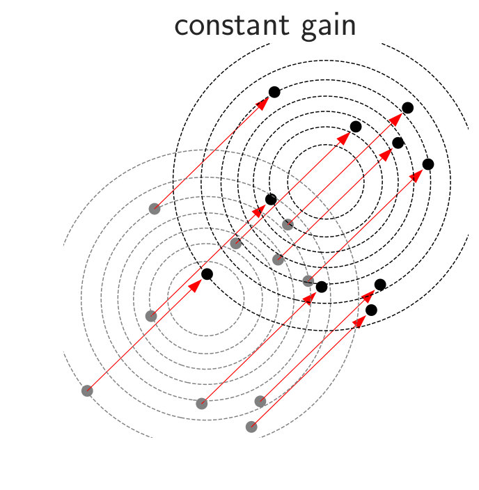 Figure 2
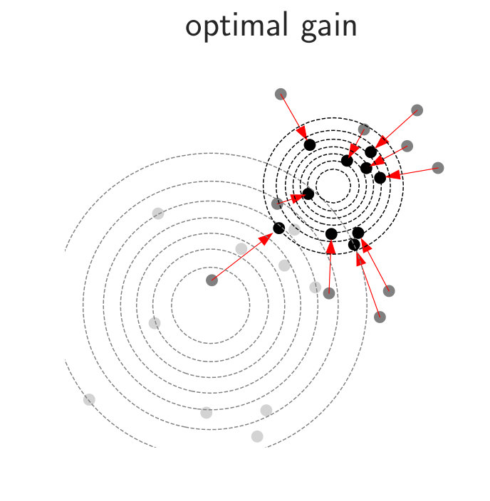 Figure 2
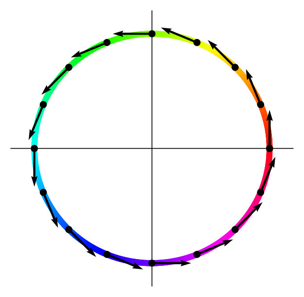 Figure 3
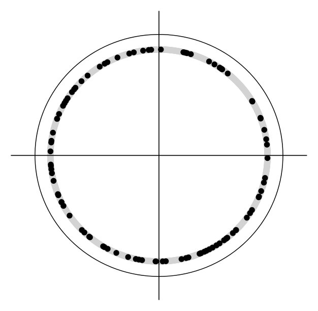 Figure 4
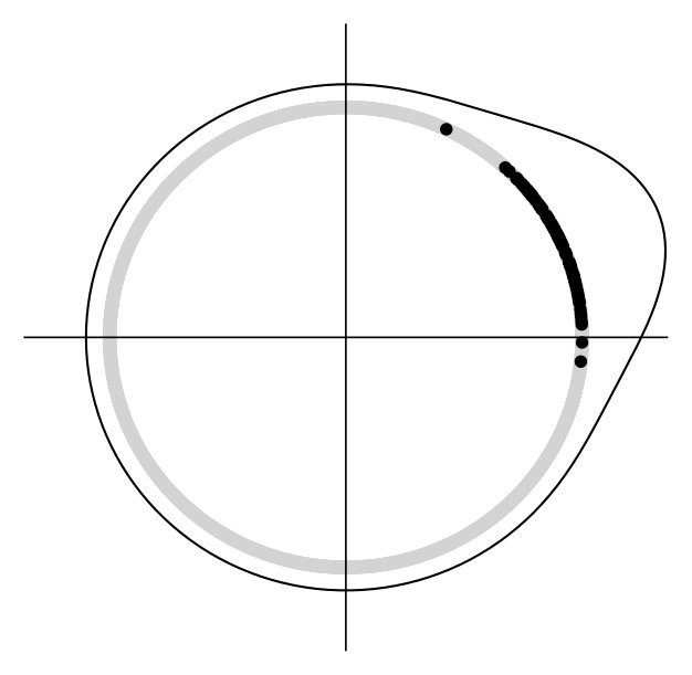 Figure 5
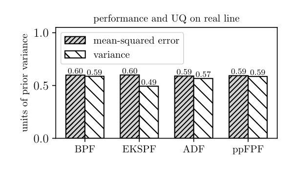 Figure 6
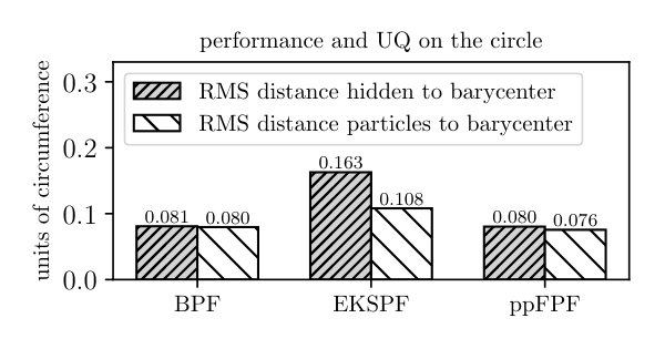 Figure 7
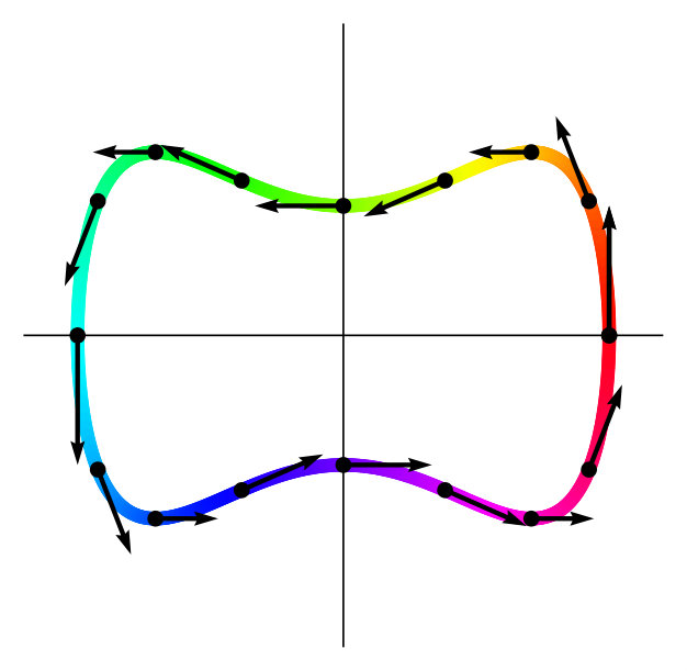 Figure 8
Peer Reviews
No public reviews on file for this paper yet. If you reviewed it on a platform where reviews are public (OpenReview, ICLR, NeurIPS, ICML), you can paste yours below so the community can read it here.
Videos
No videos yet. Explain this paper in a talk, walkthrough, or lecture? Add one.
Asymptotically exact unweighted particle filter for manifold-valued hidden states and point process observations
Simone Carlo Surace*†, Anna Kutschireiter†,∗, Jean-Pascal Pfister†,∘* *†*Department of Physiology, University of Bern, Switzerland. *∗*Department of Neurobiology, Harvard Medical School, Boston MA, USA. *∘*Institute of Neuroinformatics, University and ETH Zurich, Switzerland. This work was supported by the Swiss National Science Foundation, grant PP00P3_179060. Corresponding author: [email protected]
Abstract
The filtering of a Markov diffusion process on a manifold from counting process observations leads to ‘large’ changes in the conditional distribution upon an observed event, corresponding to a multiplication of the density by the intensity function of the observation process. If that distribution is represented by unweighted samples or particles, they need to be jointly transformed such that they sample from the modified distribution. In previous work, this transformation has been approximated by a translation of all the particles by a common vector. However, such an operation is ill-defined on a manifold, and on a vector space, a constant gain can lead to a wrong estimate of the uncertainty over the hidden state. Here, taking inspiration from the feedback particle filter (FPF), we derive an asymptotically exact filter (called ppFPF) for point process observations, whose particles evolve according to intrinsic (i.e. parametrization-invariant) dynamics that are composed of the dynamics of the hidden state plus additional control terms. While not sharing the gain-times-error structure of the FPF, the optimal control terms are expressed as solutions to partial differential equations analogous to the weighted Poisson equation for the gain of the FPF. The proposed filter can therefore make use of existing approximation algorithms for solutions of weighted Poisson equations.
Index Terms:
Filtering, Estimation, Stochastic systems, Mean field games, Stochastic optimal control
I Introduction
Alarge number of natural and engineered systems and datasets have states that are naturally described as elements of smooth manifolds. Classical cases are the motion of a body constrained by equality constraints, motion on the surface of the earth, or the attitude of a rigid body. Increasingly, the systems are very high-dimensional, whereas data points often lie on relatively low-dimensional manifolds, whose structure can be exploited for filtering and estimation problems.
In filtering, the state of the system (called the hidden state) needs to be estimated from the history of observations. In practise, observations often arrive sparsely, randomly and in digital form. One example is when observations are simple event counts. Such counting or point process observations arise in a variety of applications of time series models, e.g. neuroscience, geosciences, or finance.
The exact solution of the filtering problem is intractable in most cases and requires numerical approximation. One approach has been the class of interacting particle algorithms, in which an unweighted ensemble of particles is propagated based on the known dynamics of the hidden state and the incoming observations. The feedback particle filter (FPF) [1]-[2] is such an algorithm that is based on mean-field optimal control, with a gainerror structure that is reminiscent of the Kalman filter. The gain is given by the solution of a partial differential equation (PDE), which makes the FPF exact in the limit of large even for nonlinear problems. Although in practise the gain has to be estimated from the particles, unweighted approaches hold the promise of scaling to high-dimensional problems, in contrast to particle algorithms with importance weights [3].
In this paper, we consider the problem of finding an FPF-like algorithm for systems whose hidden states evolve continuously in time on a known smooth manifold and observations are given by a conditional Poisson process. The FPF for manifold-valued hidden states and diffusion observations has been introduced in [4]. A filter for a hidden state in and point process observations was introduced in [5], called EKSPF. While it is reminiscent of the FPF, having a gainerror structure, it uses a constant gain. As a result, the filter is exact only to first order and does not properly reflect higher-order statistics. For example, when particles are initially spread out and an incoming event confers evidence that the hidden state is in some narrow region of the state space, we should find the updated particles concentrated in that region. However, upon an event the EKSPF translates all particles by the same vector, see Figures 1-1.
The reliance on this uniform translation also leads to difficulties in extending the EKSPF to hidden states evolving on a manifold. In fact, when the EKSPF is applied naïvely on some arbitrary chart of the manifold, filtering performance can be poor (see Section IV for an example). This is because the meaning of a ‘translation’ is fundamentally ill-defined on a manifold. Since a translation in coordinate chart does not necessarily correspond to a translation in coordinate chart , the performance of the EKSPF depends on the choice of coordinates. However, the filtering problem on a manifold is intrinsic, i.e. independent of the choice of coordinates. It would therefore be desirable for a particle filter, and the transformation of particles in particular, to be defined in a coordinate-independent way. This would be advantageous even if the state space carries additional structure, such as the vector space structure on . A large class of estimation problems in , such as e.g. satellite tracking, are naturally described in curvilinear coordinates.
For infinitesimal motion of particles, the notion of constancy of a vector field111As we will explain in the next section, the control terms in the FPF can be viewed as vector fields, and thus of a constant gain approximation, depends on additional structure on the manifold, namely a connection; a mathematical structure that prescribes how to parallel transport a vector between different points. This can be visualised for the example of the unit circle that (regarded as a smooth manifold) can be embedded in different ways in, say, (see Figures 1-1). If the constancy of a tangent vector field is made to depend on the embedding, then we obtain different vector fields for different embeddings. On many manifolds, there are no nontrivial parallel vector fields, which precludes the choice of a nontrivial constant gain. While this problem also affects a constant gain approximation of the FPF gain, the problem can be circumvented by seeking a non-constant gain estimate. Meanwhile, the constant gain assumption is ‘baked’ into the EKSPF.
In this paper, we derive an exact FPF-like filter on a manifold for point process observations, called ppFPF, from first principles, addressing the limitations of a constant gain in the EKSPF. The result is a filter whose control terms are given by solutions of PDEs analogous to the Poisson equation for the gain of the FPF. However, the gainerror structure of the FPF is not strictly preserved. Instead, for the conceptual reasons stated above, the control term associated to an event is fundamentally distinct and treated separately from the term in-between events.
The remainder of the paper is structured as follows: in Section II, we introduce the mathematical notation, review the filtering problem for the Gaussian white noise observation case, and re-derive the FPF in the manifold setting, making some observations regarding the symmetry of the problem. In Section III, we present our main contribution: we derive the ppFPF, which is an adaptation of the FPF to point-process observations. In Section IV, we present numerical examples that illustrate the differences in performance and uncertainty quantification (UQ) between the ppFPF and other filters.
\floatsetup
[figure]style=plain, subcapbesideposition=top
II Preliminaries and background
II-A Notations and conventions
Tangent vectors at a point are written in a local chart as , where Einstein’s summation convention is used. A vector field is a smooth section of the tangent bundle and is written locally as a first-order differential operator . The Lie derivative with respect to the vector field is denoted by and acts on sections of tensor product bundles of . If , then its differential is a one-form or smooth section of the cotangent bundle . More generally, a differential form of degree is a smooth section of , where the wedge denotes the exterior product. Top degree forms are elements of , where is the dimension of . A nowhere-vanishing element of is an orientation; if such an element exists then is called orientable, and we can then distinguish positive top degree forms, which we call volume forms. Normalized volume forms will be used to describe smooth nowhere-vanishing distributions on . The letter is used for exterior derivatives on differential forms as , and for stochastic differentials on stochastic processes as . The interior derivative on wrt. is written as . The notation is used for the filtration generated by the process .
II-B Filtering problem and filtering equations
We consider a filtering problem in which the hidden state evolves as a Markov diffusion process on an -dimensional manifold222To avoid further complications, we assume to be connected and orientable. , described by a Stratonovich stochastic differential equation (SDE) of the form
[TABLE]
in local coordinates, where are mutually independent standard Brownian motions.333We use Einstein’s summation convention. We will use the index-free notation for such an SDE on . This SDE corresponds to an infinitesimal generator
[TABLE]
where are vector fields on . This is a second-order differential operator, which can be expressed in local coordinates as .
The classical observation model in nonlinear filtering is a diffusion process with additive noise, also referred to as observations in Gaussian white noise, i.e.
[TABLE]
where is a Brownian motion independent of . Although the present paper is concerned with point process observations, in order to explain the background of this paper this section will focus exclusively on the model in Eq. (3). Later, in Section III, we shall consider point process observations, adapting an approach that has been used in the case of Gaussian white noise.
Probability distributions over the manifold will be described by positive top-degree forms (volume forms) that integrate to one, i.e. . This convention avoids the superfluous appearance of a reference measure on , and therefore emphasizes the metric-independent nature of the filtering problem. Of course, for concreteness, it is always possible to pick a reference volume form (for example, take the riemannian volume measure with respect to some riemannian metric on , e.g. the Lebesgue measure for ), and then to express in terms of a density as .
If the distribution of is described in terms of a volume form , the conditional distribution of , given observations , evolves according to the equation
[TABLE]
where and is the adjoint of with respect to the dual pairing of volume forms and smooth functions, i.e. for all bounded and all volume forms we have
[TABLE]
Eq. (4) is known as the Kushner-Stratonovich equation, see e.g. [6].
II-C Unweighted particle filters
In unweighted particle filtering, the goal is to find a Monte-Carlo approximation of , i.e. for any , the objective is to find processes , , called particles such that . The processes should be adapted to , where is a vector-valued process independent of and that can capture additional noise in the particle dynamics. Usually, one is interested in ‘symmetric’ particle representations in which all have identical distributions. The problem thus is to specify dynamics for a representative process that depend on the particle ensemble.
II-D Feedback particle filter
For Gaussian white noise observations, a recipe for building such a particle filter is known. Let us briefly review the derivation of the feedback particle filter (FPF) [2] (see [4] for the manifold setting). The FPF uses particle dynamics given by the prior dynamics plus a feedback control term that is chosen such that the Fokker-Planck equation for a single particle gives the same change in distribution as the filtering equation. An ansatz of gives
[TABLE]
where is an independent copy of . A corresponding equation for the conditional distribution of given , denoted by , can be derived by an integration-by-parts argument using Lie derivatives:
[TABLE]
In the first line, the Stratonovich chain rule is used. In the second line, directional derivatives are replaced by Lie derivatives444On smooth functions, the Lie derivative agrees with the directional derivative, i.e. for all ., and we performed integration by parts, reducing exact top-degree forms to boundary terms using Stokes’ theorem. It is customary to demand that be tangent to the boundary of (if is nonempty), or even completely vanish on . This assumption implies on , such that the boundary terms can be discarded. After switching back to Itô calculus, one obtains
[TABLE]
Matching the terms of Eq. (8) with Eq. (4) (conditioned on ) leads to the system of equations555 denotes the directional derivative of in the direction of the vector field , whereas is the vector field scaled point-wise by the function .
[TABLE]
Given a vector field solving Eq. (9), called a gain for the FPF, setting
[TABLE]
gives an associated solution to Eq. (10).666This can be shown by using Cartan’s magic formula and the graded product rule for the interior derivative, or simply by observing that for all , and .
II-E Uniqueness, approximation, and estimation of the gain
The solutions of Eqs. (9) and (10) are not unique, as any pair of solutions can be modified by adding an arbitrary divergence-free777The divergence of a vector field with respect to a volume form is the function defined implicitly by . Using Cartan’s magic formula and the fact that , the divergence can also be written as . It follows that for we have . vector field , i.e. such that . Uniqueness can be obtained by fixing a riemannian metric , and then demanding that the gain take the form . This leads to the equation . Moreover, if denotes the riemannian volume form and is expressed in terms of the density as , Eq. (9) reduces to a (weighted) Poisson equation
[TABLE]
Existence and uniqueness of a solution is guaranteed under mild assumptions on and (see [7], Theorem 2.2), and minimizes the functional among all solutions of Eq. (9) (see Lemma 8.4.2 in [8]). In the case , Euclidean , Gaussian , and linear , this gain reduces to the Kalman gain.
Sometimes it is desirable to approximate the vector field , where solves Eq. (12), by a constant. As mentioned in the introduction, in order to define the notion of constancy on a manifold, an additional structure , called connection, has to be defined. One may choose the Levi-Civita connection corresponding to some (already given) , but other choices are possible. A constant gain can then be defined as the minimum of over all parallel (i.e. ). For example, when , g is the Euclidean metric, and its Levi-Civita connection,
[TABLE]
The right-hand representation is obtained by multiplying the Eq. (12) by , integrating by parts, and using . Eq. (13) is convenient because the RHS can be estimated by a sample, but on some manifolds, topological obstructions make this approach infeasible. On with the standard metric and connection, a constant vector field cannot be a gradient of a smooth function. Insisting and performing the calculation on a chart leads to . It is unclear how to estimate the additional term that depends on the exact gain. In other cases the situation is still worse: many manifolds with connection do not have any nontrivial parallel vector fields (a common example is with its standard connection).
In practise, the gain has to be estimated from a finite number of particles , , thought to be i.i.d. samples from . If only the gain at the particle locations is needed, we denote the mapping particlesgains by , where and . This is called the gain estimation problem. For the purposes of this article, the question of how to optimally estimate the gain shall be left aside and we refer to e.g. [9, 10, 11] and the references therein. The aim is to show that the construction of an FPF-like algorithm for point processes can be fully reduced to the same types of equations as for the FPF gain, i.e. to equations of the following form:
Definition II.1
For every positive volume form with and every smooth function we denote by the equation
[TABLE]
whose unknown quantity is the vector field .
III FPF for point process observations
Now, we consider the case where the hidden state is a diffusion on a manifold as in Section II, but the observation process is now a counting process888By convention, is right-continuous with left limits (càdlàg). , counting the number of events since time , with intensity function , where is called the observation function. Here, the observations are corrupted by Poisson noise.
An equation for the optimal filter is known also in this setting. If the distribution of is described in terms of a volume form , the conditional distribution of given observations evolves according to the equation
[TABLE]
where denotes left limits. Eq. (15) will be referred to as the filtering equation for point process observations. It is sometimes called Kushner-Stratonovich-Poisson equation (see [5] for further references).
The goal of the present section is to carry out the derivation of an FPF for point process observations. We will call the resulting filter feedback particle filter for point process observations, or ppFPF for short.
In the following two subsections, we will separately derive the drift and the jump terms of the particle dynamics. The separation of these two aspects is necessary because the drift term is infinitesimal, i.e. a vector field, whereas the event term is an instantaneous transformation of the particles from the prior to the posterior. Since a vector field (infinitesimal) and a finite transformation cannot be easily mixed, the ppFPF lacks the gainerror structure of the FPF, with a common prefactor. This will be shown below.
III-A Derivation of the drift term
We first consider the terms proportional to in Eq. (15), describing the evolution of the conditional distribution in-between events, and make the following ansatz for the particle dynamics:
[TABLE]
Since the modification is deterministic, the corresponding equation for the conditional distribution of given simply reads
[TABLE]
Matching this to Eq. (15) (again, setting ) yields the relation
[TABLE]
which is , up to a sign the same as Eq. (9) for the gain of the FPF. Thus, up to divergence-free terms, the drift of the ppFPF is identical to the negative gain of the corresponding FPF (i.e. with the same ).
III-B Derivation of the jump term
Upon an event, Eq. (15) prescribes a change of the conditional distribution as follows:
[TABLE]
i.e. the distribution is multiplied by the observation function and subsequently renormalized. This requires a corresponding instantaneous change of the particle positions, i.e. , where satisfies the constraint
[TABLE]
where ∗ denotes the pushforward. In rare cases, such as for gaussian and exponential , this functional equation has exact closed-form solutions. In the absence of an exact solution, a solution to Eq. (20) can be approximated by an iterative procedure, also used in [12, 13], by an adaptation of Moser’s classical result [14]. The idea is to define an interpolation999The chosen interpolation is sometimes called log-homotopy and has the virtue of producing a PDE analogous to the one for the drift term. Other smooth interpolations can be used as needed. of and :
[TABLE]
We then match this flow of probability distributions with a flow of particles, i.e. the flow of an -dependent vector field satisfying
[TABLE]
which is equation in Definition II.1. This procedure results in Algorithm 1.
III-C Exactness of the particle filter
Thus, the ppFPF is defined in terms of the following dynamics, yielding a càdlàg process:
[TABLE]
where is a vector field that solves Eq. (18) and is the diffeomorphism constructed in Section III-B. The PDEs to be solved for both steps are of the forms and , and are therefore analogous to the PDE for the gain of the FPF. As a result, all considerations in Section II-E apply to the ppFPF. By construction, the ppFPF has the following property of being exact:
Theorem III.1
Let denote the conditional distribution of given . Under assumption A, if the distribution of coincides with , and if the process is defined according to Eqs. (23)-(24), then the conditional distribution of given coincides with for all .
The full algorithm 2 additionally requires the choice of a specific gain estimation algorithm.
\floatsetup
[figure]style=plain, subcapbesideposition=top
\floatsetup
[figure]style=plain, subcapbesideposition=top
IV Numerical results
Simulations were conducted in order to study the performance (in terms of mean-squared error) and UQ (in terms of posterior variance) of the ppFPF in comparison to other well-known approximate filters for a filtering problem on (see Fig. 2) as well as (Fig. 3). The ppFPF was implemented with the differential loss reproducing kernel Hilbert space method from [16] (see figure captions for parameters). The bootstrap particle filter (BPF) was resampled when dropped below 1/2, where . For , the EKSPF was naïvely101010We emphasize that the EKSPF was not intented/designed to be used in this way. This example only serves to illustrate that a naïve application can lead to poor performance, which is to be expected due to the conceptual reasons outlined in the introduction. applied to the chart on the interval .
V Conclusions
In this brief article, we reviewed the problem of designing unweighted particle filters for a manifold-valued hidden process observed in Poisson noise. We provided conceptual arguments as well as numerical illustrations that the existing approach from [5] (EKSPF) is limited by an intrinsic constant gain approximation, which compromises higher-order statistics as well as the ability to be extended to manifolds. We then derived an asymptotically exact unweighted particle filter, called ppFPF, by matching the particle forward equation with the equation for the optimal filter. This approach starts from first principles and is analogous to the derivation of the FPF. The resulting filter does not have the gainerror structure of the FPF, but can otherwise be reduced to partial differential equations that are completely analogous to the ones in the FPF. This makes it possible to leverage existing and future approaches to gain estimation in the FPF. As an unweighted filter, the ppFPF is expected to scale to high-dimensional problems [3].
The reference list from the paper itself. Each links out to its DOI / PubMed record.
- 1[1] T. Yang, P. G. Mehta, and S. P. Meyn, “A mean-field control-oriented approach to particle filtering,” in Proceedings of the 2011 American Control Conference . IEEE, 2011, pp. 2037–2043.
- 2[2] ——, “Feedback Particle Filter,” IEEE Transactions on Automatic Control , vol. 58, no. 10, pp. 2465–2480, 2013.
- 3[3] S. C. Surace, A. Kutschireiter, and J.-P. Pfister, “How to Avoid the Curse of Dimensionality: Scalability of Particle Filters with and without Importance Weights,” SIAM Review , vol. 61, no. 1, pp. 79–91, 2019.
- 4[4] C. Zhang, A. Taghvaei, and P. G. Mehta, “Feedback particle filter on riemannian manifolds and matrix lie groups,” IEEE Transactions on Automatic Control , vol. 63, no. 8, pp. 2465–2480, 2018.
- 5[5] M. Venugopal, R. M. Vasu, and D. Roy, “An Ensemble Kushner-Stratonovich-Poisson Filter for Recursive Estimation in Nonlinear Dynamical Systems,” IEEE Transactions on Automatic Control , vol. 61, no. 3, pp. 823–828, 2016.
- 6[6] A. Bain and D. Crisan, Fundamentals of Stochastic Filtering , ser. Stochastic Modelling and Applied Probability. New York, NY: Springer New York, 2009, vol. 60.
- 7[7] R. S. Laugesen, P. G. Mehta, S. P. Meyn, and M. Raginsky, “Poisson’s Equation in Nonlinear Filtering,” SIAM Journal on Control and Optimization , vol. 53, no. 1, pp. 501–525, 2015.
- 8[8] L. Ambrosio, N. Gigli, and G. Savaré, Gradient Flows , 2nd ed. Basel: Birkhäuser Basel, 2008.