Christoffel equation in the polarization variables
Vladimir Grechka

TL;DR
This paper reformulates the Christoffel equation using polarization variables, analyzing the number and nature of solutions for slowness vectors in anisotropic solids, revealing cases with unattainable polarization directions.
Contribution
It introduces a novel formulation of the Christoffel equation in polarization variables and characterizes the solution set and polarization field properties in triclinic solids.
Findings
Number of solutions varies from 1 to 4 for non-degenerate cases.
Identifies conditions where polarization fields have holes.
Discovers finite-size solid angles of unattainable polarization directions.
Abstract
We formulate the classic Christoffel equation in the polarization variables and solve it for the slowness vectors of plane waves corresponding to a given unit polarization vector. Our analysis shows that, unless the equation degenerates and yields an infinite number of different slowness vectors, the finite nonzero number of its legitimate solutions varies from 1 to 4. Also we find a subset of triclinic solids in which the polarization field can have holes; there exist finite-size solid angles of polarization directions unattainable to any plane wave.
Click any figure to enlarge with its caption.
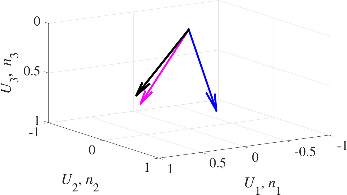 Figure 1
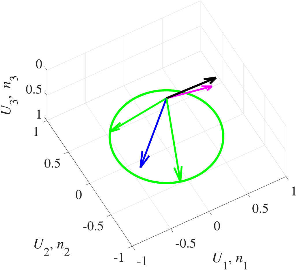 Figure 2
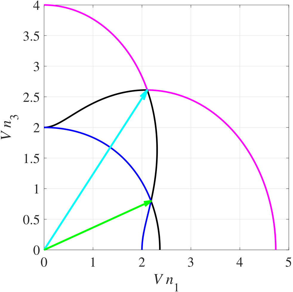 Figure 3
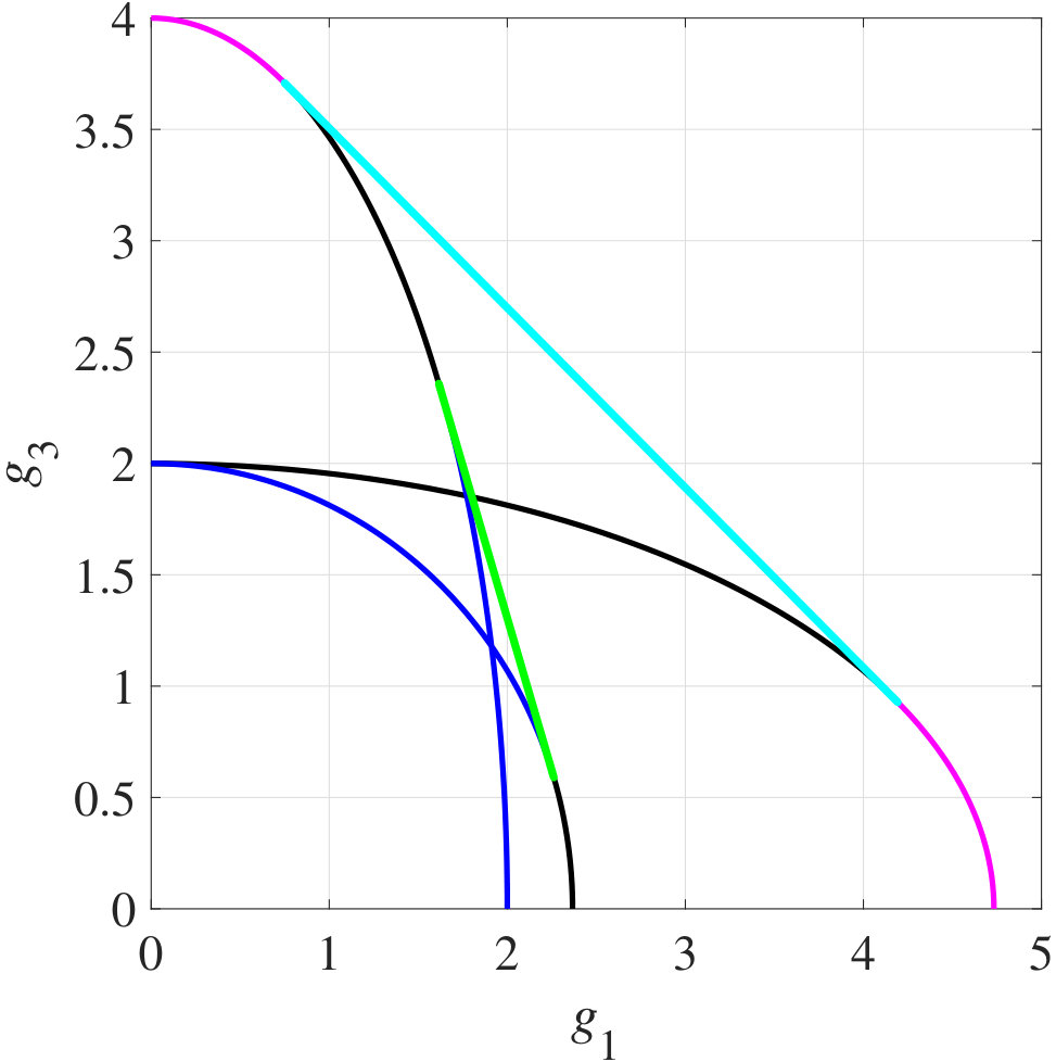 Figure 3
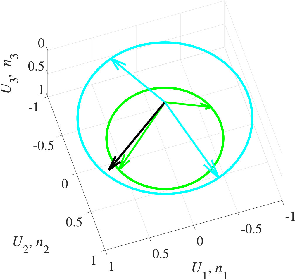 Figure 4
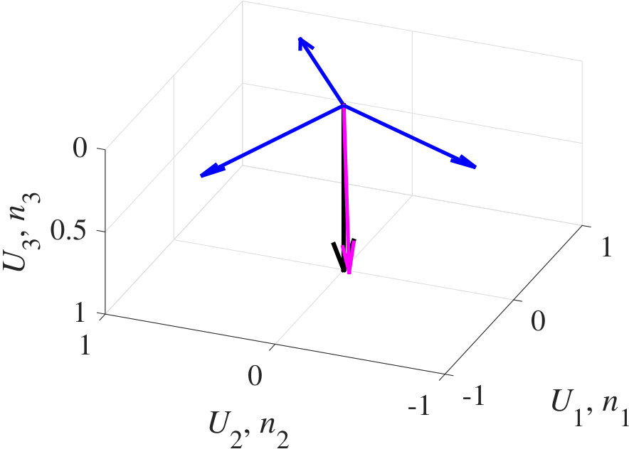 Figure 5
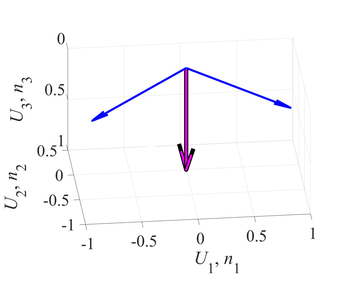 Figure 6
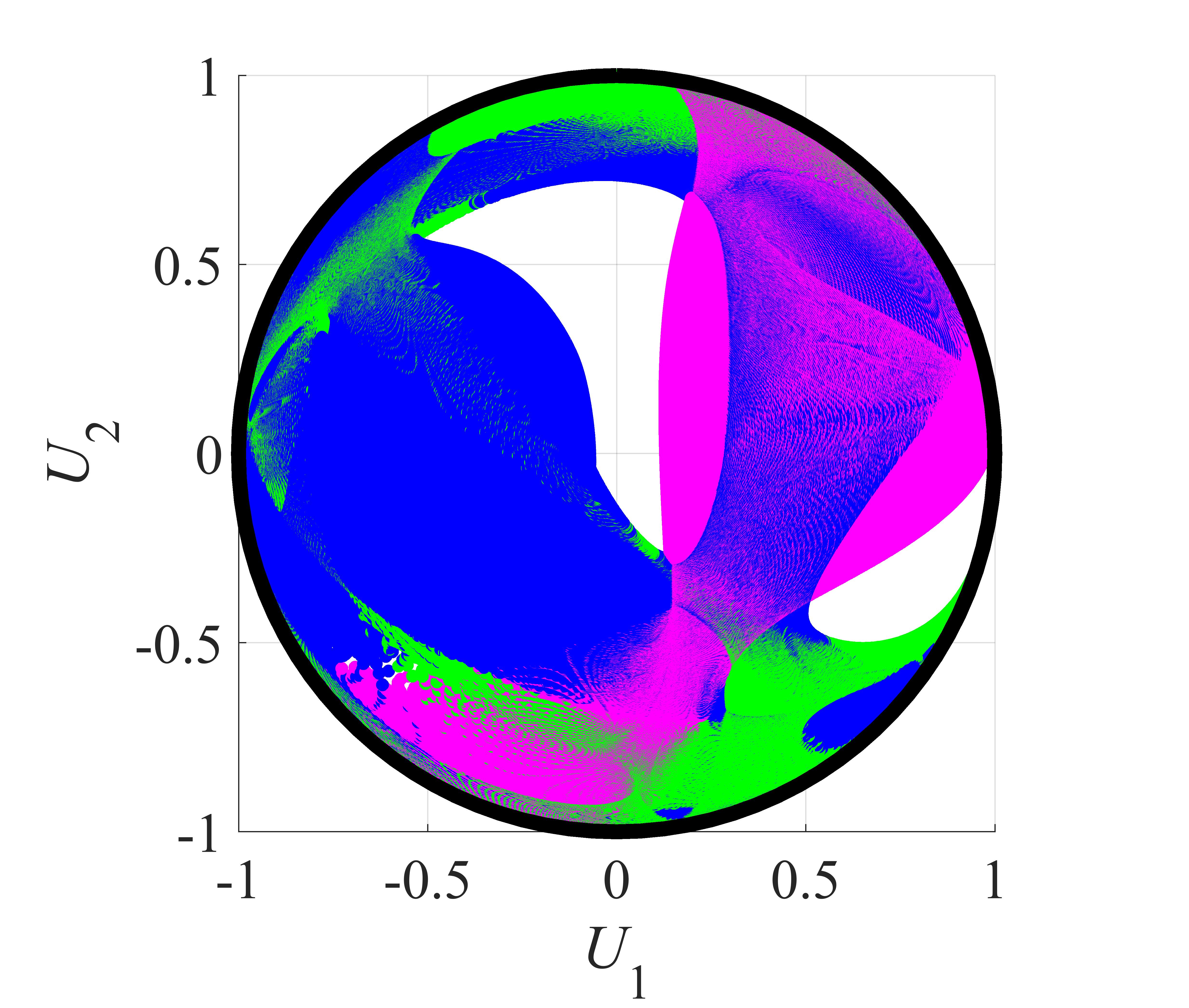 Figure 7
Peer Reviews
No public reviews on file for this paper yet. If you reviewed it on a platform where reviews are public (OpenReview, ICLR, NeurIPS, ICML), you can paste yours below so the community can read it here.
Videos
No videos yet. Explain this paper in a talk, walkthrough, or lecture? Add one.
Christoffel equation in the polarization variables
Vladimir Grechka1
1Borehole Seismic, LLC
Abstract
We formulate the classic Christoffel equation in the polarization variables and solve it for the slowness vectors of plane waves corresponding to a given unit polarization vector. Our analysis shows that, unless the equation degenerates and yields an infinite number of different slowness vectors, the finite nonzero number of its legitimate solutions varies from 1 to 4. Also we find a subset of triclinic solids in which the polarization field can have holes; there exist finite-size solid angles of polarization directions unattainable to any plane wave.
pacs:
81.05.Xj, 91.30.-f
I Introduction
The Christoffel Christoffel (1877) equation governs the propagation of plane waves in homogeneous anisotropic media. A textbook approach (e.g., Fedorov, 1968; Musgrave, 1970; Auld, 1973) to solving it consists in specifying the unit wavefront normal vector , constructing the symmetric, positive-definite Christoffel tensor , and computing solution to the ensuing eigenvalue-eigenvector problem — the phase velocities and the unit polarization vectors of three body waves propagating along the selected wavefront direction . If that is not a singularity, all three vectors are unique; alternatively, if happens to be a singularity, some of vectors or all of them are nonunique.
The introduction of the slowness vector translates the uniqueness of into uniqueness of the corresponding group-velocity vector (e.g., Fedorov, 1968; Musgrave, 1970). Its normalized version, the ray vector , emerges in two-point ray-tracing (e.g., Červený, 2001) as a natural variable for the description of velocities and polarizations of high-frequency waves, their number, for a given ray direction in a homogeneous anisotropic medium, ranging from three to nineteen Grechka (2017). Thus, all properties of plane waves propagating in a homogeneous anisotropic medium can be computed as functions of either unit vector or .
This paper discusses a similar computation for a unit polarization vector selected as such a primary variable. A physical experiment encouraging the understanding of waves parameterized by would be a record of wave motion by a single three-component sensor placed in a homogeneous elastic solid. If such a sensor is located sufficiently far from a source, it would record vectors of individual body waves. Then one might wonder what kind of information about the local velocities or slownesses of these waves could be extracted from the measured direction of and the knowledge of the medium — the inquiry pursued here.
II Theory
An obvious point of departure for our investigation is the Christoffel equation (e.g., Fedorov, 1968; Musgrave, 1970; Auld, 1973)
[TABLE]
where is the slowness vector, is the unit polarization vector,
[TABLE]
is the second-rank positive-definite Christoffel tensor or matrix, and is the fourth-rank density-normalized stiffness tensor. We wish to solve equation 1 for given the knowledge of and .
One can immediately observe that function is not necessarily unique. A simple example, exposing its nonuniqueness, is supplied by SH-waves propagating in the vertical plane of a purely isotropic medium, the waves that have identical polarization vectors for any in-plane slowness vector . Still, the presented exception does not negate the fact that equation 1 is a system of three quadratic equations for the three components of slowness vector . When non-degenerative, system 1 has a finite number of roots, and Bézout’s theorem Weisstein (2003) equates their maximum number to the product of degrees of individual equations, that is, . Also because a real-valued root of system 1 is always accompanied by its centrally symmetric opposite ,
The maximum number of distinct (that is, non-centrally symmetric) real-valued roots of non-degenerative system 1 is equal to 4.
Once these slowness roots are found, the corresponding phase and group velocities are given by Fedorov (1968); Musgrave (1970); Auld (1973)
[TABLE]
and
[TABLE]
III Isotropy
The analysis of system 1, shorthanded as the problem, is easiest in isotropic media, where the system does not even need to be solved to understand the properties of its solutions. Indeed, because for the P-waves and for the S-waves, a given vector uniquely constrains and yields infinitely many slowness vectors , confined to the plane orthogonal to .
Let us derive this simple result from equation 1. Because all directions are equivalent in isotropic media, the coordinate axis can be oriented along our polarization vector that becomes in the new coordinate frame. Then, the substitution of that in system 1, written for isotropic stiffness tensor expressed in terms of Lamé constants and , reduces the system to
[TABLE]
implying two possible scenarios.
1.
If equations 5cb and 5cc are satisfied by setting , equation 5ca yields a uniquely defined direction of the centrally symmetric P-wave slowness vector
[TABLE]
2.
Alternatively, if both equations 5cb and 5cc are satisfied by setting , equation 5ca, relating the two remaining unknowns and , describes a circle in the plane, resulting in the S-wave slowness vectors
[TABLE]
and confirming the fact that the shear-wave slowness vector cannot be uniquely derived from polarization vector .
IV Vertical transverse isotropy
The problem in vertically transversely isotropic (VTI) media offers much more variety than that in just examined isotropic media, entailing several intriguing special cases. We will analyze them as they get discovered, starting from the general scenario, in which all three components of a given polarization vector are nonzero, and system 1 reads Fedorov (1968); Tsvankin (2001)
[TABLE]
where are the density normalized stiffness coefficients in Voigt notation.
Mere inspection of matrix in the left side of system 17 reveals a special case: if (unlikely for natural materials but mathematically possible), one eigenvector of such a is always vertical, whereas two other eigenvectors are always horizontal regardless of the value of . Although superficial reaction to this observation might be that equations 17 become incompatible for an arbitrary direction of , a more careful investigation, presented below, is warranted.
When , as typically expected in VTI solids, matrix has one horizontal eigenvector corresponding to the SH-wave. Hence, unless — another special case — the SH-wave slowness vector cannot be obtained by solving equations 17 for the components of . Consequently, equations 17 can have two real-valued roots that describe slowness vectors of the P- and SV-waves for an arbitrary polarization vector .
Figure 1, computed for a VTI stiffness matrix (in arbitrary units of velocity squared, as well as other stiffness matrixes below)
[TABLE]
with “SYM” denoting the symmetric part of , illustrates this arrangement. Equations 17 have the real-valued slowness solutions and , and Figure 1 displays the corresponding wavefront normals . The P-wave normal (magenta) is close to the polarization vector (black), whereas the SV normal (blue) is approximately orthogonal to it.
The two slowness solutions shown in Figure 1, however, do not exhaust all the possibilities. If a VTI model possesses intersection singularities (in the terminology of Crampin and Yedlin, 1981) , polarization vector at a singularity might happen to be equal to an input vector , making the singular slowness vector a part of real-valued solution of equations 17; also because a vertical plane containing an arbitrary vector is a symmetry plane of a VTI medium, singular solutions of equations 17 always come in non-centrally symmetric pairs.
To investigate this scenario, we increase the stiffness coefficient in matrix 18 to make and create an intersection singularity in VTI model
[TABLE]
at in the plane. Figure 2 presents the obtained wavefront normals for the same polarization vector (the black arrow) as that in Figure 1. Indeed, the two singular wavefront normals (the green arrows in Figure 2) have been recovered from equations 17 in addition to (the magenta arrow) and (the blue arrow).
IV.1 Equality
The presented example allows us to understand how to properly treat the special case of equality
[TABLE]
Even though matrix in system 17 does have one vertical and two horizontal eigenvectors, the presence of intersection singularities could make equations 17 compatible for an arbitrary polarization vector . To illustrate that, let us impose constraint 20 on VTI stiffness matrix 19, so that it becomes
[TABLE]
Model 21 exhibits two intersection singularities and , indicated by the cyan and green arrows in Figure 3a, and two corresponding internal refraction cones, degenerating into the cyan and green straight lines in Figure 3b. The fans of polarization vectors and at those singularities contain vectors equal to the input polarization vector (the black arrow in Figure 4). Hence, all four solutions of equations 17 for this vector come from the intersection singularities.
Finally, let us investigate two symmetric orientations of vector — along the vertical symmetry axis and orthogonally to it.
IV.2 Vertical polarization vector
When input polarization vector is vertical, , system 17 simplifies to
[TABLE]
and becomes very similar to system 5c examined for isotropic media. Consequently, three types of solutions are possible — two already analyzed in section III and one related to the equality , whose analog is prohibited for isotropy by the elastic stability conditions.
1.
When equations 22ca and 22cb are satisfied by setting , equation 22cc yields the vertical P-wave slowness vector
[TABLE]
2.
When equations 22ca and 22cb are satisfied by setting , equation 22cc, relating the two remaining unknowns and , describes infinitely many shear-wave slowness vectors
[TABLE]
their ends tracing a circle with radius in the plane.
3.
Finally, when , equations 22ca and 22cb are satisfied identically for any slowness vector, whereas equation 22cc constraints the components of to the surface of a spheroid in the -space.
IV.3 Horizontal polarization vector
Because all horizontal directions in a VTI medium are equivalent due to its rotational invariance around the vertical, let us select to simplify our analysis. System 17 then reads
[TABLE]
implying three possibilities similar to those just discussed for the vertical vector .
1.
When equations 25cb and 25cc are satisfied for , equation 25ca describes the horizontal P-wave slowness vector
[TABLE]
2.
When both equations 25cb and 25cc are satisfied for , equation 25ca yields infinitely many SH-wave slowness vectors
[TABLE]
their ends placed at an ellipse in the vertical plane.
3.
When and equation 25cb is satisfied for ( in accordance with the elastic stability conditions in VTI media), equation 25ca describes the slowness vectors given by equation 27. Alternatively, when but equation 25cb is satisfied for instead of , equation 25ca describes a set of the slowness vectors in the plane,
[TABLE]
V Symmetries lower than transverse isotropy
The analysis of the problem presented so far reveals that system 1 can have two, four, or infinitely many slowness solutions for a given polarization vector . Clearly, the first two possibilities are realizable in generally anisotropic media because roots of a polynomial system are continuous functions of its coefficients, which are, in turn, continuous functions of the stiffness components. For instance, Figure 5 displays four singularity-unrelated solutions (the magenta and blue arrows) for triclinic model
[TABLE]
The number of real-valued roots of equations 1 in low-symmetry anisotropic media can be infinite, too. Consider, for example, the vertical polarization vector in an orthorhombic solid described by its generic stiffness matrix. There, equations 1 reduce to a system similar to 22c,
[TABLE]
and because equations 30ca and 30cb are simultaneously satisfied at , equation 30cc yields an infinite number of slowness vectors
[TABLE]
Hence, it remains to investigate whether equations 1 can have zero, one, or three real-valued roots. To address the question pertaining to the existence of one or three real-valued roots in a systematic way, we select a local coordinate frame, in which our input polarization vector , and explicitly write system 1 for that in triclinic media. The system reads
[TABLE]
lending itself to straightforward analysis.
V.1 One root
If a triclinic model is such that
[TABLE]
the cross-terms vanish in equation 32ca; if additionally
[TABLE]
the terms proportional to vanish in both equations 32ca or 32cb; finally, if the product
[TABLE]
equations 32ca and 32cb are satisfied for a single pair of real-valued slowness components , and equation 32cc yields a single centrally symmetric slowness root
[TABLE]
V.2 Three roots
Alternatively, if the opposite of inequality 35 is true,
[TABLE]
equation 32ca has two roots, related to each other as
[TABLE]
and complementing the already discussed root . Therefore, system 32c can possess three real-valued roots, as shown in Figure 6 for triclinic stiffness matrix
[TABLE]
The logic presented for equation 32ca would apply to equation 32cb when the set of equalities 33c is replaced by
[TABLE]
and inequalities 35 or 37 are replaced by
[TABLE]
or
[TABLE]
respectively.
VI Prohibited polarization directions
An unexpected scenario arises when equations 33c are satisfied, and the signs of three nonzero stiffness coefficients composing the triplet \big{[}c_{15},\,c_{35},\,c_{46}\big{]} coincide,
[TABLE]
Then equation 32ca, now in the form
[TABLE]
has only trivial real-valued solution
[TABLE]
making system 32c incompatible.
As a result, our polarization direction is unattainable to any plane wave regardless of its wavefront normal ; and the field of polarization vectors develops a hole at the vertical. The size of this hole, outlining a solid angle of prohibited polarization directions, is finite rather than infinitesimal because a small finite perturbation of order of the components of vector replaces equation 44 by
[TABLE]
and solution 45 by a real-valued slowness vector that has the length
[TABLE]
provided that the sign of the right side of equation 46 coincides with that of the stiffnesses in the triplet \big{[}c_{15},\,c_{35},\,c_{46}\big{]}; otherwise, a solution becomes complex-valued. Clearly, the length of vector given by relationship 47 is too small to ensure the compatibility of equations 32c.
To illustrate possible sizes of solid angles of prohibited polarization directions, we construct a triclinic model
[TABLE]
in which the boldface stiffness coefficients obeying conditions 33ca, 33cb, 33cc, and 43ba are typeset in black, blue, red, and green, respectively. Next, we solve the Christoffel equation
[TABLE]
analogous to equation 1, in model 48 for a set of wavefront normals spanning the entire unit sphere. The obtained polarization vectors , displayed in Figure 7, exhibit two finite-size solid angles of prohibited polarization directions, appearing as the white areas.
VII Discussion and conclusions
The presented analysis allows us to list all the possibilities of describing plane-wave propagation in homogeneous anisotropic media in terms of a single input quantity — the unit vector , , or .
1. Input wavefront normal .
Solving the Christoffel equation 49 always yields three phase velocities , , and of the P-, S1-, and S2-waves, equal to square roots of the eigenvalues of Christoffel tensor .
- •
If , the wavefront normal direction is non-singular, and equation 49 results in three distinct eigenvectors — the unit polarization vectors , , and . Then equation 4 defines three group-velocity vectors , , and and three unit ray-direction vectors , , and , the triples of both vectors and uniquely determined.
- •
Alternatively, if at least two phase velocities , , and coincide, the wavefront normal direction becomes singular, , generally resulting in an infinite number of polarization vectors of body waves corresponding to the singularity. Only at kiss singularities (e.g., Crampin and Yedlin, 1981) the uniqueness of vectors and is maintained despite the nonuniqueness of . All other singularities produce an infinite number of vectors and .
2. Input ray direction .
Equations 22 in Grechka Grechka (2017) or equations 2.C.13 and 2.C.14 in Grechka and HeiglGrechka and Heigl (2017) comprise an algebraic system of degree 43 that has an odd number of non-centrally symmetric real-valued solutions \big{\{}\bm{n}(\bm{r}),\,\bm{U}(\bm{r})\big{\}}, ranging from 3 to 19 and representing the uniquely determinable parameters of plane waves propagating along a given ray direction . Although the system degenerates at kiss singularities because of the nonuniqueness of , it yields a unique wavefront normal there.
3. Input polarization vector .
Equations 1 solved for the slowness vector can have from 0 to 4 or infinite number of real-valued solutions and the same number of solutions for the group-velocity vector .
Clearly, different inputs — , , or — lead to very different descriptions of wave propagation in homogeneous anisotropic media. The knowledge of either the wavefront normal or the ray direction guarantees the presence of at least three plane body-wave solutions, whereas the specification of polarization vector can result in no solutions.
The reference list from the paper itself. Each links out to its DOI / PubMed record.
- 1Christoffel (1877) E. B. Christoffel, Annali di Matematica 8 , 193 (1877).
- 2Fedorov (1968) F. I. Fedorov, Theory of elastic waves in crystals (Plenum Press, 1968).
- 3Musgrave (1970) M. J. P. Musgrave, Crystal acoustics (Holden-Day, 1970).
- 4Auld (1973) B. A. Auld, Acoustic fields and waves in solids (John Wiley and Sons., 1973).
- 5Červený (2001) V. Červený, Seismic ray theory (Cambridge University Press, 2001).
- 6Grechka (2017) V. Grechka, Geophysics 82 , no. 4, WA 45 (2017).
- 7Weisstein (2003) E. W. Weisstein, CRC concise encyclopedia of mathematics (Chapman & Hall/CRC, 2003).
- 8Tsvankin (2001) I. Tsvankin, Seismic signatures and analysis of reflection data in anisotropic media (Elsevier, 2001).