Coherent Showers in Decays of Colored Resonances
Helen Brooks, Peter Skands

TL;DR
This paper introduces a new coherent parton shower model for decays of colored resonances using resonance-final antennae, improving the accuracy of simulations in high-energy physics, especially for top quark production.
Contribution
It develops a novel RF antenna-based formalism for coherent showers, implemented in PYTHIA 8, and applies it to top quark production at the LHC with NLO matching.
Findings
The new shower respects QCD coherence and reduces to known kernels in limits.
Implementation in PYTHIA 8 with NLO matching shows promising results.
Recommendations for theoretical uncertainty assessment are provided.
Abstract
We present a new approach to coherent parton showers in the decays of coloured resonances, based on the notion of "resonance-final" (RF) QCD antennae. A full set of mass- and helicity-dependent antenna functions are defined, with the additional requirement of positivity over the respective branching phase spaces. Their singularity structure is identical to that of initial-final (IF) antennae in hard processes (once mass terms associated with the incoming legs are allowed for), but the phase-space factorisations are different. The consequent radiation patterns respect QCD coherence (at leading colour) and reduce to Dokshitzer-Gribov-Lipatov-Altarelli-Parisi and eikonal kernels in the respective collinear and soft limits. The main novelty in the phase-space factorisation is that branchings in RF antennae impart a collective recoil to the other partons within the same…
Click any figure to enlarge with its caption.
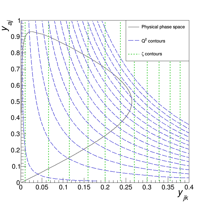 Figure 1
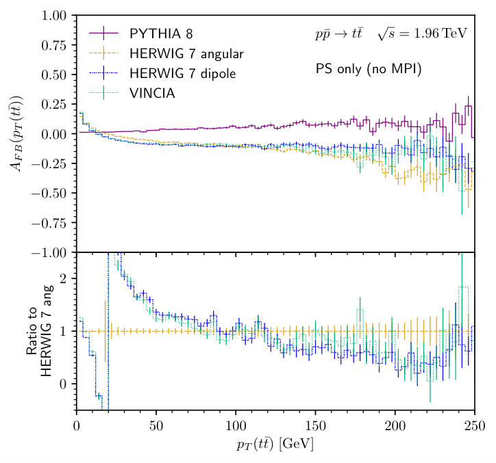 Figure 2
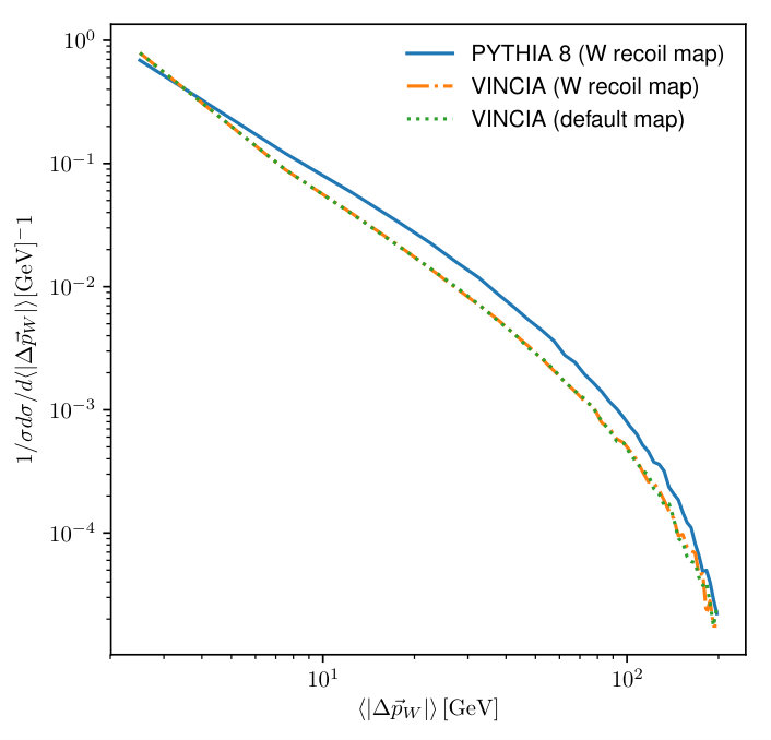 Figure 3
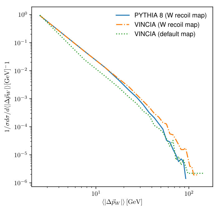 Figure 4
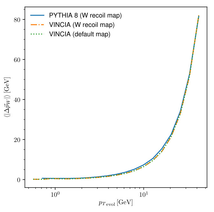 Figure 5
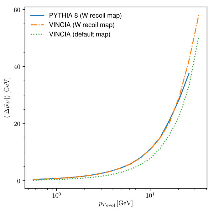 Figure 6
 Figure 7
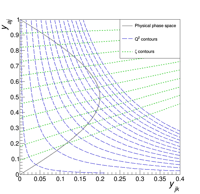 Figure 8
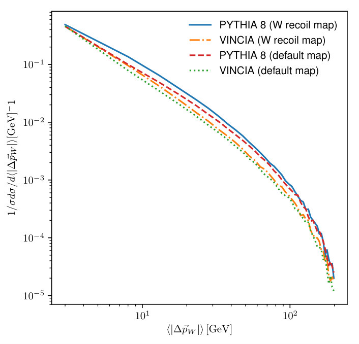 Figure 9
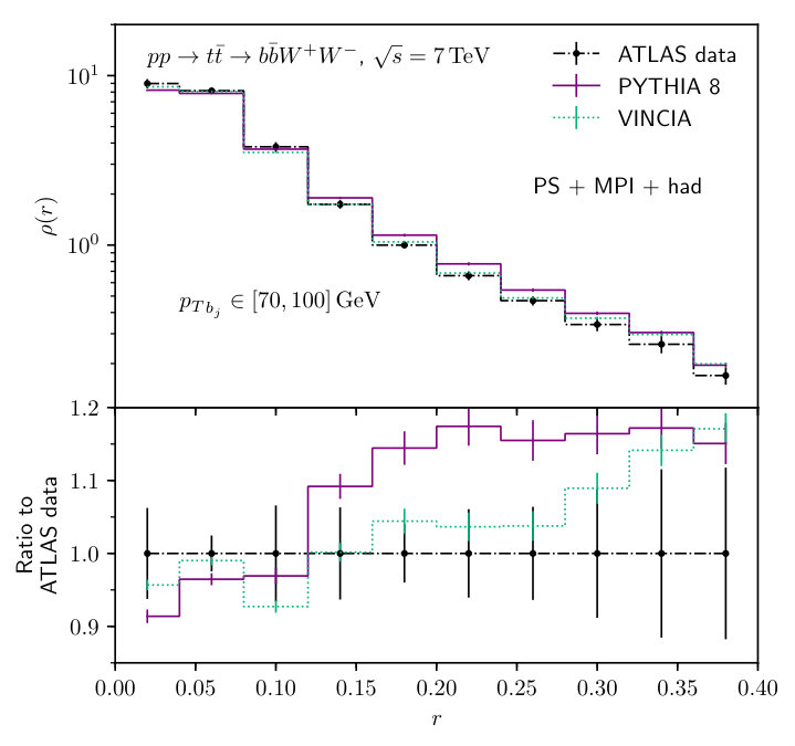 Figure 10
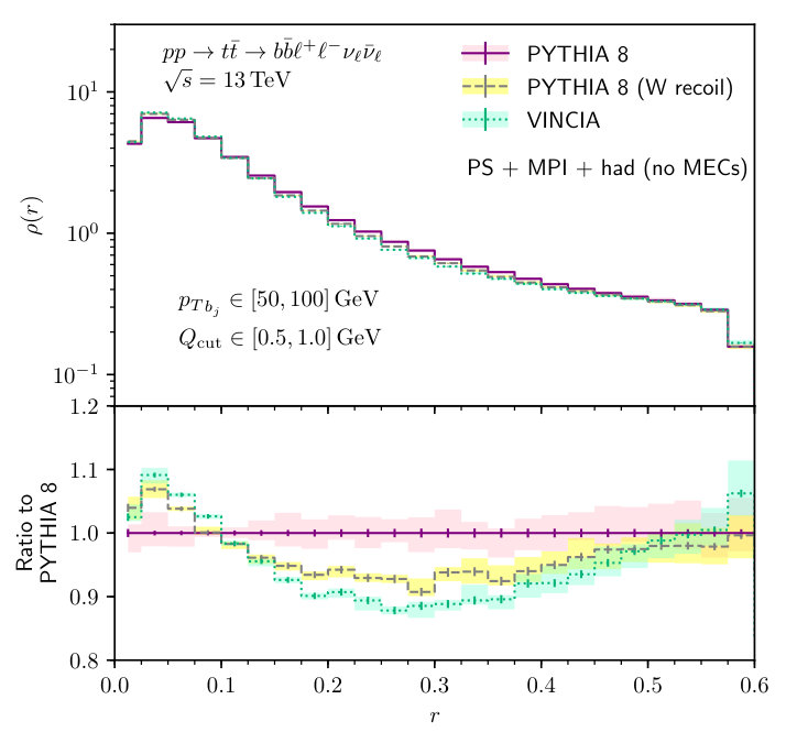 Figure 11
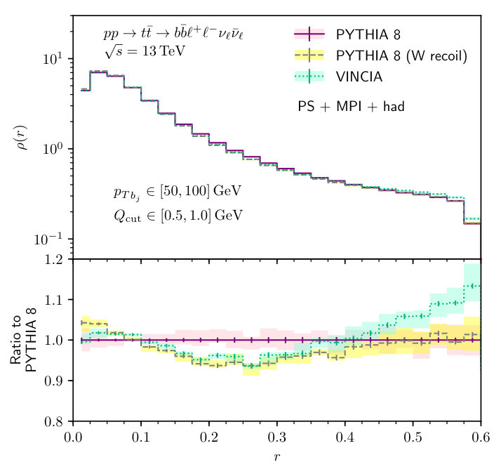 Figure 12
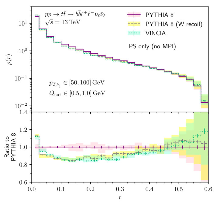 Figure 13
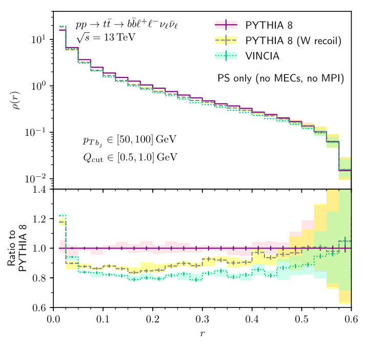 Figure 14
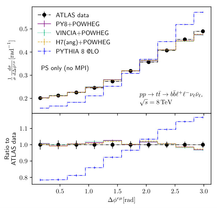 Figure 15
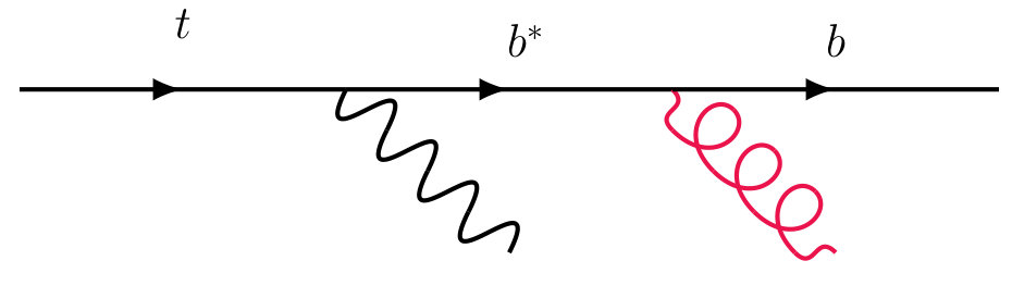 Figure 16
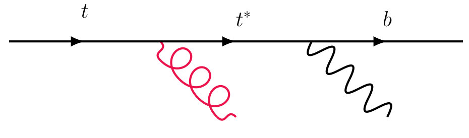 Figure 17
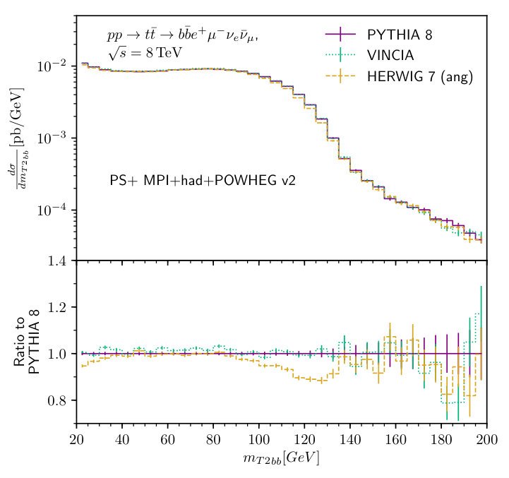 Figure 18
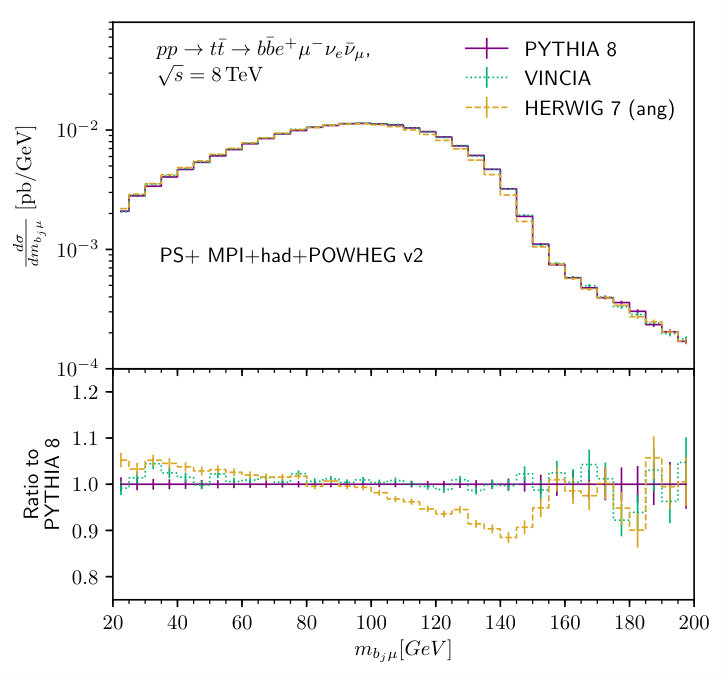 Figure 19
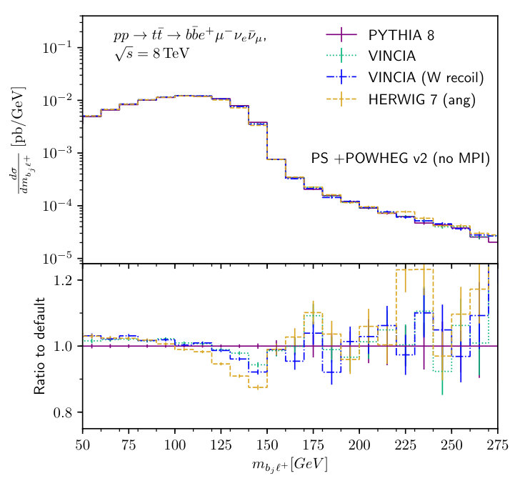 Figure 20
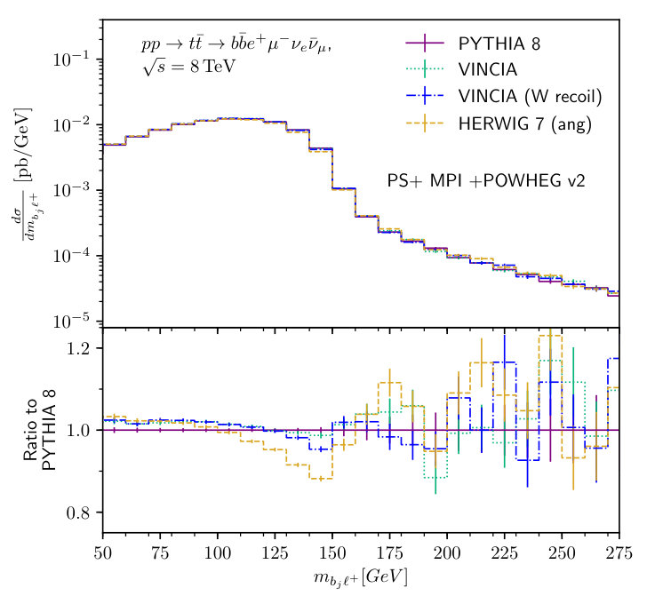 Figure 21
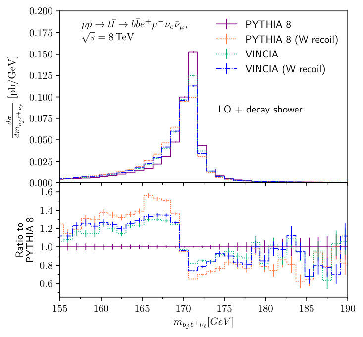 Figure 22
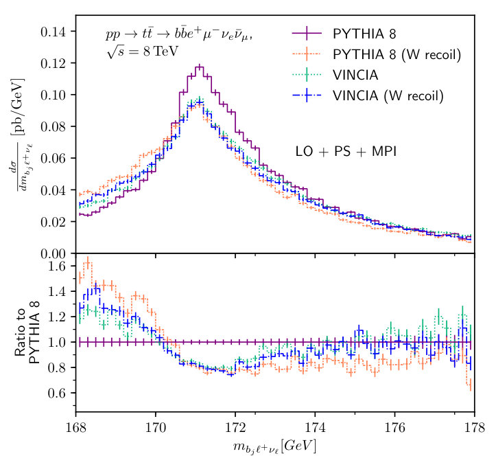 Figure 23
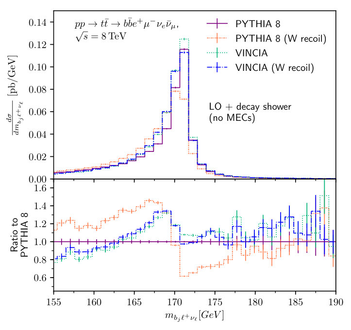 Figure 24
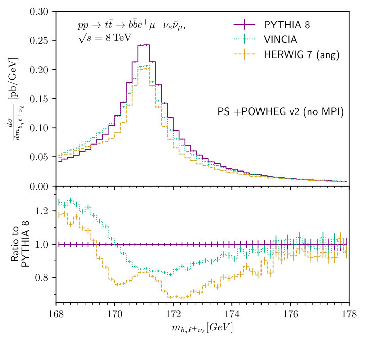 Figure 25
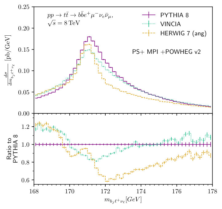 Figure 26
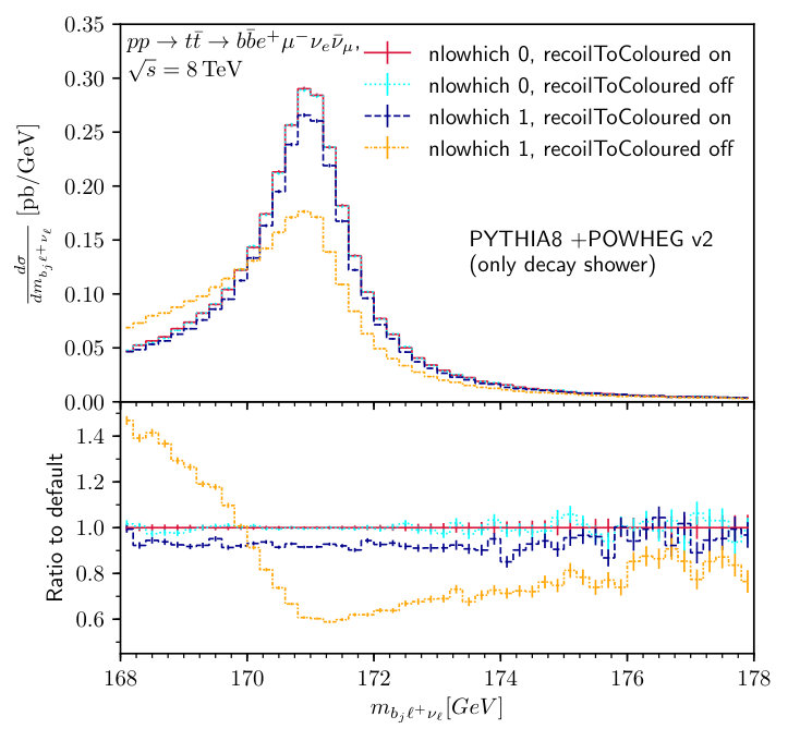 Figure 27
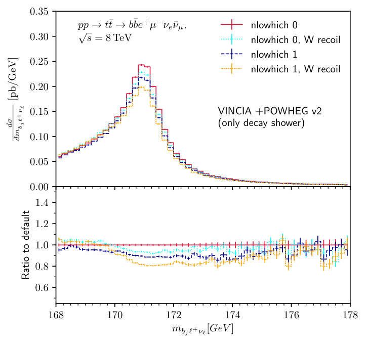 Figure 28
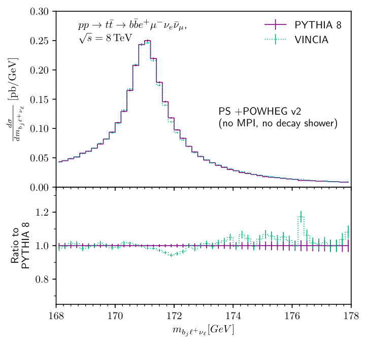 Figure 29
 Figure 30
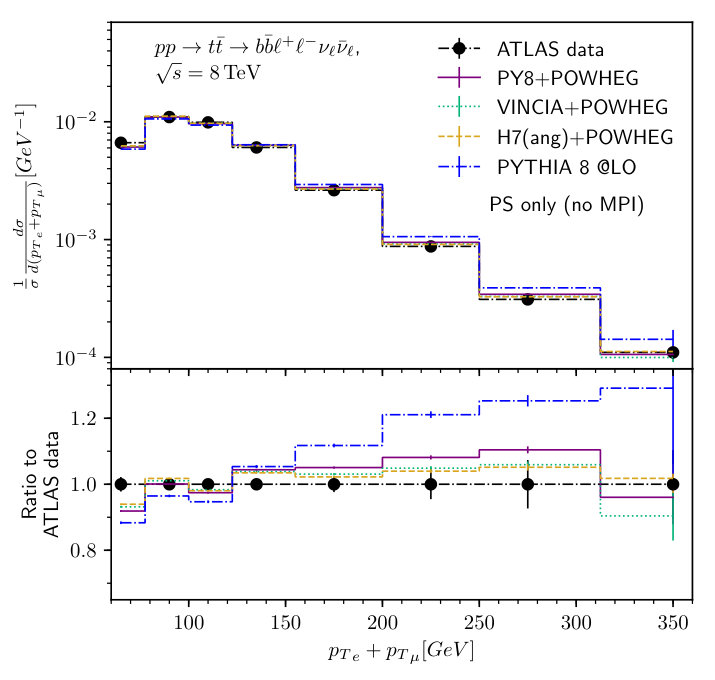 Figure 31
 Figure 32
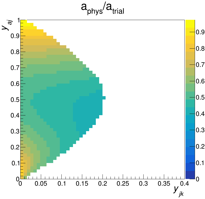 Figure 33
 Figure 34
 Figure 35
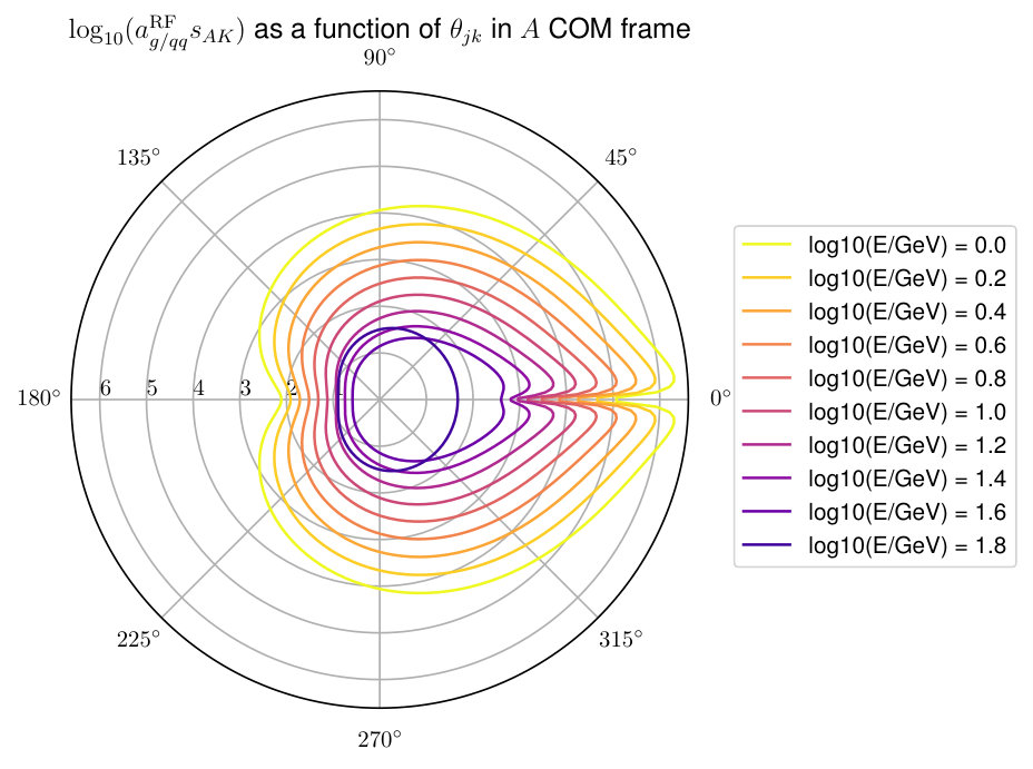 Figure 36
Peer Reviews
No public reviews on file for this paper yet. If you reviewed it on a platform where reviews are public (OpenReview, ICLR, NeurIPS, ICML), you can paste yours below so the community can read it here.
Videos
No videos yet. Explain this paper in a talk, walkthrough, or lecture? Add one.
Coherent Showers in Decays of Coloured Resonances
Helen Brooks
Peter Skands
School of Physics and Astronomy, Monash University
Wellington Road, Clayton, VIC-3800, Australia
Abstract
We present a new approach to coherent parton showers in the decays of coloured resonances, based on the notion of “resonance-final” (RF) QCD antennae. A full set of mass- and helicity-dependent antenna functions are defined, with the additional requirement of positivity over the respective branching phase spaces. Their singularity structure is identical to that of initial-final (IF) antennae in hard processes (once mass terms associated with the incoming legs are allowed for), but the phase-space factorisations are different. The consequent radiation patterns respect QCD coherence (at leading colour) and reduce to Dokshitzer-Gribov-Lipatov-Altarelli-Parisi and eikonal kernels in the respective collinear and soft limits. The main novelty in the phase-space factorisation is that branchings in RF antennae impart a collective recoil to the other partons within the same decay system. An explicit implementation of these ideas, based on the Sudakov veto algorithm, is provided in the Vincia antenna-shower plug-in to the Pythia 8 Monte Carlo event generator. We apply our formalism, matched to next-to-leading order accuracy using Powheg , to top quark production at the LHC, and investigate implications for direct measurement of the top quark mass. Finally, we make recommendations for assessing theoretical uncertainties arising from parton showers in this context.
††preprint: MCNET-19-15
I Introduction
In the reconstruction of resonances produced at the Large Hadron Collider, Shower Monte Carlo (MC) event generators (see [1]) play an ongoing critical role. Despite this, many are only formally accurate to leading-logarithm, such that there remains a range of ambiguities in their precise definition, for example, in the exact form of the splitting kernels used to define emission probabilities and Sudakov factors. This in some cases can lead to large theoretical uncertainties in direct measurements, of which the most notable example is the mass of the top quark. Nevertheless, analogous to the notion of using “sensible” scale choices for evaluating matrix elements of hard processes, some ambiguities can be guided by the inclusion of well-motivated physical properties. One such formally subleading property is that of coherence.
In kinematic limits that correspond to approximately on-shell internal propagators, quantum field theory amplitudes exhibit simple and universal factorisation properties. These are at the heart of both the treatment of (sequential) resonance decays and bremsstrahlung corrections in high-energy processes. Decay processes in the narrow-width limit, as well as the collinear limits of bremsstrahlung processes, are particularly simple (modulo spin correlations), and can be obtained from (squared) Feynman amplitudes which each involve only a single divergent propagator structure. The soft limits, however, characterised by so-called eikonal factors, intrinsically involve a coherent sum over several interfering amplitudes, each with a different propagator structure.
In QCD, one starts from the leading-colour (LC) approximation, which reduces the number of interfering amplitudes that need to be considered to just two for a given gluon becoming soft in a given colour ordering. These are the two amplitudes that contribute to the corresponding eikonal factor. For the specific case of decays of coloured resonances, the radiation patterns are normally cast solely in terms of emissions from the produced decay products. The reasoning for this is that in the rest frame of the decaying particle the contribution to the radiation patterns from the decaying resonance itself can be neglected, and that the distinction between which particle radiates is anyway gauge dependent and hence unphysical. Formally, one may partition the full (coherent and gauge invariant) radiation pattern into a term representing radiation from the decaying resonance and one representing radiation from its decay product(s). This is illustrated for top decay in fig. LABEL:fig:feynTB.
The former is subdominant (depending on the details of the partitioning, it may even turn out to be negative) and is neglected in most current Shower MC implementations we are aware of. It is worth emphasising that matrix-element corrections (MECs) are widely used (e.g., in Pythia and in Powheg) to correct the first emission to the full result; but in this work we wish to address the issue of coherence in resonance decays more generally, and apply it to all emissions.
Noting that the antenna-shower formalism (see [2, 3, 4]) does not require a partitioning of the radiation pattern into “radiators” and “spectators”, we derive a set of coherent antenna functions for “resonance-final” (RF) colour flows, with full mass- and helicity-dependence. We note that these functions exhibit the same singularity structures as corresponding “initial-final” (IF) antenna functions derived elsewhere [4, 5], once general mass terms are allowed for in the latter. Somewhat arbitrarily we also choose the nonsingular terms to be the same for the IF and RF antenna functions, with minor changes relative to [4, 5] to ensure that all of the IF and RF antenna functions remain positive over all of their respective phase spaces. This makes them straightforward to interpret in the probabilistic context of a Shower MC. We combine these antenna functions with a recoil strategy (alternatively known as a “kinematics map”) which preserves the 4-momentum of the decaying resonance (and hence in particular its invariant mass), while imparting a (collective) recoil to the other final-state particle(s) produced in the decay. We argue that this approach should exhibit improved coherence properties over the baseline Pythia shower model [6, 7], and that it represents an interesting alternative to other current Shower MC implementations. We also show that it combines quite naturally with resonance-aware matching in the Powheg formalism [8, 9, 10, 11, 12].
Finally, we consider top quark production as a case study for an application of our formalism. This is a particularly well-motivated example, since it was recently noted in [13, 14] that the existing approaches of Pythia 8.2 [15, 6, 16, 17] and Herwig 7.1 [18, 19, 20, 21, 22] exhibit substantial shape differences in their predictions for the differential distribution of the reconstructed invariant mass of the top, already at the level of the parton shower. This has potential implications for the minimum uncertainty present in the measurement of the top quark pole mass extracted through direct methods. Reducing this uncertainty is desirable since not only is the top quark mass an important parameter for many Beyond-the-Standard-Model extensions, but also since the stability of the electroweak vacuum is highly sensitive to its precise value [23].
The outline of the paper is as follows. In section II we give a review of existing treatments of resonance decays in Shower MCs. In section III we provide details of our new implementation of resonance decays within the Vincia antenna shower. In section IV we describe resonance-aware matching methods in Powheg, and how these may be used alongside Vincia. In section V we present our results for top quark production. Finally, we summarise in section VI.
II Review of Existing Treatments of Resonance Decays
There are already a range of existing frameworks available for the treatment of resonance decays, so before describing our implementation we briefly review these alternatives.
There are a number of components to a parton shower in which there is some flexibility, that must be defined for the shower to be fully specified. These include the precise form of the splitting kernels in no-emission probabilities, the recoil strategy employed, and the nature of the evolution variables used (which determine how ordered sequences of emissions are generated). One manner of classifying the available options is via the method chosen for organising the singular limits across the set of functions that represent the underlying colour-connected objects (each of which is deemed to radiate independently in the leading-colour approximation). As already noted, in the global antenna-dipole shower framework [24, 2, 25, 26, 3, 4], a single antenna function contains the entire soft singularity of two colour-connected partons, but the collinear limit for gluons is partitioned across two neighbouring antennae. In the “partitioned-dipole” class of showers, both collinear and soft singularities are partitioned across neighbouring dipoles, and in the case of initial-final colour flows, one distinguishes between separate final-initial and initial-final dipole ends (the sum of which is equivalent to a single initial-final antenna in the antenna-shower framework). Of this type there are two main variants.
The first is based on Catani-Seymour factorisation, and the form of the splitting kernels are those used in the Catani-Seymour dipole subtraction method [27, 28, 29]. Such a shower is the default used in the Sherpa event generator [30], and more recently is also available as an option in Herwig 7 [31, 20, 21]. Here the eikonal is carefully partitioned such that coherence should be recovered after summing over all dipoles. While this procedure is effective for massless initial state particles, since mass corrections are typically negative, the initial-final dipole end in resonance decays can become negative. Sherpa and Herwig offer slightly different solutions to this issue. In Sherpa [32], the resonance is taken to not radiate in decay; instead the entire singularity structure is given to the coloured particle in decay, in a manner akin to a sector antenna shower [33]. All recoil is given to the uncoloured final-state decay product (e.g. in the always takes the recoil.) In the Herwig dipole shower [22] the contribution from the initial-final dipole end is neglected entirely; the recoil from the final-initial dipole end is shared out between all the other decay products present (this is a similar approach to our implementation, described in section III.1). We note that currently the dipole shower option for Herwig is only available for strictly on-shell resonances.
Another variant of the partitioned-dipole shower is the transverse-momentum-ordered shower implemented in Pythia 8 [6, 16, 7, 17]. Here, although the individual soft limits for each radiator are reproduced with the vanishing of the ordering variable, it is known that the partition across initial-final dipoles does not preserve coherence [34]. Despite the lack of coherence, this can be corrected to some extent through matrix-element corrections [15], which is the default option. In addition, ordering in transverse momentum allows for sufficiently compatible definitions such that the multiple-parton interactions (MPI) can be interleaved with the primary parton shower [6, 7]. Pythia 8 has two options for how recoils are performed in resonance decays. The default option is that after the first emission the nearest coloured parton becomes the recoiler. Alternatively it is possible to modify this behaviour so that the original uncoloured decay product always take the recoil (as in Sherpa).
As representative of the class of partitioned-dipole shower we use Pythia 8.240 [17] for later comparisons in section V, in part because there is already available an interface to recent versions of Powheg Box [10, 12, 13]. In addition since both Vincia and Pythia share the same modelling of non-perturbative physics such as hadronisation and underlying event (although they may differ in the default tuned values of parameters controlling these processes), this better allows us to isolate differences that are of perturbative origin.
An alternative to partitioning the singular limits is for each splitting function to take the full singularity structure, and to avoid overcounting via a phase space veto. In this class coherence is guaranteed, since through the phase space veto each emitter can no longer be considered independent. This is the method employed by both sector antenna-showers [33], in the virtuality-ordered shower in Pythia 6 [16], and in traditional angular-ordered showers of which the -shower implemented in Herwig 7 is an example [18]. In the latter, the relative opening-angle between colour-connected partons is imposed as an ordering variable, and must reduce with each subsequent emission. A down-side to angular-ordering is that the phase space factorisation is only approximate, resulting in dead zones away from the singular limits. The -shower was extended to include resonance decays in [22]. As for Sherpa, the uncoloured decay product is again chosen as the recoiler. We take the -shower using Herwig 7.1.4 as representative of this class for later comparisons. Again, this is partially motivated by the presence of an existing interface to Powheg Box [13, 14].
III Antenna Showers in Resonance Decays
III.1 Resonance-Final Phase Space Factorisation
Denoting a generic shower evolution variable by , the no-emission probability for an antenna evolved over the interval is given by the antenna Sudakov factor, , where
[TABLE]
Here is the (3-dimensional) antenna phase space, is a colour- and coupling-stripped antenna function, and is the appropriate colour factor (for a discussion on the conventions used, see [35]). The antenna function captures the leading singularities of the relevant tree-level matrix elements (but may also contain finite terms in addition).
The antenna phase space depends on a factorisation of the post-branching Lorentz invariant phase space,
[TABLE]
in such way that the degrees of freedom of the branching itself and the pre-branching particles can be treated independently. Unlike in traditional parton showers where such phase space factorisations only hold in the soft and collinear limits, eq. 2 is exact.
We now consider the decay of a coloured resonance , where is a final-state particle colour-connected to , and schematically denotes any other decay products. (For example, in , the top quark would be identified with , the quark with , and the with .) The phase space measure is simply [36]:
[TABLE]
where is the Källén function, and , and . There are only two degrees of freedom, representing the global orientation of the frame.
After a branching from the dipole stretching between , we denote the post-branching partons by , where the prime on emphasises that an overall recoil may be imparted to the system. Defining the invariant (as opposed to the , the phase space can be written as:
[TABLE]
where corresponds to a rotation of the branching plane about the original orientation of .
The antenna phase space measure is therefore:
[TABLE]
Implicit in the above derivation is the assumption that the mass of the system of recoilers, is preserved, hence , and that this is equivalent to the antenna mass. In addition we impose that the invariant mass of the resonance is unchanged (a feature that is essential for resonance-aware matching), leading to the identity
[TABLE]
Finally it is presumed that and are produced on-shell.
We now turn to the subject of how the post-branching kinematics are constructed from a given point specified by , , and , subject to the aforementioned constraints. Such a prescription is called a recoil strategy or kinematic map. It is easiest to set up the kinematics in the resonance centre-of-mass frame, such that
[TABLE]
At this stage there remains an ambiguity regarding rotations in the branching plane (about an axis perpendicular to the dipole axis). We specify that only recoils longitudinally with respect to the dipole axis, and all transverse recoil is shared between and . Finally we rotate by about the dipole axis.
Following the above construction, we boost back to the lab frame to recover the momentum of the resonance . Each particle in the system receives its share of the momentum by boosting each by .
We remark that the kinematic map described here is very similar to the prescription recently implemented in [22].
Before concluding this section, we note that had we instead selected a single particle to act as a recoiler, it no longer holds that the mass of the antenna is equivalent to the mass of the recoiler (after the first emission). Supposing we represent the decay as and before and after the emission, and by definition neither nor recoil, factorisation implies we must preserve . Now we also have that
[TABLE]
Thus it becomes impossible to simultaneously preserve and without violating the factorisation. It is undesirable to change either; for example in the case of top decays, where a is selected as the recoiler, the mass should be distributed according to a Breit-Wigner that is very precisely measured, so it would be inappropriate to give it a large virtuality. On the other hand, sacrificing is tantamount to modifying the factorisation eq. 5: everywhere we must replace and . In addition to modifying the volume of phase space, the identity of the invariants is modified with respect to those which appear in the singular part of the real emission matrix elements. Thus a map in which a single particle recoils is pathological from the perspective of the antenna formalism. Nevertheless we have implemented such a map for the sake of understanding its effect, and for more equivalent comparisons with Pythia.
III.2 Massive Initial-Final Antenna Functions
The final-final antenna functions used in Vincia were first derived in [35] and extended to include mass effects in [37]. Massless initial-final and initial-initial antenna functions were presented in [38]. Finally helicity antennae were added in [5] for the massless case.
Here we shall define so-called “resonance-final” antennae where both initial- and final-state partons may be massive. These shall be expressed in terms of the dimensionless invariants, defined as follows:
[TABLE]
The mass corrections act to regulate the collinear limit; furthermore they contribute quite large negative corrections away from the limit. In fact, if only the leading singular terms are retained (for example, the Altarelli-Parisi splitting kernels) these can become negative. However, by including additional finite terms (that are required to vanish in the soft and collinear limits) we can guarantee positive-definiteness over the entire physical phase space.
The full list of helicity-dependent antenna functions may be found in appendix A. Their singular terms are obtained from the massive helicity-dependent final-state antennae through crossing symmetry, while their nonsingular terms have been modified to ensure positivity over the full RF and IF branching phase spaces.
The singular parts of the unpolarised antenna functions (defined as the sum of helicity-dependent antennae, averaging over initial helicities) relevant for top quark decay are, for :
[TABLE]
for :
[TABLE]
where parameterises the partitioning of the collinear singularity of the final-state gluons111Note that the singular part of the term proportional to is antisymmetric under interchange of the two final-state gluons, , hence it cancels when summing over two neighbouring antennae. The default choice is and may be set with Vincia:octetPartitioning, and for splittings of the final-state gluon, :
[TABLE]
Both of the two emission antennae reduce to the (massive) eikonal in the soft () limit:
[TABLE]
These also reproduce the appropriate Altarelli-Parisi splitting functions in the (quasi-)collinear limit [39, 40]:
In addition to being used for coherent branchings in decays of resonances, the same antennae are used for backwards evolution of the initial state, and are then labelled IF antennae; in this case the initial-state partons are restricted to be massless. This choice is to allow consistency with the five-flavour massless scheme, since massive initial partons require corrections to the PDFs222We note, however, that we could in principle use the above antennae also for massive initial state partons, should a set of massive PDFs become available, see e.g. recent developments in [41, 42]..
As mentioned above, we choose (helicity-dependent) nonsingular terms to ensure positivity of all of the antenna functions over both the RF and IF phase spaces. At the unpolarised level, these sum to:
[TABLE]
[TABLE]
and .
In addition to the above “resonance-final” antennae, the following additional initial-final antennae are required to study resonance processes in hadron colliders (for example . For gluon emissions we have:
[TABLE]
and for we have:
[TABLE]
All other antennae may be found in [38, 5].
III.3 Evolution variables
Having demonstrated the desired factorisation we may construct an ordering variable and complementary splitting variable through a change of variables from , . It is worth remarking that there is relative freedom in the choice for these variables: all that is required of is that it vanishes in the soft and collinear limits. The choice for must be linearly independent of and curves of constant should intersect those of constant once and only once. While different choices of should all produce the same result in the soft-collinear limits, they will give rise to subleading differences, which in some cases can be quite significant. For a more in-depth discussion on this point we refer the reader to [35]. Since we take the Jacobian associated with the transformation from () to () explicitly into account, the choice of variable only affects the efficiency of the phase-space sampling and not the final physical distributions.
In the context of interleaved showers [16] it is desirable for the different shower components (e.g., RF and FF antennae for resonance decays, and II, IF, and FF antennae for hard processes) to use similar ordering variables, so that the common sequence of decreasing values of the ordering variables is physically meaningful as a globally decreasing resolution scale. After the first emission in the decay of a resonance, emissions from the RF antenna will compete with emissions from FF antennae in the same decay system. Our choice must therefore be consistent with Vincia’s -ordering variable for FF antennae, which is the same as that used in Ariadne [2, 43],
[TABLE]
For the case of gluon emissions we take:
[TABLE]
while for gluon splittings (to quarks with mass ) we have:
[TABLE]
There is no requirement upon the choices for to be equivalent; therefore convenient choices are selected that are simple, and that allow for the definition of a separable trial integral (as we discuss later in section III.4). We therefore choose:
[TABLE]
for emissions, and
[TABLE]
for splittings.
In fig. 2 we plot contours of constant of and in the , plane.
III.4 Trial Integral
In the context of the Sudakov veto method [16], we generate trial branchings by solving
[TABLE]
for given some random number . Here is the trial integral, obtained by evaluating eq. 1 for some trial antenna function , over a phase space volume equal to or greater than the physical phase space.
The trial antennae must be an overestimate to the physical antenna functions given in section III.2 at every point in phase space; namely they must capture the leading singular behaviour. They must also be simple enough such that both eq. 26 and its inverse are analytically calculable.
Starting with emissions, the change of variables is given by
[TABLE]
For the trial antenna integral, we take:
[TABLE]
This choice captures the leading double soft singularity; in fig. 3(a) we demonstrate numerically that it is a suitable overestimate everywhere in phase space.
Putting everything together we get the following expression for the trial integral:
[TABLE]
where we note that we have averaged over the azimuthal angle , and the integral over is given by:
[TABLE]
The trial integral for depends upon whether fixed or one-loop running of is used333Even if two-loop running of is desired, one-loop running is performed for the trial integral using the 2-loop value of ; this overestimates the two-loop running result and is corrected by including the ratio of in the accept probability., but in either case this is straightforward to perform and invert. Having generated a trial we generate by inverting
[TABLE]
to give
[TABLE]
where is the Lambert W function that is the inverse to (which we implemented according to the method in [44]).
Moving onto splittings, the change of variables is now:
[TABLE]
where is a dimensionless factor given by
[TABLE]
which exhibits the property of being everywhere positive, and tends to unity in the collinear limit (as may be seen in fig. 3(b)). A suitable choice for the trial antenna is therefore
[TABLE]
which captures the leading collinear singularity and exceeds the physical antenna function everywhere in phase space. This is demonstrated numerically in fig. 3(c).
The trial integral is now given by
[TABLE]
and is sampled flatly:
[TABLE]
IV Resonance-Aware Matching with POWHEG
In order to seriously assess theoretical uncertainties, for example in the context of direct top mass measurements at the LHC [45, 46, 47, 48, 49, 50, 51, 52, 53], it is clearly desirable to attain the highest combined logarithmic and fixed-order accuracy that is currently available for the production of resonances.
The matching of parton showers to next-to-leading order accuracy through both subtractive (e.g. MC@NLO) [54] and multiplicative (e.g. Powheg) [8, 9] methods for massive final states has been available for some time [55, 56, 57]. For an accurate reconstruction of resonances however, it is important to correct not only the hardest emission in production, but also in the decay of the resonance. It was noted in [10] that a naive application of the Powheg method to decays (for example as attempted in [58]) in which the kinematics map between the real-emission and the Born phase spaces that modified the virtuality of the resonance, would certainly fail. This conclusion comes from the realisation that differences in the virtuality of the resonance between the and kinematics that exceed its width, spoil the cancellation between the the virtual and real-emission contributions to the cross section. Thus the reweighting of the Born cross section could become arbitrarily large, leading to considerable distortion of the resonance peak. Such difficulties were also expected to be present for subtractive matching methods, as these too could modify the invariant mass of the resonance.
To resolve these issues, a so-called “resonance-aware” matching method was proposed and implemented in Powheg Box v2 [10]. This method performs the next-to-leading-order (NLO) calculation in the narrow width approximation, but applies finite-width effects in an approximate way. Essentially this involves generating fully off-shell resonances for the Born phase space, and mapping to an on-shell phase space to perform the Powheg generation of real emissions, before finally mapping onto the real emission phase space to recover the original resonances’ virtualities. The events are then reweighted to reproduce the correct off-shell next-to-leading-order cross section. In addition this method also includes spin correlations to NLO accuracy. As alluded to earlier, an essential requirement for consistency with the NLO calculation is that the parton shower must preserve the invariant mass of the resonance.
Recently the resonance-aware matching method was extended to include exact width effects [11], before being automated in the generator Powheg Res and applied to the process (bb4l) in [12]. In this method, one must specify the resonance from which a given emission originates. This is straightforward provided there is a single resonance chain, but is not normally possible where there are interfering resonant diagrams. Nevertheless such topologies must be considered in order to extend to exact width effects, as they are technically necessary to preserve gauge invariance. Thus a modification was required to perform the assignment of an emission to a given resonance. The solution was the selection of a given “resonance history” based on a partition of the singular regions of phase space.
In [13] a comparison of the two resonance-aware matching methods and the much earlier hvq implementation for observables relevant to the top mass measurement was performed, using interfaces to Pythia 8.2 and the angular-ordered -shower in Herwig 7.1. It was generally observed that the differences between these two showers for a given method much exceeded the differences resulting from the different choices for the matching method. In the following section where we consider similar observables, we therefore choose to use Powheg Box v2 rather than the more recent generator, as the former is notably faster and we do not expect interference effects to affect our conclusions. We use the setting
allrad = 1
such that emissions are always generated in both the decay and production of the resonance. (This is in addition to the default setting,
nlowhich = 0
which controls whether or not emissions are generated in decay at all.)
Where comparisons to Pythia 8.2 are Herwig 7.1 performed we closely follow the prescription in [13]. For matching to Vincia, the procedure we use is very similar to that used for Pythia. It is necessary to ensure that Vincia does not perform an emission harder than the scale of the emission generated by Powheg. For emissions in production this information is provided via the scalup value in the Les Houches event file, so this must be used as the starting scale in the shower. While for Pythia this behaviour is activated through the settings
TimeShower:pTmaxMatch = 1
SpaceShower:pTmaxMatch = 1
in Vincia, the corresponding setting is :
Vincia:QmaxMatch = 1
In addition, the UserHooks class provided as part of the bb4l package, that is employed for the vetoing of radiation in resonance decays in Pythia, (this being flexible enough also for use with ttbardec in Powheg Box v2) was modified for use with Vincia. The algorithm therein is essentially the same, except for minor modifications for interpreting the event record.
V Applications to Top Quark Physics
V.1 Validation of kinematic map
We shall here validate the kinematic map described in section III.1. We consider the process at a hypothetical collider with TeV. As a measure of the impact of the kinematic map we consider the difference in the three-momentum of the boson, , before and after the first and second emissions from resonance decay system. For Vincia we compare our default map, where the recoil is shared between all particles in the resonance decay system, and the choice where the boson takes all the recoil; we also compare against Pythia where the latter recoil strategy is activated via the setting:
TimeShower:recoilToColoured = off
Since we only care about the impact of the kinematic map, we turn off matrix-element corrections in Pythia with:
TimeShower:MEcorrections = off
(Vincia does not have built-in matrix element corrections at the present time).
In order to have better control over the phase space available for emissions in the decay, for these tests we set the nominal width of both the quark and boson to be zero so that they are all produced at their on-shell masses, i.e. with no Breit-Wigner smearing. In addition we turn off the shower prior to decay with
PartonLevel:ISR = off
PartonLevel:FSRinProcess = off
and veto final-final emissions that occur prior to the second emission from the resonance-final dipole/antenna using the UserHooks interface. Finally we turn off the QED shower with:
PDF:lepton = off
TimeShower:QEDshowerByQ = off
TimeShower:QEDshowerByL = off
TimeShower:QEDshowerByGamma = off
TimeShower:QEDshowerByOther = off
for Pythia, and
Vincia:doQED = off
for Vincia.
A plot of the distribution in reveals surprisingly large differences between Pythia and Vincia. This effect already appears after the first emission, as can be seen from fig. 4(a); since there is only the to absorb the recoil it would be expected that both maps behave the same. While this is true for the two maps in Vincia, a notably harder distribution is given by Pythia.
After the second emission, shown in fig. 4(b), the discrepancy between the two generators where the recoil strategy is employed is less severe, although now Pythia exhibits an earlier drop off. The recoil spectrum for Vincia where the recoil is now shared between the and the first emission is softer, as would be expected.
In fact, the discrepancies in both plots can be explained when the differences in how phase space is sampled, that arise from slight differences in the Sudakov factors, is taken into account. These sampling differences may be removed by plotting the average as a function of Pythia’s evolution variable, [6]. (We describe how this is calculated for Vincia in appendix B.) Since this variable is a good representative for the hardness of the emission, it should correlate well with the amount of recoil required; by averaging, any bias due to different sampling in is removed.
Indeed, as shown in fig. 5(a) there is virtually no difference between the generators after the first emission. After the second emission, shown in fig. 5(b), there is agreement for the two generators for the (non-default) case when only the takes the recoil; for Vincia’s default map, there is a softer recoil spectrum as would be expected, since the recoil must now be shared with the first emission. (Whereas for Pythia’s default map, the receives no recoil from the second emission.)
We note that Pythia does not populate the region of high for the second emission. While the maximum value for should be determined by the physical phase space, it seems that the region corresponding to large is sampled less efficiently for Pythia. This produces the drop off seen in fig. 4(b).
Finally we show the distribution in the three-momentum between the boson at Born-level and post-shower in fig. 6, including the default option for Pythia. Generally, Pythia gives more recoil than Vincia , and for the largest recoils, both Pythia maps converge. This is consistent with Pythia generating a harder first emission than Vincia. (This conclusion changes when matrix-element corrections are turned on: now Vincia gives a harder first emission.) For both Pythia and Vincia the recoil map produces slightly more recoil than the map without, although the effect is more subtle in Vincia.
V.2 Coherence
V.2.1 Coherence in Production
It was noted in [34] that for at the Tevatron, parton showers that exhibit coherence in initial-final dipoles, are capable of producing non-zero forward-backwards asymmetries, defined (differentially in a generic observable ) as:
[TABLE]
Conceptually, this occurs because the initial-final colour antennae span a much greater angle when the outgoing top is going backwards relative to the direction of the corresponding incoming coloured parton (which tends to be a valence quark at the Tevatron and hence correlated with the beam direction) than when it is going forwards. Initial-final antennae with forward-going tops hence do not radiate as much as ones with backwards-going tops, which shows up as a net positive asymmetry (more forwards-going tops than backwards-going ones) at low values of the transverse momentum of the system, , and a net negative one at high values.
We reproduce the analysis that was implemented in [34] using Rivet [59], for with TeV. Here we are concerned with coherence in production, thus for the purpose of this analysis we prevent the top from decaying and perform the analysis at Monte Carlo “truth”-level (that is, we assume that we can perfectly identify all final state partons). Nevertheless this still constitutes a good validation of the antennae given in section III.2 as the same set are used for both the initial-final and resonance final cases (albeit with explicitly massless initial partons in the former).
In fig. 7 we show the differential distribution of the forwards-backwards asymmetry as a function of . Notably Pythia 8 does not predict an asymmetry, remaining close to zero and essentially flat across the range of transverse momentum. On the other hand the coherent showers, namely both the Herwig 7 showers (angular-ordered and Catani-Seymour dipole) and Vincia qualitatively exhibit similar dependence of the asymmetry on : the asymmetry is small and positive for small values of , and becomes negative for larger . In the bottom panel we show the ratio of the three coherent showers to the Herwig 7 angular-ordered shower. The distribution for Vincia has a very similar shape to the Herwig 7 dipole shower, starting with slightly higher positive asymmetry for small , before dropping more steeply to negative values and flattening off, relative to the angular-ordered shower.
Finally we note that it is also possible to produce an integrated asymmetry. One might expect that unitarity should imply the asymmetry integrates to zero, since the shower starts from the LO Born cross section (which does not have an asymmetry) and the inclusive cross section is preserved. However because recoils in the shower can change the relative ordering of the pair, there can be sufficient migration between bins of rapidity to produce an integrated asymmetry. For Vincia this is at the level of , in line with the other coherent showers (and compared to predicted by the first non-trivial leading-order QCD prediction that yields an asymmetry).
V.2.2 Coherence in Decay
We proceed now to consider coherence in decay of the resonance. In fig. 8 we evaluate the antenna function in eq. 42 for , and use its value as the radial coordinate in a polar plot. The polar angle corresponds to the opening angle between the quark (after branching) and the gluon emission in the centre-of mass frame of the top, with the original quark oriented at 0 degrees. We do this for fixed values of the energy of the gluon (again, in the top centre of mass frame), evenly spaced on a logarithmic scale.
We indicate the value of the energy using the colour, with paler yellow corresponding to soft emissions, and darker purple corresponding to harder emissions. In fig. 8(a) we plot the logarithm of the antenna function, multiplied by to give a dimensionless value. We can clearly see that both soft and quasi-collinear emissions are logarithmically enhanced, with the suppression in the forwards direction corresponding to the well-known mass ‘dead-cone’ effect [60].
In fig. 8(b) we instead show the ratio of the antenna function to the Altarelli-Parisi splitting function (taking and ). For quasi-collinear emissions (i.e. in the forwards direction) for all emission energies, the ratio tends to one (the slight deviation from this inside the mass-cone corresponds to the two results tending mutually to zero at slightly different rates due to the presence of additional finite terms for the antenna function). However in the away region we see that the (coherent) antenna pattern is strongly suppressed relative to that of the (incoherent) Dokshitzer-Gribov-Lipatov-Altarelli-Parisi kernel. This is therefore quite a good visualisation of the impact of coherence in decay.
V.3 B-jet Profiles
We can systematically investigate the combined effect of the kinematic map and of coherence by examining the impact upon the shape of -jets in production at the LHC. Specifically we consider the jet-profile [61], defined as
[TABLE]
This variable represents the proportion of the jet’s transverse momentum that is carried by the particles inside an annulus of radius , with (bin) width . It is thus a measure of how the momentum is distributed throughout the jet. Where more wide-angle radiation is produced, this should give rise to a broader jet profile.
Our treatment, implemented using Rivet, is similar to the analysis in [61], however we only consider the two hardest -tagged jets. (This corresponds to the jet containing a quark at parton level, and a hadron for particle-level analysis, that is, we do not trace the history of identified particles through the event record). We take TeV; jets are constructed using the anti- algorithm [62] with , as implemented in Fastjet [63].
In fig. 9 we show the distribution in as given by Vincia and Pythia for a slice of jet transverse momentum GeV, where the simulation of QED, underlying event and hadronisation has been turned off. The shaded bands corresponds to varying the cutoff scale for each shower in the interval GeV 444This corresponds to varying Vincia:cutoffScaleFF, Vincia:cutoffScaleII, and Vincia:cutoffScaleIF for Vincia, and TimeShower:pTmin and SpaceShower:pTmin in Pythia . In principle we should also vary the regularisation scale SpaceShower:pT0Ref, but since the effects described here are dominated by the final state shower, we expect the impact to be fairly minimal.
(and the central line corresponds to GeV).
By default Pythia includes MECs; in fig. 9(a) these have been turned off, such that the splitting kernels are just the basic Altarelli-Parisi ones. Here Vincia has a significantly more narrow -jet profile than Pythia. We find that this can be in part, but not fully, accounted for by Pythia’s alternative recoil strategy where the always takes the recoil. (Both choices of recoil strategy in Vincia perform similarly and therefore here we only show the default option.) When a coloured parton inside the -jet receives the recoil, this has more potential to “kick” particles around inside the jet cone than a strategy where the boson receives all or most of recoil, thereby broadening the spectrum. We interpret the remaining difference as due to coherence. In the centre-of-mass frame, Vincia’s coherent antenna pattern suppresses emissions in the backwards direction; after boosting this should be manifest as a suppression of wide-angle radiation, giving rise to narrower jets.
In fig. 9(b), we include MECs for Pythia; now the alternative kinematic map fully accounts for the difference between Vinciaand default Pythia. From this we conclude that Vincia’s antenna functions perform very similarly to Pythia with MECs. To put this another way, including MECs in Pythia effectively recovers the missing coherence in the radiation pattern while the difference caused by the different recoil strategies persists.
In fig. 10 we show the same distribution, now with hadronisation and underlying event included. Although there is a significant broadening of the profiles, including some suppression in the central region, the same qualitative differences remain (albeit reduced in size - note the change in scale). It should be noted that although MPI and hadronisation are in all cases handled by Pythia, the default values used for those models by Vincia [38] are in general different from those in the Monash tune [65] used by Pythia 8.2. However, we do not find that our results change qualitatively even if Vincia is forced to use the Monash parameters.
The choice of kinematic map can be regarded as a theoretical uncertainty, which may have an impact on the reconstructed top mass (studied in more detail below) as well as on the efficiency of -taggers used by ATLAS and CMS. However, given the stability of our observations to non-perturbative effects we suppose that it might be physically measurable; in-situ measurements of -jet profiles such as those in [64] may provide insight into which kinematic map is most physical and provide constraints for tuning and uncertainty evaluations. We do not re-tune here, but merely note that when we repeat the analysis of [64] using Rivet, we do observe the same qualitative results. This is demonstrated in fig. 11, in which we show the -jet profile measured by ATLAS for jets of transverse momenta GeV, for the default tunes of Pythia and Vincia . Despite the experimental uncertainties being fairly large, Vincia’s narrower jet profile appears to agree better with the data than Pythia’s broader one. (However a stronger conclusion could be drawn if more data were to be collected.)
Finally we comment that both existing -jet substructure measurements [66], and measurements of the distribution of the angular separation between the reconstructed top quark and additional jets [67] made by CMS may also be sensitive to the choice of kinematic map. Thus a systematic study of such observables may help constrain which choice is more physical; however, we defer such a phenomenological study to further work.
V.4 Parton Shower + Fixed Order comparisons
Later in this section we will assess the impact of shower ambiguities on distributions relevant to the reconstruction of the top quark mass. We compare between Vincia, Pythia 8.240 and Herwig 7.1.4 (using the angular-ordered shower), where all parton showers have been matched to NLO accuracy with Powheg Box v2 according to the method described in section IV. Specifically the same input events were used for all parton showers, and hence the inclusive cross section should be identical in all cases. Furthermore, for all results that follow (both here and in section V.5) the masses of the top and bottom quark were fixed across all generators to GeV and GeV respectively.
As a validation of the matching to NLO, we reproduced an ATLAS analysis which measured differential lepton distributions in dileptonic production at TeV [68], that was implemented in Rivet. The distributions in this study were found to be relatively insensitive to the choice of parton shower, but NLO accuracy is required for a reasonable description of data. In fig. 12 we compare the NLO matched results to data, as well as a leading order plus parton shower prediction from Pythia 8 for the distributions in the sum of transverse momenta of the two leptons, and the difference in azimuthal angle between the leptons. The distributions are normalised to the cross section to highlight the difference in shape in going from leading order to next-to-leading order. The leading order predictions show large shape differences with respect to data, while the NLO matched predictions are consistent with both data and each other. The level of variation is consistent with that seen in the original analysis [68].
We proceed to investigate the effect of the parton shower in distributions that pertain to the top mass measurement. For figs. 13, 14, 15, 16, 17 and 18, the setup of our analysis is intended to be similar to that performed in [13], since it is worthwhile to reproduce the large differences observed therein. Specifically we consider at TeV. We require at least two -jets with GeV and constructed using the anti- algorithm with . The leptons are required to have GeV and . In addition, the neutrino was required to have GeV and (relative to [13] where no cut was placed on the neutrino). Again, the analysis is performed at the Monte Carlo “truth”-level, using only the correct pairing of the lepton and -jet and assuming we can perfectly reconstruct the neutrinos’ momenta.
Using to denote a reconstructed -jet, we start by analysing the invariant mass of the top decay system composed of . In fig. 13 we show the differential cross section (matched to NLO using Powheg as described above) at parton level, prior to hadronisation but including underlying event. There are considerable shape differences between the three generators shown. Herwig gives rise to a distribution shifted towards lower masses, while Pythia 8 is shifted towards higher masses. Vincia is hybrid between the two, giving an overall broader spectrum. Given the significant differences that arise here, we now make some concerted effort to disentangle the different driving forces of these shape differences.
As a start, it is possible to isolate the primary differences as arising from two different sources, namely the resonance decay shower, and from underlying event, as we demonstrate in fig. 14. First removing the underlying event in fig. 14(a) we find that qualitatively Vincia and Herwig give similar distributions relative to Pythia 8, although Herwig predicts a somewhat softer spectrum; however all converge towards larger invariant masses. When in addition we compare Vincia and Pythia with the parton shower turned off in the decay of the resonances as shown in fig. 14(b), we observe that Vincia and Pythia are now in strong agreement. We conclude that while differences in MPI modelling are largely responsible for driving differences at larger invariant masses, differences towards lower invariant masses arise from the resonance decay. The latter occurs due to differing amounts of out-of-cone radiation from the -jet, as we now examine in further detail.
Turning off both initial- and final-state radiation in production (as well as underlying event) to focus on the resonance-decay shower, we consider the impact of the recoil strategy employed, starting at leading-order accuracy. We compare the default options for Pythia and Vincia to the option where the boson takes all the recoil from every emission (as described in section V.1) in fig. 15(a). (We also show a larger range on the -axis to make the effects easier to see.) When placed on an equal footing in this manner, we find that Pythia and Vincia perform similarly - if anything Pythia now has a slightly broader spectrum, shifted to lower invariant masses.
The effect of the recoil strategy on Pythia is fairly dramatic. We interpret this as being due to the phase space available for branching being limited by the invariant mass of the dipole, in which the choice of recoiler plays a vital role. The is anticollinear to the dominant direction for radiation and hence offers a relatively large phase space, in particular for wide-angle radiation, while coloured partons (as in the default choice of recoiler) tend to be more collinear and hence have smaller phase spaces from the second emission onwards. Thus by default, Pythia has a lower capacity to produce the kind of hard, out-of-cone radiation that has the potential to reduce the reconstructed invariant mass (even if the branchings that do occur result in slightly broader jets). By comparison, Vincia’s two recoil strategies perform similarly, because even in the default option the phase space for the RF antenna after the first emission is still set by the “crossed top” system which contains the , and the continues to take some of the recoil.
These differences become even more pronounced when Pythia’s matrix-element corrections are switched off, as shown in fig. 15(b) This is the consistent with the finding of section V.3 that matrix-element corrections are effectively correcting for coherence and reduce the amount of out-of-cone radiation. We conclude that the region of low invariant mass is driven by a combination of the recoil strategy, and formally subleading corrections in the splitting kernels.
We find that MECs primarily influence the first branching, and we see no effect from modifying TimeShower:MEafterFirst to only turn off corrections after the first emission. On the other hand, alternative recoil strategies only affect secondary (or later) emissions, and thus we expect the latter to persist when matching to NLO, as we now investigate.
We compare both the default option where Powheg may generate the hardest emission in decay, to the case where this behaviour is turned off entirely by using:
nlowhich = 1
In the latter case, the parton shower is always responsible for generating the hardest emission in decay, and otherwise the two are identical. However, when MECs are applied in Pythia the only difference between the shower and Powheg should be virtual corrections, which should not significantly affect the shape of the distribution. The naive expectation then is there should be little effect from modifying nlowhich. In fact, the contrary is true, as demonstrated for Pythia 8 in fig. 16(a).
In going from nlowhich = 1 to nlowhich = 0 for the default kinematic map, there is a change in normalisation which is consistent with adding virtual corrections. However, while for nlowhich = 1 there remains a significant effect from activating the alternative recoil strategy by switching TimeShower:recoilToColoured = off, this flag has no effect for nlowhich = 0.
For Vincia, on the other hand, the effect of employing the recoil strategy is consistent with the picture at leading order, regardless of whether Powheg corrects the first emission in decay, as shown in fig. 16(b).
This surprising observation has an explanation in how Pythia interprets the recoilToColoured flag. When the dipoles in the resonance decay system are set up prior to the commencement of the shower, if there exists any unconnected colour tag for a parton in the final state, a recoiler is simply selected from the available set of final state particles, by minimising the invariant:
[TABLE]
It is only after Pythia has performed an emission that the recoilToColoured flag is inspected. If at this stage the current recoiler is uncoloured, if recoilToColoured = on then only coloured recoilers are considered in a first step and uncoloured ones only allowed if no coloured ones are available.
For internal events, or when nlowhich = 1, the system is simply , and the must be selected as the recoiler for the dipole involving the quark. It is only for secondary emissions that recoilToColoured may have an impact (as also noted in section V.1).
However, when nlowhich = 0 and the system now contains an additional gluon, there is an ambiguity for the dipole between this gluon and the resonance in which recoiler to select. In the majority of events, the above invariant is minimal for the quark rather than for the boson (since the gluon tends to be more collinear with the than with the ), and the former is therefore selected as the recoiler. Furthermore, once the -quark has been selected as the recoiler, it is impossible for recoilToColoured to have any effect for subsequent emissions. This explains why the corresponding results in fig. 16(a) for nlowhich = 0 are identical: Pythia treats both the same.
Physically the impact of selecting the -quark in place of the boson, is as follows. Since the gluon tends to be more collinear with the than with the , the former choice results in a smaller phase space for radiation, and produces much less out-of-cone radiation than the latter. Thus the former results in a narrow invariant mass distribution, and this is precisely what is observed in fig. 16(a).
Therefore, it is not that there is no effect from varying the recoil strategy for the resonance decay shower in Pythia when nlowhich = 0, but rather that at present there is no mechanism by which such a variation may be performed. We plan to implement such an option in Pythia in a follow-up to this work.
To conclude our discussion and make contact with the distribution in fig. 13 we compare Pythia and Vincia at leading order for different choices of kinematic map, now with the full shower and including MPI, in fig. 17. The kinematic map still has an impact towards lower invariant masses, but MPI dominates towards larger invariant masses: the results converge for all choices of map and shower (albeit slightly more slowly for the recoil map in Pythia). For the default choices of map, the relative size of differences between Vincia and Pythia is fairly similar in LO and at NLO.
We note that for Herwig 7 the broadening effect from MPI is slightly smaller than in Pythia and Vincia (which we see by comparing figs. 13 and 14(a). We deem it beyond the scope of this paper to study MPI effects in detail but note that an eventual follow-up study could well include in-situ measurements of the underlying event in top events such as the one by CMS [69].
Finally we comment upon the bump in the peak region that is only present for Herwig 7, that has also been observed elsewhere [13, 70]. It was recently noted [70] that this bump is not present for Herwig 6.5 [71]; the authors of [70] ascribe it to differences in the ordering variable between the two versions, and a potential cutoff mismatch between the shower and Powheg. We use the same matching settings as in [13] so we would be afflicted by the same mismatch.
V.5 A more realistic analysis
In the previous section we discussed in detail the consequences of alternative parton showers for the differential distribution of the invariant mass of the -jet, charged lepton and neutrino system, , in the dilepton channel for production. The dilepton channel is a particularly clean arena in which to perform a measurement of the top quark, primarily because the charged leptons carry information about the top quark kinematics without suffering from hadronic uncertainties (such as the jet energy scale). However in dilepton production, in practice we cannot reconstruct the momenta of the neutrinos. Thus in direct measurements of the top quark mass it is standard practice in both CMS [49, 50] and ATLAS [45, 46] to instead measure the invariant mass of the -jet and charged lepton, , and extract the top quark mass by performing a fit of shower Monte Carlo event generators. In particular, the distribution of exhibits a kinematic endpoint (to which it falls sharply) that is sensitive to the value of the top quark mass. Thus in order to determine the impact of differences in physics modelling between different generators we now consider this observable, and examine the sensitivity of the endpoint.
We start by considering this observable at parton-level, namely prior to hadronisation, using the same analysis setup as in the previous section. At this stage we still perform a “truth”-level analysis, identifying the “correct” pairings of the -jet and the lepton based on their respective charges. The differential cross section in the invariant mass of the system is shown in fig. 18 without (18(a)) and with (18(b)) MPI.
In the former, we observe that the sensitivity of the low-mass region to the kinematic map has been greatly reduced, to the level of a few percent, as may be seen by comparing the two options available for Vincia. The primary location that is sensitive to the kinematic map is the endpoint itself: Vincia falls off more quickly than Pythia. An effect that is qualitatively similar, although larger at the 10% level, is the difference of Herwig with respect to Pythia (the former also falling off more quickly). This is consistent with the observation that the mass peak for Herwig in fig. 14(a) also falls off more quickly.
After the inclusion of MPI, the relative difference induced by changing the kinematic map is reduced, while the difference with respect to Herwig persists. This is consistent with the picture seen in fig. 13, where Vincia and Pythia converge in the high-invariant-mass region, while Herwig remained qualitatively different. This perhaps implies that the modelling of MPI is the dominant uncertainty in the location of the endpoint. However we emphasise that it is difficult to disentangle the two physics effects since the sensitivity to both has essentially been “squeezed” into a single kinematic region. We therefore repeat that dedicated studies of the underlying event in top-pair events, such as [69], may be relevant to constrain the ambiguity associated with the MPI component.
We now proceed to perform a particle-level analysis. Although the setup is similar to that of section V.4 we deem it inappropriate to overly interpret results based on perfect reconstruction from the event record. In particular, we no longer assume we can find the correct pairings of the -jet and charged lepton. Instead, the invariant mass for each possible -jet-lepton pairing (from the hardest two of each) is calculated, and the set of pairings for which the average invariant mass is minimal is chosen (this is the method used in [46]).
The cut-selection used was chosen to be similar to that used in [68], and the analysis was implemented in Rivet. 555Furthermore, we made use of the corresponding public analysis ATLAS_2017_I1626105 where possible to keep the implementation as similar as possible. The event was required to have two -jets and two opposite-sign charged leptons with different flavours. The -jets were constructed with the anti- algorithm with , and were required to have GeV and . The charged leptons were dressed with any radiation from photons with a radius of . Both charged leptons were required to have GeV and . Jets were vetoed if there was a charged lepton within a radius of , and leptons within a radius of from an accepted jet were vetoed.
In fig. 19 we show the lepton-jet invariant mass for the pairing that includes the muon. Qualitatively, the results are fairly similar to fig. 18(b), however the entire distribution is shifted down in mass, and the spectrum is broader. It is therefore not surprising that the region over which Herwig exhibits differences with respect to Pythia is also broader, although reaching a similar maximal relative difference of about 10%. The largest differences remain in the region of the endpoint, with the low invariant mass region continuing to exhibit relatively little sensitivity to the different shower models. We emphasise that this is precisely the region that is fitted to extract a measurement of the top quark mass, and is therefore relevant for theoretical uncertainties.
Finally, we also considered the “stransverse mass” variable, , originally defined in [72] and calculated using in-built functions in Rivet[73, 74], that has been used in direct top mass measurements by CMS [50]. We see a similar level of difference to fig. 19, so we do not consider it enlightening to reproduce here.
VI Summary and Outlook
We have implemented resonance decays for Vincia, an antenna-shower plugin to Pythia 8. Like traditional angular-ordered showers, the antenna-shower formalism has coherence built in as a fundamental tenet (even without azimuthal averaging), but does not suffer from dead zones arising from approximate phase-space factorisations. Unlike the dipole-shower formalism where the soft limits are partitioned across two radiators, we can utilise the positive-definiteness of the massive eikonal and construct our antenna functions such that they are positive-definite everywhere.
Based on arguments stemming from the antenna factorisation, we argue for a more democratic treatment of recoils from branchings in resonance decays, namely that recoils are shared among all final-state particles in the decay system. In addition we have implemented an alternative, but less theoretically sound, recoil strategy to allow for closer comparisons with Pythia 8 and Herwig 7, in which the original uncoloured child in the decay system continue to receive all recoil.
We have used our formalism to help disentangle the causes of significant shape differences observed between generators for the reconstructed invariant mass spectrum of the top quark. Although coherence plays a role, we find that matrix-elements corrections are essentially sufficient to restore these effects. We find that the differences are primarily driven by (a) the choice of recoil strategy, and (b) underlying event. Since both of these effects arise from ambiguities that are purely subleading, we regard the differences as indeed representative of the theoretical uncertainty. Our recommendation therefore is that variations of these aspects of event generation should be performed in order to obtain trustworthy uncertainties, in particular where comparisons to event generators are used to extract measurements. We presume this should have some impact upon the uncertainty on the top quark mass measurement (although we do not attempt to estimate this here).
We comment here that our results may be dependent upon the exact choice of radius used in the definition of the -jet. Increasing the jet radius may decrease the impact of wide-angle radiation, but on the other hand may increase contamination from MPI. Investigating this dependence was beyond the scope of this work, however it is likely that such a study could prove worthwhile. Additionally, nowhere did we consider the impact of spin correlations. This is a worthwhile topic for consideration in its own right. Finally, we note that while the focus of this paper has been on QCD radiation, our treatment has been combined with recent work by Kleiss and Verheyen on antenna-based multipole QED showers [75], so that Vincia includes both QCD and (fully coherent) QED shower branchings within a single interleaved framework.
It should be clear that further developments to parton showers are required, since it is at this stage of generation at which uncertainties arise. In the context of resonance decays, further developments of Vincia are underway on matrix-element corrections, sectorised showers, electroweak corrections, and finite-width effects (to account for the interference between production and decay). The main long-term goal for us remains improvements to the perturbative accuracy of the parton shower itself.
Acknowledgements
We thank Silvia Ferrario-Ravasio for advice on using Powheg Box v2 ; we also thank Silvia, Johannes Bellm, and Peter Richardson for providing an interface for using Herwig 7 with Powheg Box v2 and for advice on Herwig 7 settings. Thanks to Malin Sjödahl, Tobjörn Sjöstrand and Simone Amoroso for helpful comments while the manuscript was being completed, and thanks to Stefan Höche for providing clarification on the treatment of resonance decays in Sherpa. HB is funded by the Australian Research Council via Discovery Project DP170100708 – “Emergent Phenomena in Quantum Chromodynamics”. PS is supported in part by the Australian Research Council, contract FT130100744. This work was also supported in part by the European Union’s Horizon 2020 research and innovation programme under the Marie Sklodowska-Curie grant agreement No 722105 – “MCnetITN3”.
Appendix A Massive Helicity-Dependent Initial-Final Antenna Functions
For the sake of completeness, here we detail all massive initial-final antenna functions which have been changed relative to [38, 5]. Aside from the addition of mass effects (obtained from crossing symmetry of massive final-final antennae [37]), some finite terms have been added in order to ensure all individual helicity antenna functions are positive-definite everywhere.
For compactness of notation, we define the dimensionless helicity antenna function:
[TABLE]
A.1 QQemitIF
The helicity-averaged antenna function for is:
[TABLE]
The individual helicity contributions are:
[TABLE]
A.2 QGemitIF
The helicity-averaged antenna function for is:
[TABLE]
The individual helicity contributions are:
[TABLE]
A.3 GQemitIF
The helicity-averaged antenna function for is:
[TABLE]
The individual helicity contributions are:
[TABLE]
A.4 XGsplitIF
The helicity-averaged antenna function for is:
[TABLE]
The helicity contributions are:
[TABLE]
Appendix B Method for Calculating PYTHIA’s Ordering Variable
In Pythia the evolution scale for final-final dipole branchings is defined as follows:
[TABLE]
For light branchings (for radiator and recoiler ), we have
[TABLE]
and is the energy fraction of the daughter in the rest frame of the dipole system, that may be calculated as:
[TABLE]
For branchings involving massive quarks (having mass ) these variables are slightly modified. For gluon emission off a massive quark, one calculates according to eq. 73, and define:
[TABLE]
and
[TABLE]
Further is defined as
[TABLE]
Note that this is nearly - but not quite - the virtuality of because is not required to be the on-shell mass of particle . In particular, this is true for resonances such as top quarks. These variables result from the choice of generating according the massless kinematics, and scaling this by .
For gluon to massive quark splittings is unchanged relative to the massless case, but for the splitting variable we have:
[TABLE]
where
[TABLE]
These variables result from the choice of generating the transverse momentum of the quark, antiquark pair according the massless kinematics, and scaling by .
To calculate the above in general for Vincia requires some method of assigning the roles of radiator and recoiler. One way to do this is based on the invariants, however in the case of emission from resonance-final antennae, we always interpret the final state particle as the radiator, since this is closest to what Pythia does. In addition, regardless of whether the recoil is given to a single particle or shared between several, we use the collective recoil for evaluating the above expressions.
The reference list from the paper itself. Each links out to its DOI / PubMed record.
- 1Buckley et al. [2011] A. Buckley et al. , Phys. Rept. 504 , 145 (2011) , ar Xiv:1101.2599 [hep-ph] . · doi ↗
- 2Gustafson and Pettersson [1988] G. Gustafson and U. Pettersson, Nucl. Phys. B 306 , 746 (1988) . · doi ↗
- 3Giele et al. [2008] W. T. Giele, D. A. Kosower, and P. Z. Skands, Phys. Rev. D 78 , 014026 (2008) , ar Xiv:0707.3652 [hep-ph] . · doi ↗
- 4Ritzmann et al. [2013] M. Ritzmann, D. A. Kosower, and P. Skands, Phys. Lett. B 718 , 1345 (2013) , ar Xiv:1210.6345 [hep-ph] . · doi ↗
- 5Fischer et al. [2017] N. Fischer, A. Lifson, and P. Skands, Eur. Phys. J. C 77 , 719 (2017) , ar Xiv:1708.01736 [hep-ph] . · doi ↗
- 6Sjöstrand and Skands [2005] T. Sjöstrand and P. Z. Skands, Eur. Phys. J. C 39 , 129 (2005) , ar Xiv:hep-ph/0408302 [hep-ph] . · doi ↗
- 7Corke and Sjostrand [2011] R. Corke and T. Sjostrand, JHEP 03 , 032 , ar Xiv:1011.1759 [hep-ph] . · doi ↗
- 8Nason [2004] P. Nason, JHEP 11 , 040 , ar Xiv:hep-ph/0409146 [hep-ph] . · doi ↗