Distributed physics informed neural network for data-efficient solution to partial differential equations
Vikas Dwivedi, Nishant Parashar, Balaji Srinivasan

TL;DR
This paper introduces a distributed physics informed neural network (DPINN) that improves data efficiency and accuracy in solving complex nonlinear PDEs like Burgers' and Navier-Stokes equations, advancing PINN capabilities.
Contribution
The paper proposes a novel distributed PINN architecture that enhances representation capacity and solution accuracy for nonlinear PDEs, including the first direct PINN solution for Navier-Stokes equations.
Findings
DPINN outperforms original PINN in accuracy for Burgers' equation.
DPINN demonstrates higher data efficiency than PINN.
First successful PINN-based solution of 2D steady-state Navier-Stokes equations.
Abstract
The physics informed neural network (PINN) is evolving as a viable method to solve partial differential equations. In the recent past PINNs have been successfully tested and validated to find solutions to both linear and non-linear partial differential equations (PDEs). However, the literature lacks detailed investigation of PINNs in terms of their representation capability. In this work, we first test the original PINN method in terms of its capability to represent a complicated function. Further, to address the shortcomings of the PINN architecture, we propose a novel distributed PINN, named DPINN. We first perform a direct comparison of the proposed DPINN approach against PINN to solve a non-linear PDE (Burgers' equation). We show that DPINN not only yields a more accurate solution to the Burgers' equation, but it is found to be more data-efficient as well. At last, we employ our…
Click any figure to enlarge with its caption.
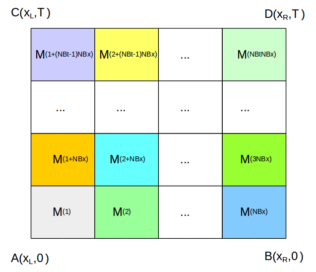 Figure 1
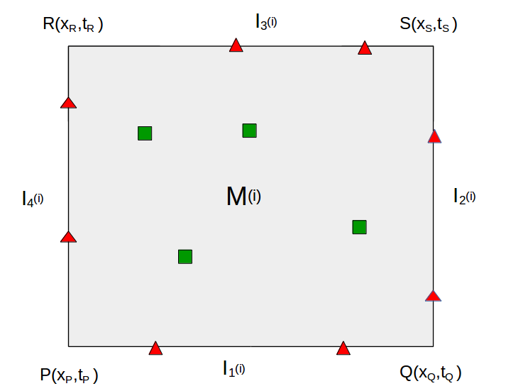 Figure 2
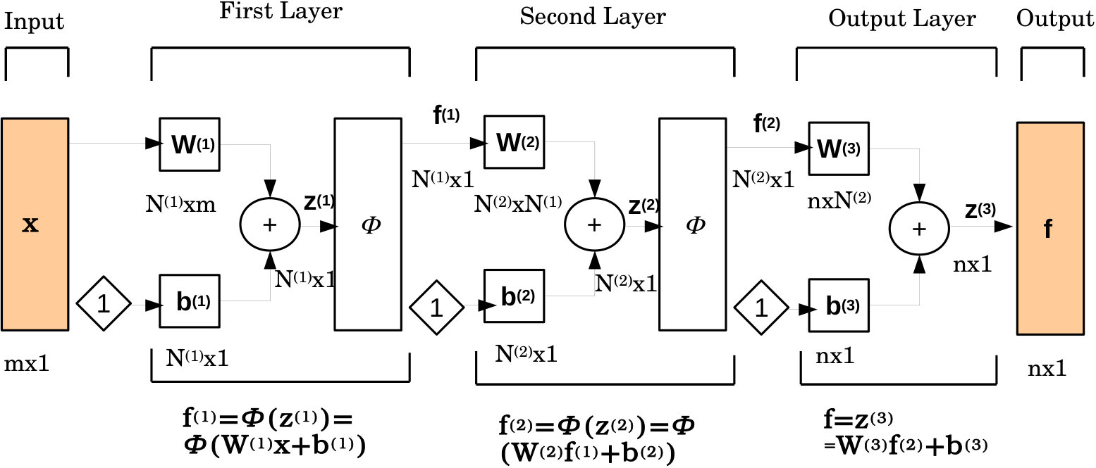 Figure 3
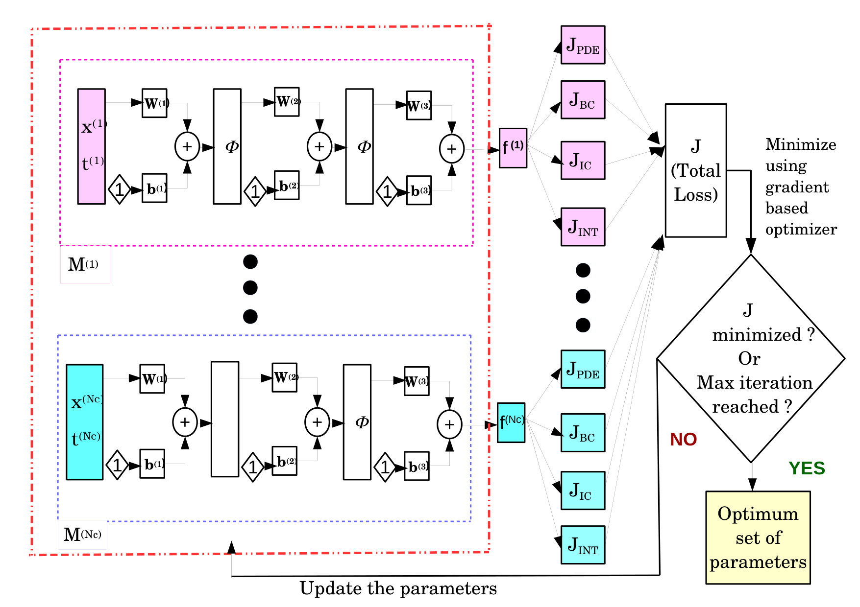 Figure 4
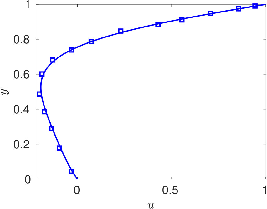 Figure 5
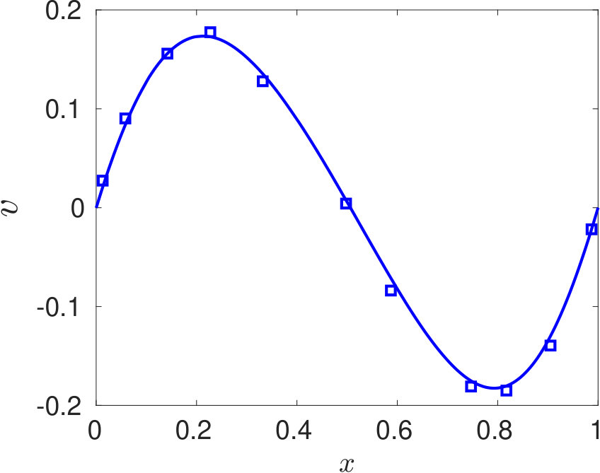 Figure 6
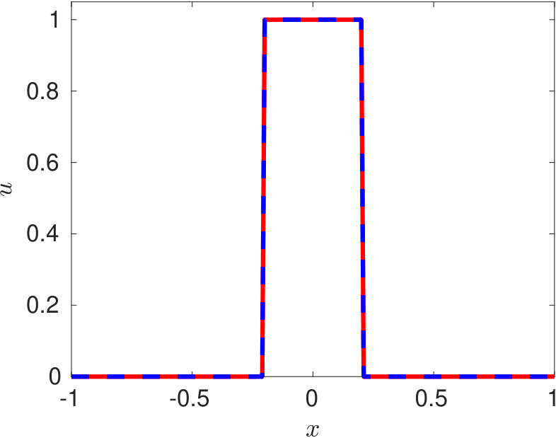 Figure 7
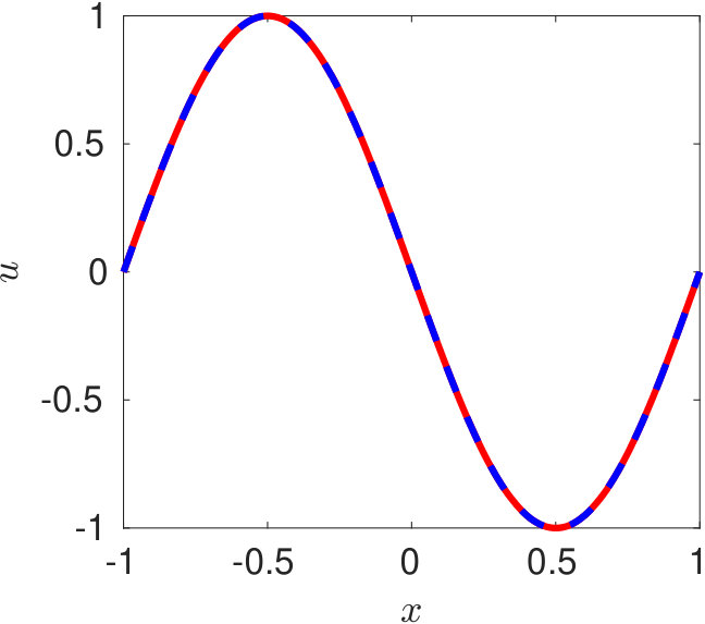 Figure 8
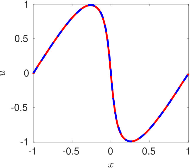 Figure 9
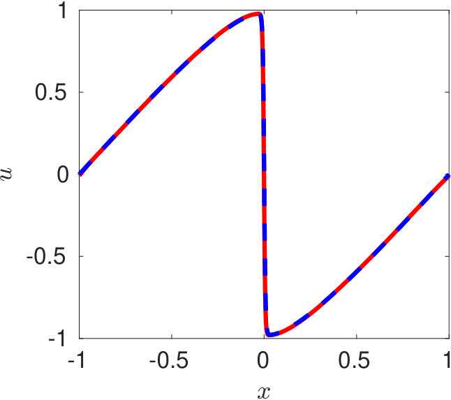 Figure 10
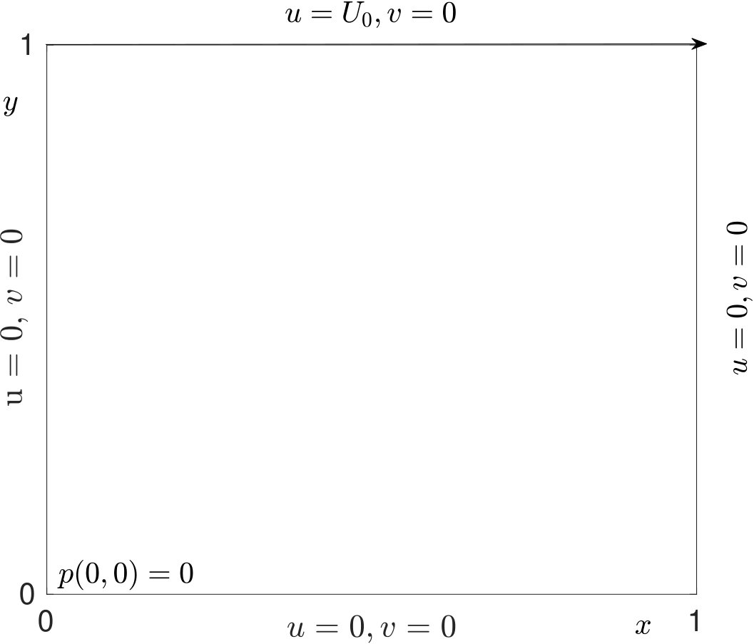 Figure 11
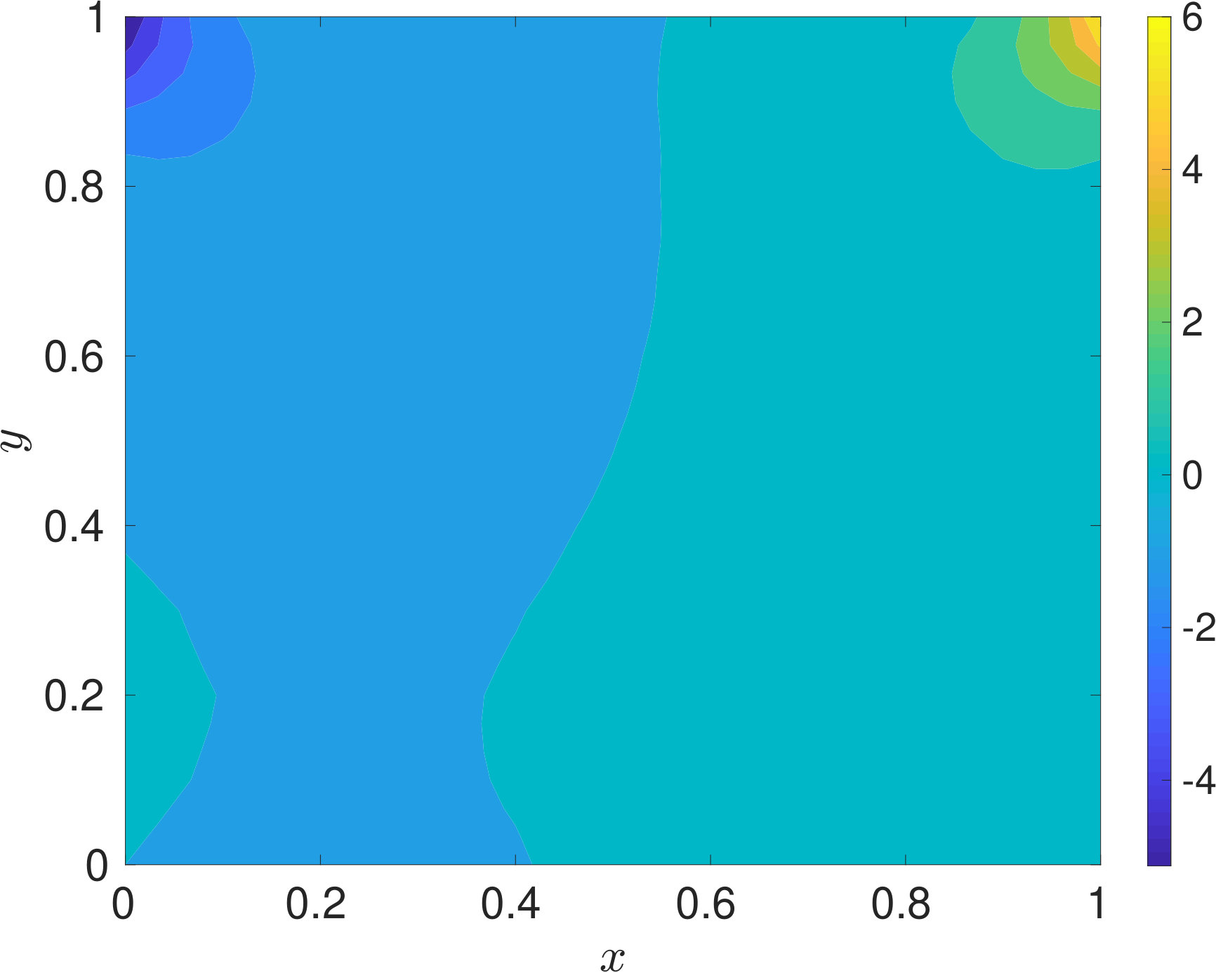 Figure 12
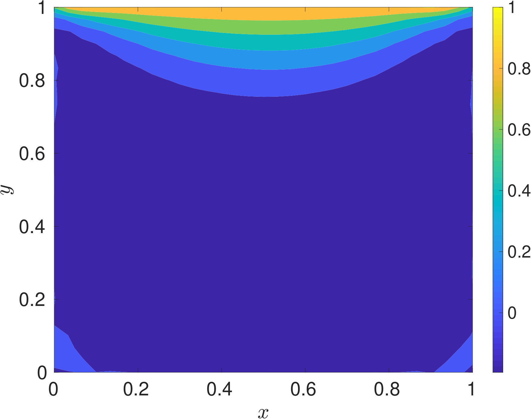 Figure 13
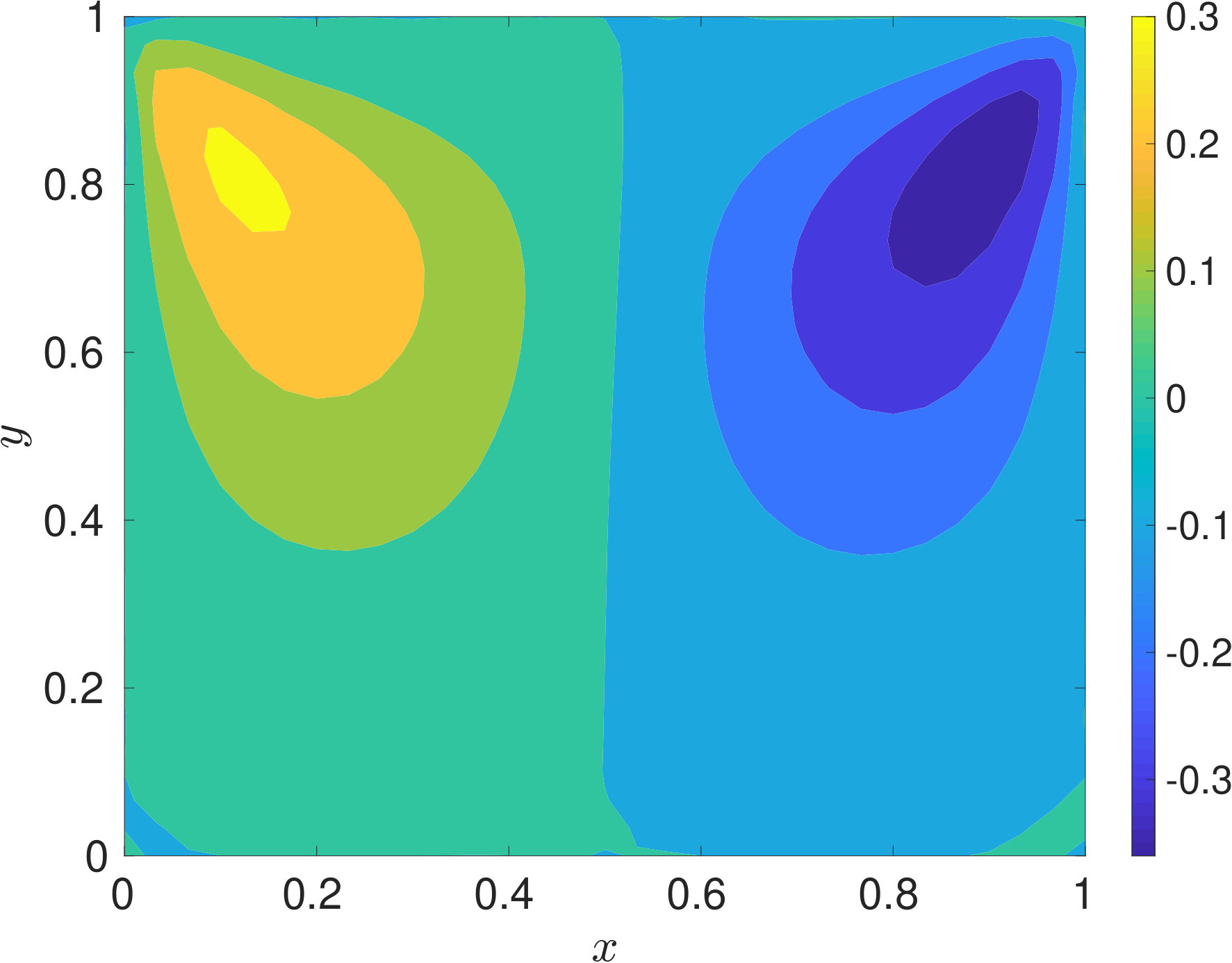 Figure 14
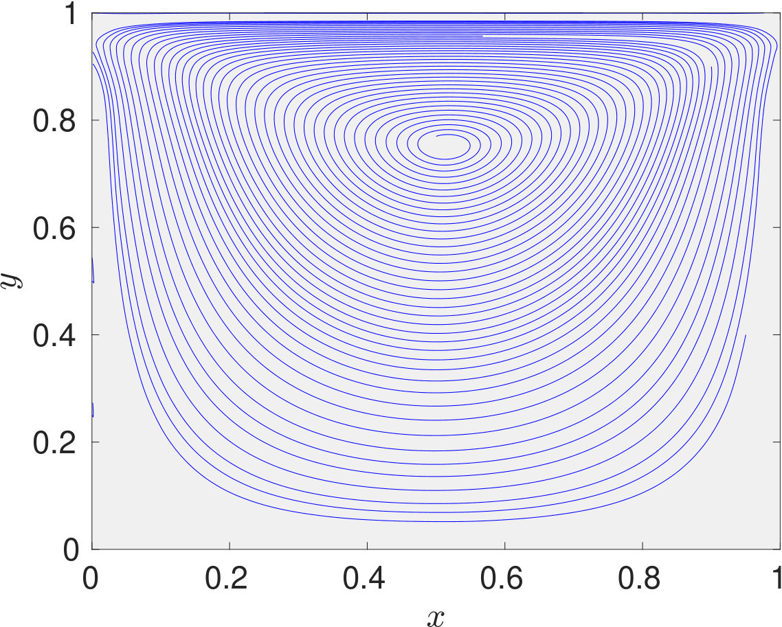 Figure 15
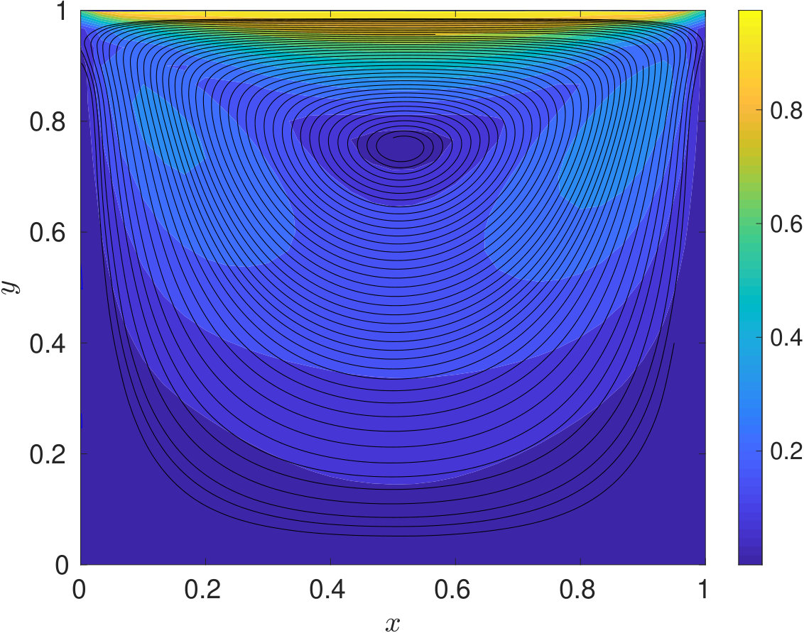 Figure 16
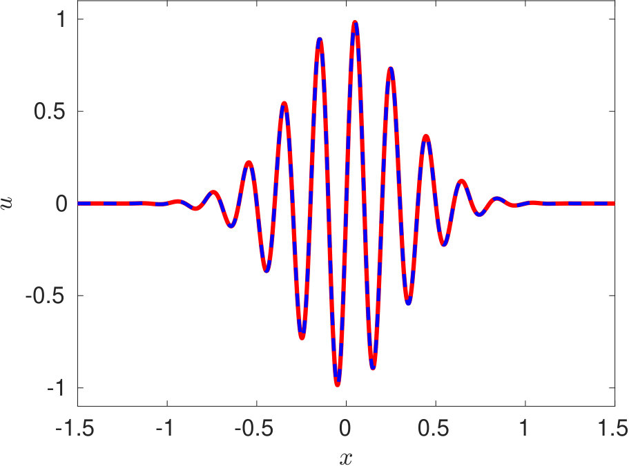 Figure 17
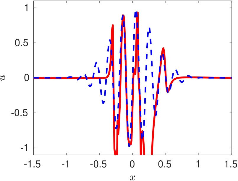 Figure 18
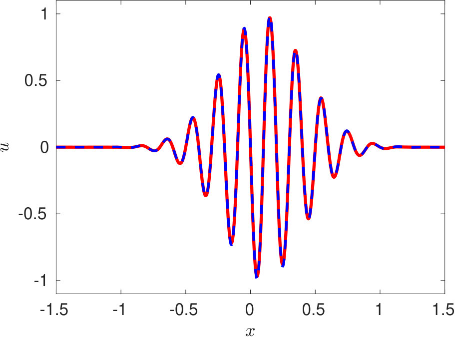 Figure 19
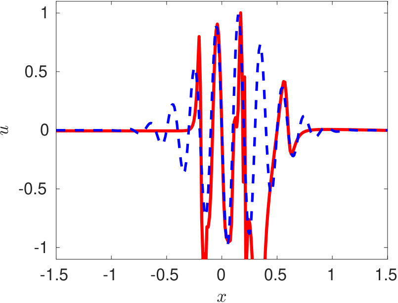 Figure 20
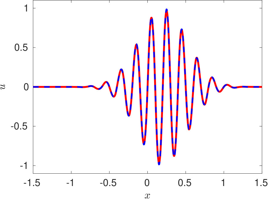 Figure 21
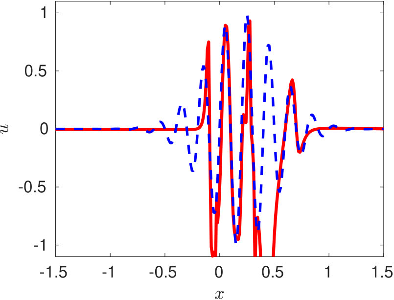 Figure 22
Peer Reviews
No public reviews on file for this paper yet. If you reviewed it on a platform where reviews are public (OpenReview, ICLR, NeurIPS, ICML), you can paste yours below so the community can read it here.
Videos
No videos yet. Explain this paper in a talk, walkthrough, or lecture? Add one.
Distributed physics informed neural network for data-efficient solution to partial differential equations
Vikas Dwivedi
Nishant Parashar
Balaji Srinivasan
Department of Mechanical Engineering, Indian Institute of Technology Madras, Chennai 600036, India
Department of Applied Mechanics, Indian Institute of Technology Delhi, New Delhi 110016, India
Abstract
The physics informed neural network (PINN) is evolving as a viable method to solve partial differential equations. In the recent past PINNs have been successfully tested and validated to find solutions to both linear and non-linear partial differential equations (PDEs). However, the literature lacks detailed investigation of PINNs in terms of their representation capability. In this work, we first test the original PINN method in terms of its capability to represent a complicated function. Further, to address the shortcomings of the PINN architecture, we propose a novel distributed PINN, named DPINN. We first perform a direct comparison of the proposed DPINN approach against PINN to solve a non-linear PDE (Burgers’ equation). We show that DPINN not only yields a more accurate solution to the Burgers’ equation, but it is found to be more data-efficient as well. At last, we employ our novel DPINN to two-dimensional steady-state Navier-Stokes equation, which is a system of non-linear PDEs. To the best of the authors’ knowledge, this is the first such attempt to directly solve the Navier-Stokes equation using a physics informed neural network.
keywords:
Machine learning, Deep neural networks, Physics informed neural networks, Burgers’ equation, Navier Stokes equation,
1 Introduction
Partial differential equations (PDEs) are extensively used in the mathematical modelling of a variety of problems in physics, engineering and finance. For a variety of practical problems of interest, the analytical solution of these PDEs is generally unknown. Over the years, various numerical methods have been developed to solve these PDEs. Most of the popular numerical methods viz. finite element method Rao [2017], finite difference method LeVeque [2007] and finite volume method Versteeg & Malalasekera [2007] are mesh-based methods. Although these numerical methods are very successful and are widely used, there are various problems associated with these methods. For example, it is a well-known fact that mesh generation is a very difficult task with complex geometries. Furthermore, the discretisation of the PDE itself introduces truncation errors, which can be a quite serious problem Quirk [1997].
With the recent advances in the computational resources and availability of data, the deep neural networks have evolved as a viable method to solve PDEs. The performance of a neural network in solving PDEs depends on two main factors: (1) neural network architecture and (2) learning algorithms. As a result, the design of new neural network architectures and learning algorithms has become an active area of research for the past decade. Recently, Berg & Nyström [2018] have produced good results in solving stationary PDEs with complex geometries and Sirignano & Spiliopoulos [2018] have introduced a deep Galerkin method to solve high dimensional PDEs. We also refer to the earlier works of Lagaris et al. [1998, 2000] in which they solved the initial boundary value problem using neural networks and later extended their work to handle irregular boundaries. Since then, a lot of researchers have made their contributions in solving initial and boundary value problems in arbitrary boundaries McFall & Mahan [2009], Kumar & Yadav [2011], Mall & Chakraverty [2016].
Among all the deep neural network-based approaches to solve PDEs, we particularly refer to the physics-informed learning machines which have shown promising results for a series of nonlinear benchmark problems. The peculiar property of this approach is the inclusion of the prior-structured information about the solution in the learning algorithm. The initial promising results using this method were reported by Owhadi [2015], Raissi et al. [2017a, b]. The authors employed the Gaussian process regression to accurately infer the solutions to linear problems along with the associated uncertainty estimates. Further, their method was extended to nonlinear problems by Raissi & Karniadakis [2018] and Raissi et al. [2018] in the context of both inference and system identification. Finally, the physics informed neural networks (PINN) are introduced by Raissi et al. [2019] for both data-driven solution of PDEs as well as the data-driven discovery of parameters in a PDE.
Although PINNs have been successfully tested to retrieve accurate solutions for a wide variety of PDEs, they suffer from several drawbacks Raissi et al. [2019]. For example (i) the required depth of the PINN increases with increasing order of PDE leading to slow learning-rate due to the well-known issue of vanishing gradients, (ii) PINNs are not robust in representing sharp local gradients in a broad computational domain Dwivedi & Srinivasan [2019]. In addition to this, there is a lot of uncertainty in terms of requirement of the amount of training data and the number of hidden layers for efficient implementation of the PINN.
In this paper, we propose a distributed version of the original PINN called distributed PINN (or DPINN). The DPINN handles several issues encountered by the original PINN Raissi et al. [2019] by efficiently designing the network architecture and modifying the associated cost function. In the DPINN approach, the computational domain is distributed into smaller sub-domains (called cells), and simpler PINNs are employed in each of these individual cells. These individual PINNs (in the comprehensive DPINN) are just two layers deep. Hence, solving the potential vanishing gradients issue of using deeper PINNs. Although this partitioning complicates the cost function as we have to penalise for the interfacial flux mismatch across the neighbouring cells, still it simplifies the function or PDE to be represented by the local PINN. This makes DPINN more data-efficient in comparison to the original PINN.
This paper is organised into five sections. In Section 2 we, present a brief overview of the physics informed neural network (PINN) of Raissi et al. [2019]. The proposed novel DPINN architecture, along with the mathematical formulation, is described in Section 3. The detailed evaluation of DPINN, in terms of its representation capability and the ability to solve non-linear PDEs in performed in Section 4. Section 5 concludes the work with a summary.
2 Review of physics informed neural network
Raissi et al. [2019] proposed a data-efficient PINN network for approximating solutions to general non-linear PDEs and validated it with a series of benchmark test cases. The main feature of the PINN is the inclusion of the prior knowledge of physics in the learning algorithm as cost function. As a result, the algorithm imposes a penalty for any non-physical solution and quickly directs it towards the correct solution. This physics informed approach enhances the information content of the data. As a result, the algorithm has good generalization property even in the small data set regime.
2.0.1 Mathematical formulation
Consider a PDE of the following form:
[TABLE]
[TABLE]
[TABLE]
where may be a linear or nonlinear differential operator and is the boundary of computational domain . We approximate with the output of the neural network.
For simplicity, a schematic diagram of a simple two layer deep neural network with an input and an output is shown in Fig 1. In this case, assuming , the neural network output is given by:
[TABLE]
where is the activation function and and represent the weight matrix and bias vector of layer. The expression for deeper networks can also be written in a similar fashion. The essence of PINN lies in the definition of its loss function. In order to make the neural network “physics informed”, the loss function is defined such that a penalty is imposed whenever the network output doesn’t respect the physics of the problem. If we denote the training errors in approximating the PDE, BCs and IC by , and respectively. Then, the expressions for these errors are as follows:
[TABLE]
[TABLE]
[TABLE]
The expressions for and used in the equation (5) can be computed using automatic differentiation Baydin et al. [2017]. The loss function to be minimized for a PINN is given by
[TABLE]
where , and correspond to losses at collocation, boundary condition and initial condition data respectively. The expressions for these losses are given below:
[TABLE]
[TABLE]
[TABLE]
where , and refer to number of collocation points, boundary condition points and initial condition points respectively. Finally, any gradient-based optimization routine may be used to minimize . This completes the mathematical formulation of PINN. The key steps in its implementation are as follows:
Identify the PDE to be solved along with the initial and boundary conditions. 2. 2.
Decide the architecture of PINN. 3. 3.
Approximate the correct solution with PINN. 4. 4.
Find expressions for the PDE, BCs and IC in terms of PINN and its derivatives. 5. 5.
Define a loss function which penalizes for error in PDE, BCs and IC. 6. 6.
Minimize the loss with gradient-based algorithms.
3 Distributed PINN
In this section, we propose a distributed version of PINN called DPINN. This algorithm takes motivation from finite volume methods in which the whole computational domain is partitioned into multiple cells, and the governing equations are solved for each cell. The solutions of these individual cells are stitched together with additional convective and diffusive fluxes conditions at the cell interfaces. We adopt a similar strategy in DPINN. As the representation of a complex function is very hard for a single PINN in the whole domain, we divide the domain into multiple cells and install a PINN in each cell. Therefore, each PINN uses different representations in different portions of the domain while satisfying some additional constraints of continuity and differentiability. In the conventional PINNs, the prior information of the physics of the problem acts as a regularizer in a global sense. However in the DPINN approach, the additional interface conditions act as local regularization agents that further constrain the space of admissible solution.
3.1 Mathematical formulation
Consider the following 1D unsteady problem
[TABLE]
[TABLE]
[TABLE]
where is a potentially nonlinear differential operator and is the boundary of computational domain . In this problem, the rectangular domain is given by . On uniformly dividing into non-overlapping rectangular cells, may be written as
[TABLE]
The boundary of the cell is denoted by . For rectangular cells,
[TABLE]
where represents the interface of .
Fig (2a) shows the distribution of PINNs in a rectangular computational domain with cells (i.e. ). We denote the PINN on the cell by . Fig (2b) shows a PINN with collocation points at the interior and the boundary points at the four interfaces. Each individual PINN has its own set of weights and biases. The output corresponding to a given is denoted by .
At each , we enforce additional constraints of continuity (or smoothness) of solution at the cell interfaces depending on the differential operator . For example, continuity of solution is sufficient for advection problems. For the diffusion problem, the solution should be continuously differentiable. For the computational domain shown in figure (2), the loss function to be minimized is a combination of conventional PINN losses and additional interface losses and is given by:
[TABLE]
Figure 3 presents a detailed schematic of the DPINN architecture.
3.1.1 Expressions for the conventional PINN losses
[TABLE]
[TABLE]
[TABLE]
where , , , , , , and .
3.1.2 Expressions for the additional interface losses
In general, we consider total interface loss as sum of continuity and differentiability losses i.e.
[TABLE]
where , refer to continuity losses along and interfaces and refers to differentiability loss along interfaces. The expressions for these losses are as follows:
[TABLE]
[TABLE]
[TABLE]
where
[TABLE]
[TABLE]
[TABLE]
, and
It is to be noted that although we have shown the formulation for 1D unsteady problems, no special adjustment is needed to extend the formulation to higher dimensional problems. This completes the mathematical formulation of DPINN. The main steps in its implementation are as follows:
Divide the computational domain into uniformly distributed non-overlapping cells and install a PINN in each cell. 2. 2.
Depending on the cell location, PDE and the initial and boundary conditions, find the conventional PINN losses at each cell. 3. 3.
Depending on the PDE, calculate interface losses at each cell interface. 4. 4.
Calculate the total loss by taking the summation of all the losses. 5. 5.
Minimize the total loss using a gradient descent algorithm.
4 Results and Discussions
In this section, we first test the original PINN developed by Raissi et al. [2019] in terms of its ability to represent complicated functions. In this regard, we employ the PINN to solve the advection equation with complex initial conditions. After that, we discuss the bottlenecks of the PINN and explain how the proposed DPINN is an improvement over the PINN. Further, we evaluate the performance of DPINNs in solving non-linear PDEs as well. We first test our network for predicting the solution to the Burgers’ equation. The performance is evaluated in terms of accuracy as compared to numerically accurate solutions and the PINN of Raissi et al. [2019]. After that, we evaluate our model on a system of non-linear PDEs, namely, the Navier Stokes equations and validate the results against well-established results of Ghia et al. [1982].
For all the problems presented in this work, we have used the non-linear activation function. The Adam optimizer Kingma & Welling [2014], is kept as the default optimizer throughout this work. The learning rate is 0.001 for advection and Burgers’ equation and 0.0001 for the Navier Stokes equation. The input data in all of the individual cells of the DPINN is normalised in the range .
4.1 Advection equation
In this section, we first present the solution of the advection equation obtained using the PINN. In one-dimension, the advection equation has the following mathematical form:
[TABLE]
where is the velocity field at time , along the -direction. There are two basic motivations for choosing advection equation as a primary testbed for evaluating the PINN (i) to test the ability of PINN to accurately represent complicated initial conditions and (ii) to test its ability to robustly translate a complex initial profile. Both of these characteristics are essential to retrieve a space and time continuous solution to an unsteady partial differential equation. We choose a complex initial velocity profile :
[TABLE]
We use the open-source PINN solver available on https://github.com/maziarraissi/PINNs. Training of the PINN is performed on 25,600 collocation points. In figure 4, we show the solution obtained using PINN at three time-instants. It can be observed that the conventional PINN approach fail to even represent the initial profile at (equation 26).
In the conventional PINN, the position of the collocation points is random in the absence of any residual adaptive refinement. For the complicated representation of this type, we need a larger amount of training data in the regions of sharp gradients. However, this information is not known to us apriori. The cost function of the conventional PINN acts as a regularizer but only in a global sense. Therefore it is very hard for the algorithm to capture these sharp local variations in a wide computational domain. The use of an even deeper network and a larger number of collocation points would be required to train for such complicated profiles. However, using a deeper network might restrain the training speed due to a well-known issue of vanishing gradients.
To overcome these bottlenecks of PINN, we propose a new DPINN architecture as discussed in section 3. The DPINN approach mitigates the above-mentioned limitations of PINN by introducing additional interface conditions, which act as a local regularization agent. This interface loss compensates for the shortage of training data in each cell. Further, the sampling of collocation points is more efficient in the DPINN architecture as compared to the original PINN as each cell now contains the same number of data points. With these motivations, we train the DPNN to solve the advection equation. The computational domain is distributed into 25 equally spaced cells along -direction and five cells along -axis. A neural network is employed on each of these cells. Each of these distributed neural networks is trained on 45 equally spaced collocation points using a two-layer network with five neurons in each layer. In figure 5 we present the solution of the advection equation 25 obtained using DPINN. These plots (figure 5) are obtained at three different time instants using a separate testing data-set of 4,221 unique collocation points. The mean-squared errors for the solutions presented in figure 5 is .
In summary, the observed robustness of the proposed DPINN architecture can be attributed to the use of simpler neural networks over various segments of the computational domain. The DPINN basically tries to approximate a complicated spatio-temporal profile, by using piece-wise simpler neural networks. Such simpler neural networks are easier to train as compared to the original PINN architecture proposed by Raissi et al. [2019].
4.2 Burgers’ equation
In this section, we demonstrate a direct comparison of the proposed DPINN against the original PINN in terms of the accuracy of the predicted solution. For this, we compare the solution to the Burgers’ equation obtained using DPINN against that of Raissi et al. [2019]. Burgers’ equation is a non-linear partial differential equation. It is considered to be a canonical test case to demonstrate the ability of any numerical scheme to capture shocks/discontinuities in the flow field. The Burgers’ equation in one-dimension can be expressed as:
[TABLE]
Raissi et al. [2019] employed the PINN network to find solution to the Burgers’ equation corresponding to a sinusodial initial condition:
[TABLE]
In figure 6, we present the solution obtained at three different time instants using DPINN. The training of DPINN is performed using 4,141 collocation points. These points were distributed in 25 equally spaced cells along -direction and ten equally spaced cells along -axis. We use a two-layer neural network for each distributed domain with five neurons in each layer. The predicted solution (figure 6) is obtained on 1,001 collocation points with a relative L2-norm error of -.
Raissi et al. [2019] trained their PINN on various configurations and reported a maximum accuracy while training on collocation points using an eight-layer deep network with 40 neurons per layer. They reported a minimum relative L2-norm error of -. On the other hand, by using distributed simpler neural networks DPINN achieves a smaller prediction error while training on a smaller dataset ( the data required for PINN). Hence besides being computationally more accurate, the DPINN architecture has been found to be more data-efficient as compared to the PINN architecture.
4.3 Navier-Stokes equation
In this section we go a step ahead in testing the DPINN to find solution to a system of non-linear partial differential equations. The Navier Stokes equation is a system of partial differential equations and is considered to be one of the most challenging equation to solve. We choose to solve the equations to find the velocity and pressure field inside a two-dimensional square cavity with a moving top plate (lid driven cavity problem), as shown in figure 7. At a smaller Reynolds number, this flow is known to possess a incompressible steady state solution. Hence, we can directly simplify the Navier stokes equation, to yield the steady state solution by removing the temporal term. Further, we impose the divergence-free incompressibility condition to arrive at the following form:
[TABLE]
where, u and v are the velocity component along the x and y direction, is the pressure, represents the kinematic viscosity and is the fluid density. Equation (29) is the continuity equation, while equations (30) and (31) represents the momentum equations.
Although these equations have been simplified, they still are, in their presented form, a highly non-linear system of parital differential equations. To the best of our knowledge, this is the first such attempt to directly solve the Navier-Stokes equation directly using a PINN based approach.
Since, for the problem of interest, the flow is incompressible, density can be assumed to be constant. Hence, we would train our proposed DPINN to retrieve the pressure and velocity field only. The problem domain and the boundary conditions are specified in figure 7. The Reynolds number of the flow is 10 (, where L is length of the plate). The training of the DPINN is performed using 961 collocation points. These points are distributed in ten equally spaced cells along -direction and -direction. We use a two-layer neural network for each distributed domain with five neurons in each layer. In figure 8, we show the predictions obtained using DPINN. The -velocity obtained at the centerline is presented in 6(a) and -velocity obtained at the centerline is presented in 6(b). Both of these results are compared against well-established results of Ghia et al. [1982]. It can be observed that both the centerline velocities obtained using DPINN are in good agreement with the results of Ghia et al. [1982]. Further, in figure 8(c) we show the streamlines and in figures 8(d), 8(e) and 8(f) we show velocity and pressure contours obtained using DPINN. These contours and streamlines depict the physical flow pattern that is expected to form for this flow problem.
Although, for the presented problem, DPINNs have been able to find the solution to the Navier-Stokes equation. We want to clarify that, the flow problem simulated in this work (lid-driven cavity) has a low Reynolds number. With increasing Reynolds number, the complexity of the solution increases since the flow becomes unsteady, turbulent and three-dimensional. The current work sets the foundation for the use of DPINNs to directly solve the Navier-Stokes equations and is, in fact, the first such attempt in this direction.
5 Conclusions
In this paper, we present DPINNa data-efficient distributed version of PINN to solve linear as well as nonlinear PDEs. The proposed DPINN enhances the capability of PINN by improving both its network architecture and the employed learning algorithm. DPINN incorporates a divide-and-conquer type strategy analogous to finite volume methods by partitioning the computational domain into smaller sub-domains (called cells) and installing a local PINN in each of these cells. This partitioning breaks the hard problem which potentially requires a very deep PINN, into smaller sub-problems which can be solved by various minimal sized local PINNs. The additional physical constraints at the interfaces act as natural network regularizers, which boosts the representation capability of the network. The cost function of DPINN itself stitches the individual local PINN solutions, which makes DPINN even more data-efficient than the original PINN.
The major highlights of this study are as follows:
We have proposed a novel improved PINN algorithm (called DPINN) which is more data-efficient and addresses the vanishing gradient issue encountered by deep PINNs. 2. 2.
We provide a glimpse of the improved representation power of DPINN by employing it to solve the advection equation. We find that while PINN fails even to represent a high-frequency wave packet, DPINNs not just accurately represents the wave packet, but robustly advects it as well. 3. 3.
We show that DPINN yields a more accurate solution to the Burgers’ equation with a smaller amount of training data as compared to the PINN solution. 4. 4.
We show that DPINNs can be used to solve steady-state Navier-Stokes equations at low Reynolds number. However, to solve unsteady full three-dimensional Navier-Stokes equations, a more detailed analysis needs to be performed. However, such a study will require more advancements in the algorithm and larger computational resources, which is beyond the scope of the present work.
This paper has demonstrated that DPINNs can be efficiently used to find data-driven solution to PDEs. The next obvious task in this direction is to extend the DPINN approach for the inverse problem, ie. data-driven discovery of PDEs. We are currently working in this direction and will report consequent progress in our future work.
References
- Baydin et al. [2017]
Baydin, A. G., Pearlmutter, B. A., Radul, A. A., & Siskind, J. M. (2017).
Automatic differentiation in machine learning: A survey.
J. Mach. Learn. Res., 18, 5595–5637. URL: http://dl.acm.org/citation.cfm?id=3122009.3242010.
- Berg & Nyström [2018]
Berg, J., & Nyström, K. (2018).
A unified deep artificial neural network approach to partial differential equations in complex geometries.
Neurocomputing, 317, 28–41. doi:10.1016/j.neucom.2018.06.056.
- Dwivedi & Srinivasan [2019]
Dwivedi, V., & Srinivasan, B. (2019).
Physics Informed Extreme Learning Machine (PIELM) – A rapid method for the numerical solution of partial differential equations.
arXiv e-prints, (p. arXiv:1907.03507). arXiv:1907.03507.
- Ghia et al. [1982]
Ghia, U., Ghia, K. N., & Shin, C. (1982).
High-re solutions for incompressible flow using the navier-stokes equations and a multigrid method.
J. Comput. Phys., 48, 387--411. doi:10.1016/0021-9991(82)90058-4.
- Kingma & Welling [2014]
Kingma, D. P., & Welling, M. (2014).
An introduction to variational autoencoders.
arXiv e-prints, .
- Kumar & Yadav [2011]
Kumar, M., & Yadav, N. (2011).
Multilayer perceptrons and radial basis function neural network methods for the solution of differential equations: a survey.
Comput Math Appl, 62, 3796--3811. doi:10.1016/j.camwa.2011.09.028.
- Lagaris et al. [1998]
Lagaris, I. E., Likas, A., & Fotiadis, D. I. (1998).
Artificial neural networks for solving ordinary and partial differential equations.
IEEE Trans. Neural Netw., 9, 987--1000. doi:10.1109/72.712178.
- Lagaris et al. [2000]
Lagaris, I. E., Likas, A. C., & Papageorgiou, D. G. (2000).
Neural-network methods for boundary value problems with irregular boundaries.
IEEE Trans. Neural Netw., 11, 1041--1049. doi:10.1109/72.870037.
- LeVeque [2007]
LeVeque, R. J. (2007).
Finite difference methods for ordinary and partial differential equations: steady-state and time-dependent problems volume 98.
Siam.
- Mall & Chakraverty [2016]
Mall, S., & Chakraverty, S. (2016).
Application of legendre neural network for solving ordinary differential equations.
Appl. Soft Comput., 43, 347--356. doi:10.1016/j.asoc.2015.10.069.
- McFall & Mahan [2009]
McFall, K. S., & Mahan, J. R. (2009).
Artificial neural network method for solution of boundary value problems with exact satisfaction of arbitrary boundary conditions.
IEEE Trans. Neural Netw., 20, 1221--1233. doi:10.1109/TNN.2009.2020735.
- Owhadi [2015]
Owhadi, H. (2015).
Bayesian numerical homogenization.
Multiscale Model Simul, 13, 812--828. doi:10.1137/140974596.
- Quirk [1997]
Quirk, J. J. (1997).
A contribution to the great riemann solver debate.
In Upwind and High-Resolution Schemes (pp. 550--569).
Springer.
- Raissi & Karniadakis [2018]
Raissi, M., & Karniadakis, G. E. (2018).
Hidden physics models: Machine learning of nonlinear partial differential equations.
J. Comput. Phys., 357, 125--141. doi:10.1016/j.jcp.2017.11.039.
- Raissi et al. [2017a]
Raissi, M., Perdikaris, P., & Karniadakis, G. E. (2017a).
Inferring solutions of differential equations using noisy multi-fidelity data.
J. Comput. Phys., 335, 736--746. doi:10.1016/j.jcp.2017.01.060.
- Raissi et al. [2017b]
Raissi, M., Perdikaris, P., & Karniadakis, G. E. (2017b).
Machine learning of linear differential equations using gaussian processes.
J. Comput. Phys., 348, 683--693. doi:10.1016/j.jcp.2017.07.050.
- Raissi et al. [2018]
Raissi, M., Perdikaris, P., & Karniadakis, G. E. (2018).
Numerical gaussian processes for time-dependent and nonlinear partial differential equations.
SIAM J SCI COMPUT, 40, A172--A198. doi:10.1137/17M1120762.
- Raissi et al. [2019]
Raissi, M., Perdikaris, P., & Karniadakis, G. E. (2019).
Physics-informed neural networks: A deep learning framework for solving forward and inverse problems involving nonlinear partial differential equations.
J. Comput. Phys., 378, 686--707. doi:10.1016/j.jcp.2018.10.045.
- Rao [2017]
Rao, S. S. (2017).
The finite element method in engineering.
Butterworth-heinemann.
- Sirignano & Spiliopoulos [2018]
Sirignano, J., & Spiliopoulos, K. (2018).
Dgm: A deep learning algorithm for solving partial differential equations.
J. Comput. Phys., 375, 1339--1364. doi:10.1016/j.jcp.2018.08.029.
- Versteeg & Malalasekera [2007]
Versteeg, H. K., & Malalasekera, W. (2007).
An introduction to computational fluid dynamics: the finite volume method.
Pearson education.
The reference list from the paper itself. Each links out to its DOI / PubMed record.
- 1Baydin et al. [2017] Baydin, A. G., Pearlmutter, B. A., Radul, A. A., & Siskind, J. M. (2017). Automatic differentiation in machine learning: A survey. J. Mach. Learn. Res. , 18 , 5595–5637. URL: http://dl.acm.org/citation.cfm?id=3122009.3242010 .
- 2Berg & Nyström [2018] Berg, J., & Nyström, K. (2018). A unified deep artificial neural network approach to partial differential equations in complex geometries. Neurocomputing , 317 , 28–41. doi: 10.1016/j.neucom.2018.06.056 . · doi ↗
- 3Dwivedi & Srinivasan [2019] Dwivedi, V., & Srinivasan, B. (2019). Physics Informed Extreme Learning Machine (PIELM) – A rapid method for the numerical solution of partial differential equations. ar Xiv e-prints , (p. ar Xiv:1907.03507). ar Xiv:1907.03507 .
- 4Ghia et al. [1982] Ghia, U., Ghia, K. N., & Shin, C. (1982). High-re solutions for incompressible flow using the navier-stokes equations and a multigrid method. J. Comput. Phys. , 48 , 387--411. doi: 10.1016/0021-9991(82)90058-4 . · doi ↗
- 5Kingma & Welling [2014] Kingma, D. P., & Welling, M. (2014). An introduction to variational autoencoders. ar Xiv e-prints , .
- 6Kumar & Yadav [2011] Kumar, M., & Yadav, N. (2011). Multilayer perceptrons and radial basis function neural network methods for the solution of differential equations: a survey. Comput Math Appl , 62 , 3796--3811. doi: 10.1016/j.camwa.2011.09.028 . · doi ↗
- 7Lagaris et al. [1998] Lagaris, I. E., Likas, A., & Fotiadis, D. I. (1998). Artificial neural networks for solving ordinary and partial differential equations. IEEE Trans. Neural Netw. , 9 , 987--1000. doi: 10.1109/72.712178 . · doi ↗
- 8Lagaris et al. [2000] Lagaris, I. E., Likas, A. C., & Papageorgiou, D. G. (2000). Neural-network methods for boundary value problems with irregular boundaries. IEEE Trans. Neural Netw. , 11 , 1041--1049. doi: 10.1109/72.870037 . · doi ↗