A two-patch epidemic model with nonlinear reinfection
Juan G. Calvo, Alberto Hern\'andez, Mason A. Porter, and Fabio Sanchez

TL;DR
This paper develops a two-patch epidemic model with nonlinear reinfection to analyze how movement between urban and rural populations influences disease spread and stability, highlighting potential benefits of population movement in controlling outbreaks.
Contribution
It introduces a novel two-patch SI extasciitilde S model with nonlinear reinfection and analyzes the effects of population movement on disease dynamics and stability.
Findings
Population movement can expand the stability region of disease-free states.
Nonlinear reinfection significantly affects disease persistence.
Movement between patches can be beneficial for disease control.
Abstract
The propagation of infectious diseases and its impact on individuals play a major role in disease dynamics, and it is important to incorporate population heterogeneity into efforts to study diseases. As a simplistic but illustrative example, we examine interactions between urban and rural populations in the dynamics of disease spreading. Using a compartmental framework of susceptible--infected--susceptible () dynamics with some level of immunity, we formulate a model that allows nonlinear reinfection. We investigate the effects of population movement in the simplest scenario: a case with two patches, which allows us to model movement between urban and rural areas. To study the dynamics of the system, we compute a basic reproduction number for each population (urban and rural). We also compute steady states, determine the local stability of the disease-free…
Click any figure to enlarge with its caption.
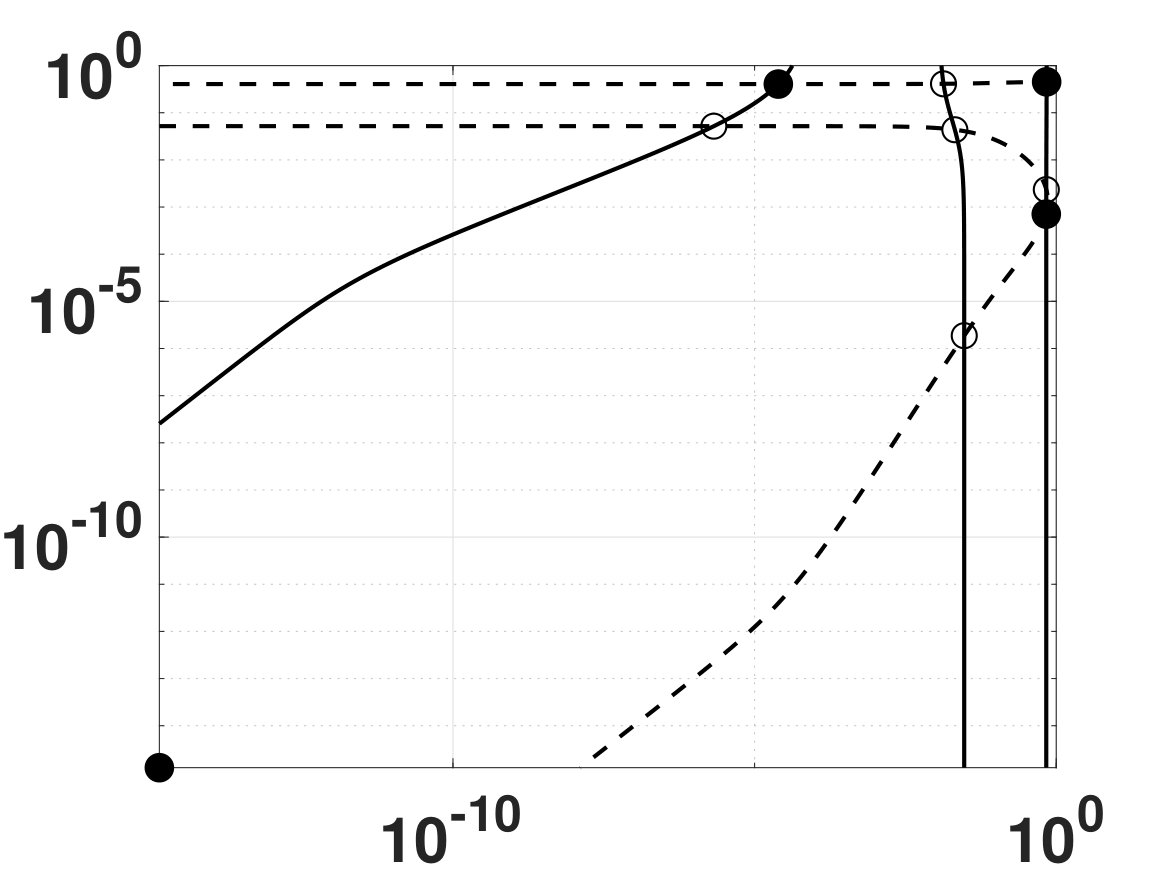 Figure 1
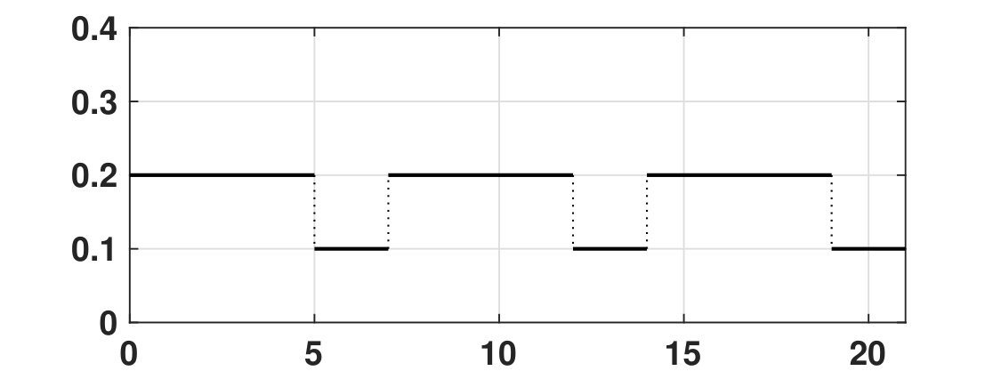 Figure 2
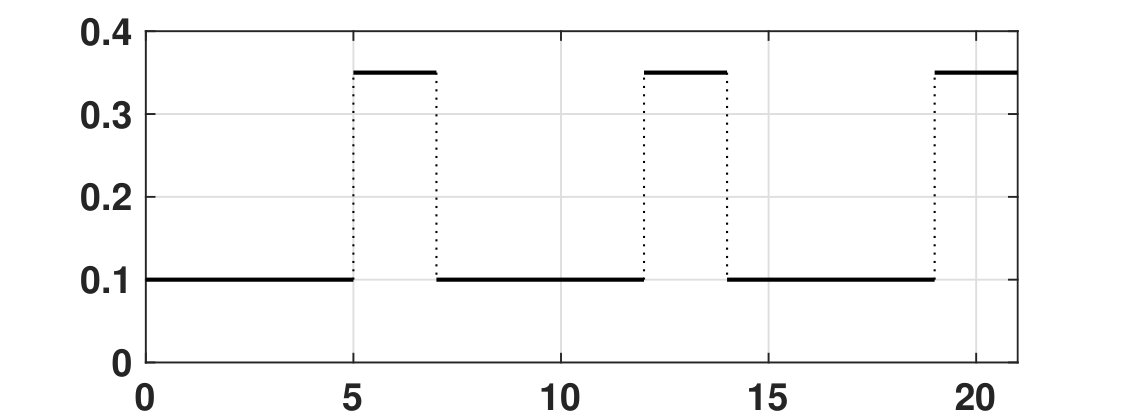 Figure 3
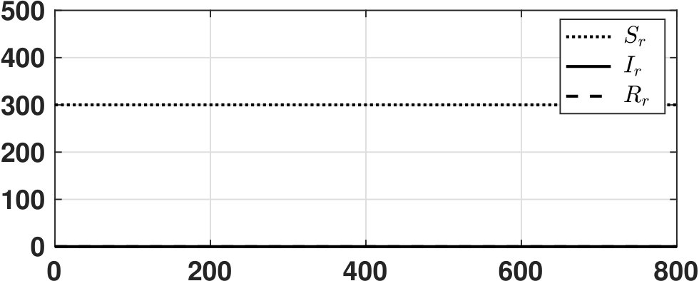 Figure 4
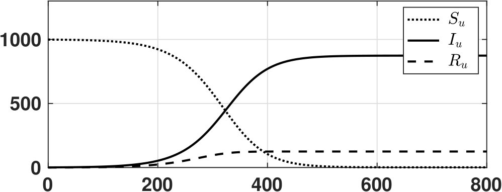 Figure 5
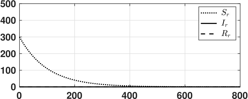 Figure 6
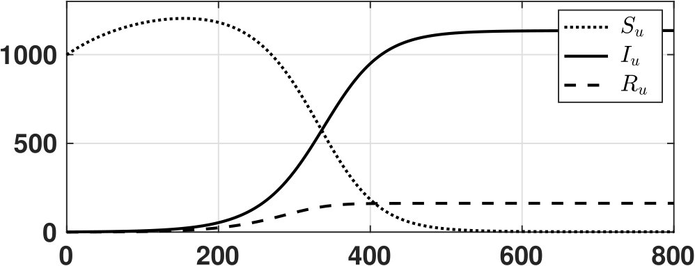 Figure 7
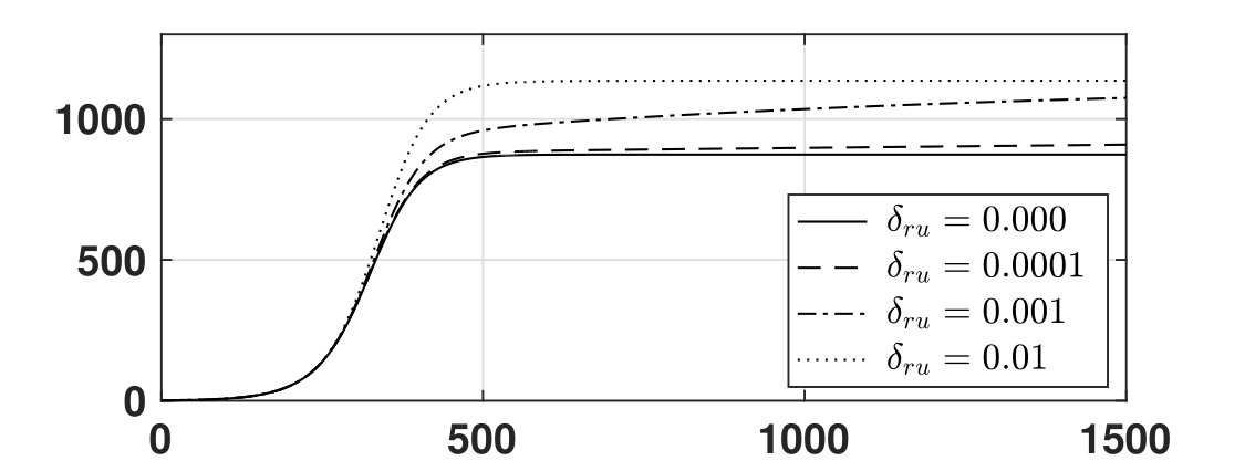 Figure 8
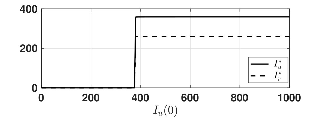 Figure 9
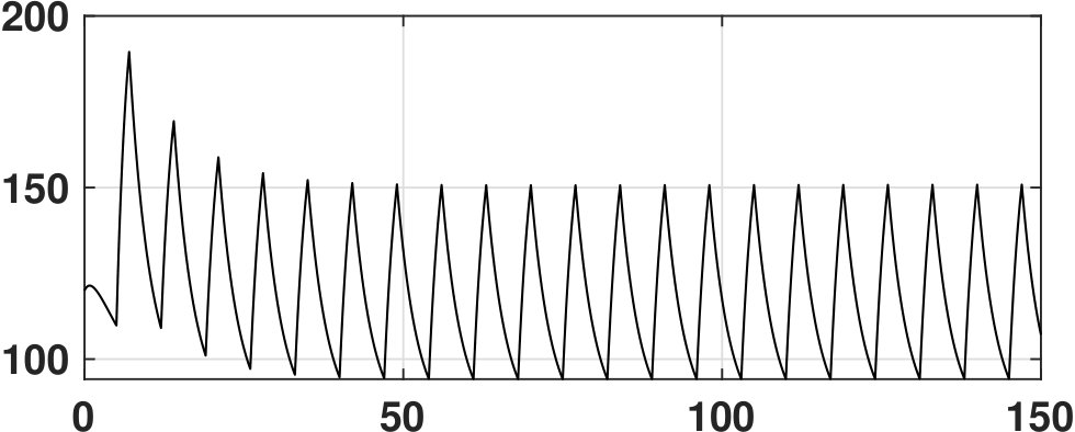 Figure 10
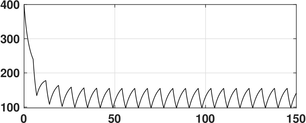 Figure 11
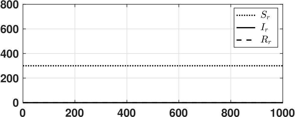 Figure 12
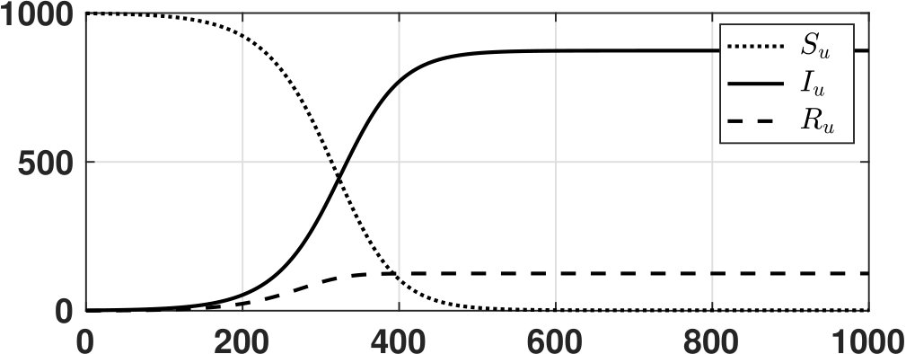 Figure 13
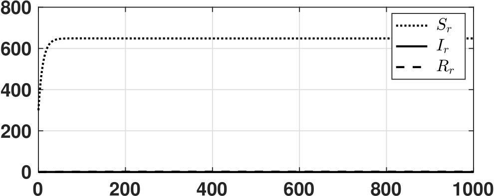 Figure 14
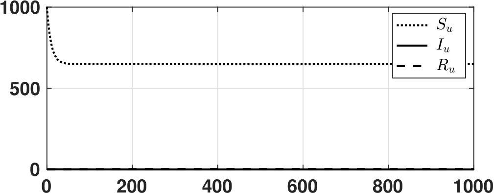 Figure 15
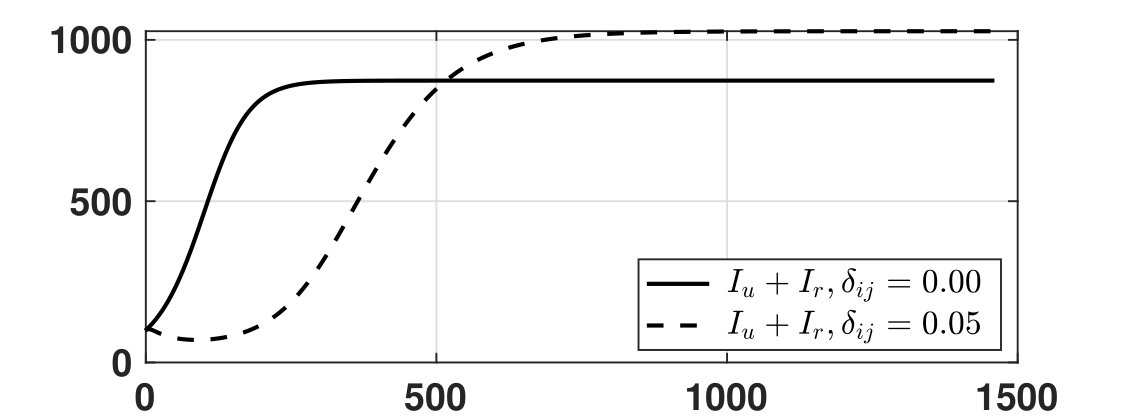 Figure 16
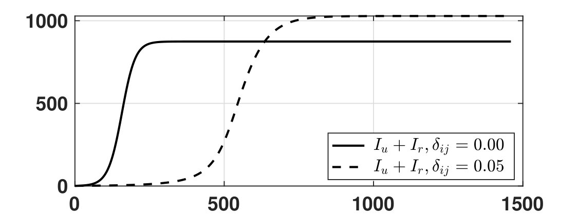 Figure 17
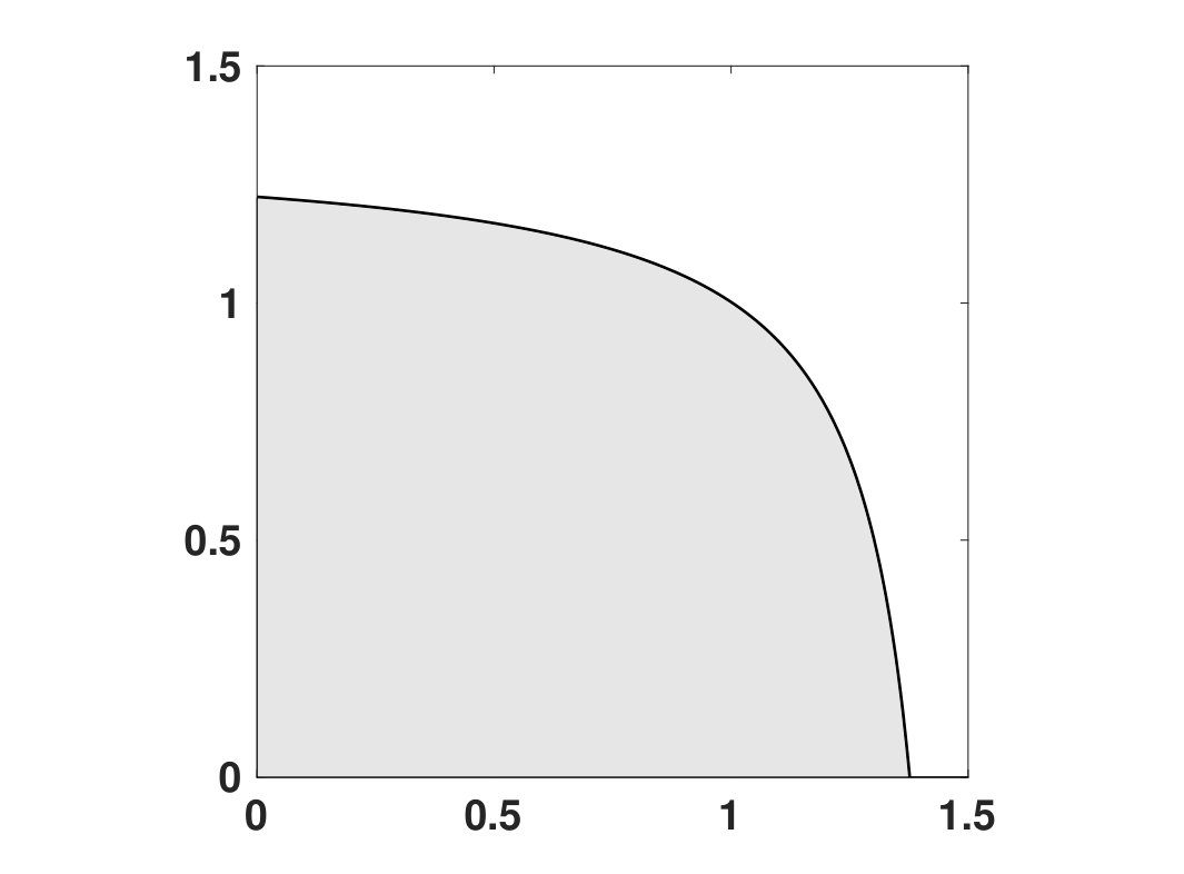 Figure 18
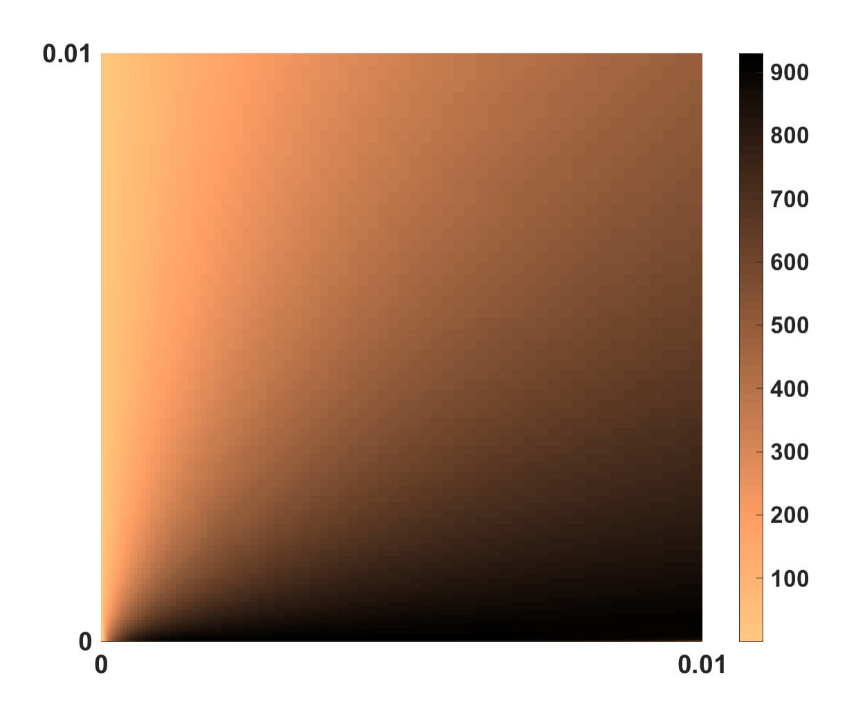 Figure 19
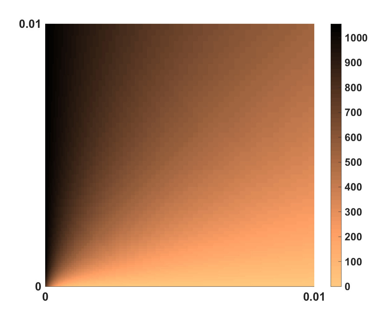 Figure 20
 Figure 21
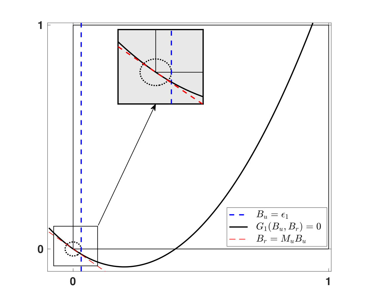 Figure 22
 Figure 23
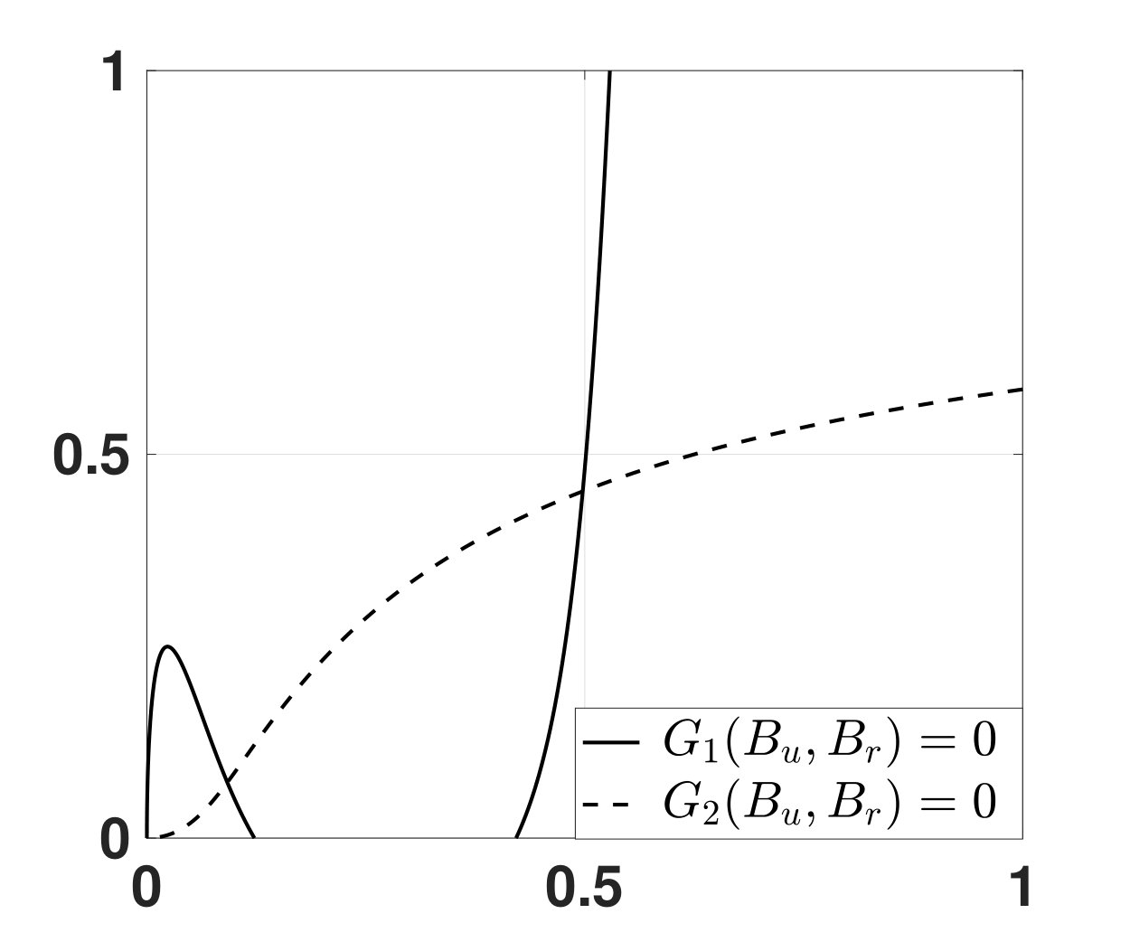 Figure 24
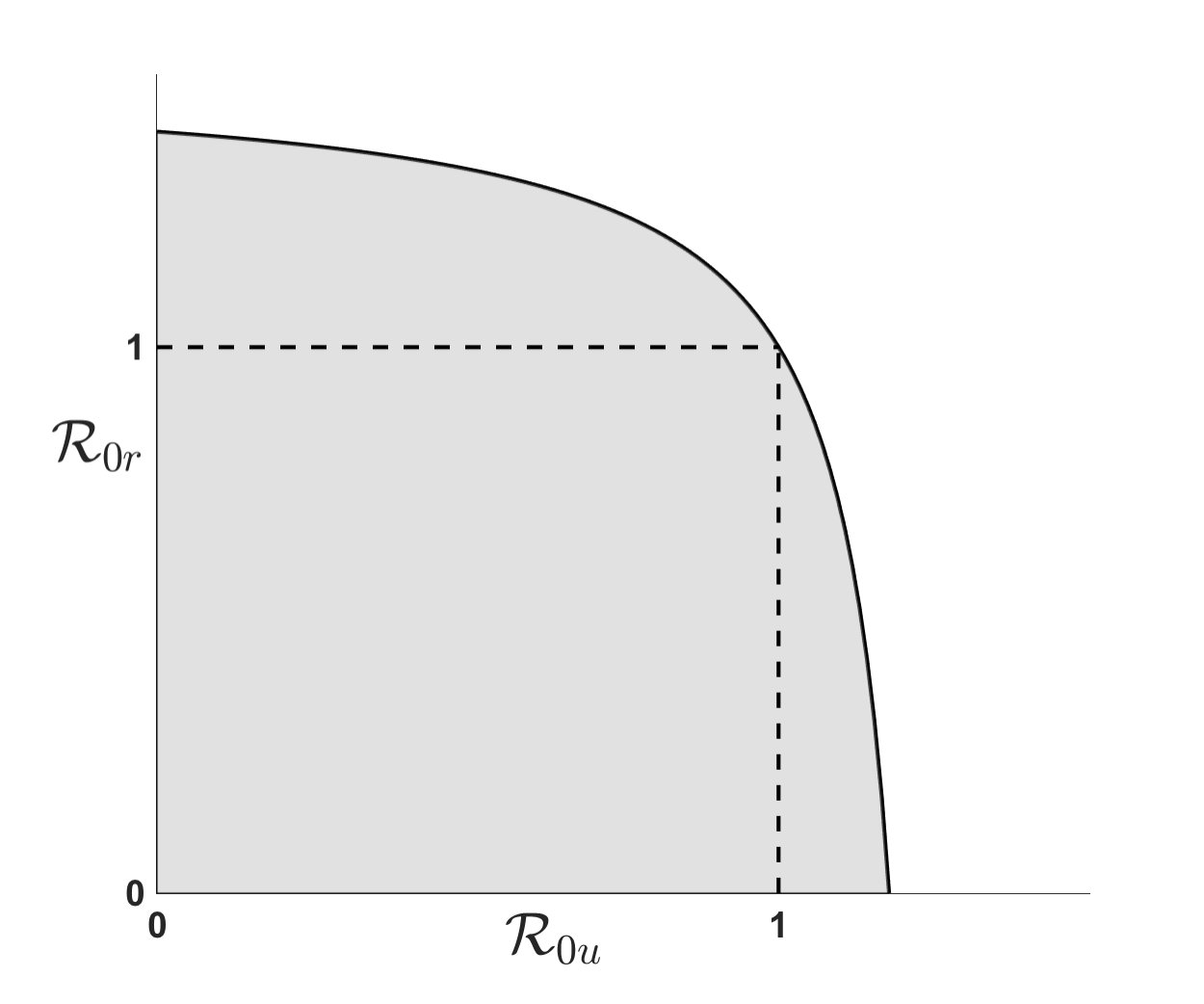 Figure 25
Peer Reviews
No public reviews on file for this paper yet. If you reviewed it on a platform where reviews are public (OpenReview, ICLR, NeurIPS, ICML), you can paste yours below so the community can read it here.
Videos
No videos yet. Explain this paper in a talk, walkthrough, or lecture? Add one.
\paginas
110
A two-patch epidemic model with nonlinear reinfection
Un modelo epidémico de dos poblaciones con reinfección no lineal
Juan G. Calvo CIMPA-Escuela de Matemática, Universidad de Costa Rica, San José, Costa Rica. E-Mail: [email protected]
Alberto Hernández CIMPA-Escuela de Matemática, Universidad de Costa Rica, San José, Costa Rica. E-Mail: [email protected]
Mason A. Porter Department of Mathematics, University of California Los Angeles, USA. E-Mail: [email protected]
Fabio Sanchez CIMPA-Escuela de Matemática, Universidad de Costa Rica, San José, Costa Rica. E-Mail: [email protected]
(Received: xx-xx-xx; Revised: xx-xx-xx;
Accepted: xx-xx-xx)
Abstract
The propagation of infectious diseases and its impact on individuals play a major role in disease dynamics, and it is important to incorporate population heterogeneity into efforts to study diseases. As a simplistic but illustrative example, we examine interactions between urban and rural populations in the dynamics of disease spreading. Using a compartmental framework of susceptible–infected–susceptible () dynamics with some level of immunity, we formulate a model that allows nonlinear reinfection. We investigate the effects of population movement in the simplest scenario: a case with two patches, which allows us to model movement between urban and rural areas. To study the dynamics of the system, we compute a basic reproduction number for each population (urban and rural). We also compute steady states, determine the local stability of the disease-free steady state, and identify conditions for the existence of endemic steady states. From our analysis and computational experiments, we illustrate that population movement plays an important role in disease dynamics. In some cases, it can be rather beneficial, as it can enlarge the region of stability of a disease-free steady state.
L
\KW
Dynamical systems; population dynamics; mathematical modeling; biological contagions; population movement.
a propagación de enfermedades infecciosas y su impacto en individuos juega un gran rol en la dinámica de la enfermedad, y es importante incorporar heterogeneidad en la población en los esfuerzos por estudiar enfermedades. De manera simplística pero ilustrativa, se examina interacciones entre una población urbana y una rural en la dinámica de la propagación de una enfermedad. Utilizando un sistema compartimental de dinámicas entres susceptibles–infectados–susceptibles () con cierto nivel de inmunidad, se formula un modelo que permite reinfecciones no lineales. Se investiga los efectos de movimiento de poblaciones en el escenario más simple: un caso con dos poblaciones, que permite modelar movimiento entre un área urbana y otra rural. Con el fin de estudiar la dinámica del sistema, se calcula el número básico reproductivo para cada comunidad (rural y urbana). Se calculan también puntos de equilibrio, la estabilidad local del estado libre de enfermedad, y se identifican condiciones para la existencia de estados de equilibrio endémicos. Del análisis y experimentos computacionales, se ilustra que el movimiento en la población jueva un rol importante en la dinámica del sistema. En algunos casos, puede ser beneficioso, pues incrementa la región de estabilidad del punto de equilibrio del estado libre de infección.
\PC
Sistemas dinamicos, dinámica de poblaciones; modelado matemático; contagios biológicos; movimiento de poblaciones.
\AMS
92D25, 92D30
1 Introduction
It is relatively easy for individuals to move between towns, cities, countries, and even continents; and incorporating movement between populations has become increasingly prevalent in the modeling and analysis of disease spreading [3, 22]. It is also important to consider movement in which individuals travel to a distinct location from their place of origin and then return to their original location in a relative short time. Such movement can lead to rapid spreading of infectious diseases, and examination of connected environments can give clues about the types of strategies that are needed for control of disease propagation [2, 19].
In 2003, the Severe Acute Respiratory Syndrome (SARS) epidemic was a major concern among public health officials worldwide [4]. This new infectious disease spread rapidly, and scientists and researchers scrambled to try to discern how to contain its spread (e.g., by reducing the spreading rate) and to seek treatments and a vaccine. The best control measure that was found at the time was to isolate individuals who had been in contact with infected individuals. The rapid spread of the disease was associated with movement of a doctor who was identified as “Patient 0” for SARS [8, 23]. Population movement has also played an important role in subsequent events, such as the spread of ebola to the western hemisphere [5], the spread of measles in some parts of the world by travelers [6], and the resurgence of malaria through the massive migration of Nicaraguans to the northern part of Costa Rica [1].
The use of compartmental models to describe the spreading of diseases has been explored thoroughly in numerous scenarios [3, 22]. For example, when there is nonlinear reinfection, an individual who was infected previously can become infected again through contact with an infectious individual after losing immunity [15]. Several models that allow individuals to lose immunity and become infectious again also exhibit a backward bifurcation in which a stable endemic equilibrium coexists with a stable disease-free equilibrium when the associated basic reproduction number is smaller than [11, 24, 27, 28, 26]. Moreover, in social contagion processes (e.g., spread of use of drugs, adoption of products, and so on), after an initial “contagion”, some models include a backward bifurcation that can arise via social inputs [27].
In the present paper, we generalize the compartmental model from [24], who studied a continuous dynamical system (in the form of coupled ordinary differential equations) that describes interactions between susceptible and infected individuals with the possibility of reinfection after loss of immunity, by incorporating population movement between urban and rural environments. Taking population movement into account is important for studies of disease dynamics in practice, and it changes the qualitative dynamics of disease spreading. We explore the simplest case, in which a population has two patches, and yield insights that will be useful for later explorations of disease spreading in a population that includes a network of patches.
Our paper proceeds as follows. In Section 2, we describe our compartment model of disease spreading (including nonlinear reinfection) between urban and rural environments. In Section 3, we give a formula for the model’s basic reproduction number , analyze the existence and local stability of the disease-free state, and study the existence of endemic equilibria. In Section 4, we illustrate several example scenarios with numerical computations. Finally, in Section 5, we conclude and discuss the biological insights of our model.
2 A two-patch compartmental model
We present a two-patch model of disease spreading in humans that incorporates nonlinear reinfection and population movement. Specifically, we generalize the model by Sanchez et al. [24] by incorporating the idea of urban versus rural environments. We use the subscript for urban variables and parameters and the subscript for rural variables and parameters. For , let , , and denote the numbers of susceptible, infected, and post-recovery susceptible individuals, respectively. New susceptible individuals enter the system in proportion to the total population , where . Let denote the rate of both births and deaths (for simplicity, we assume that they are the same.) Susceptible individuals become infected at a rate of , infected individuals transition to a state of post-recovery susceptibility at a rate of , and post-recovery susceptible individuals can be reinfected at a rate of . Such reinfection corresponds to infectious diseases (such as tuberculosis, malaria, and others [13, 14]) in which subsequent infections are possible after loss of immunity. Typically, when there exists the possibility of reinfection, an initial infection tends to produce stronger symptoms [21]. We model movement between patches using the functions , which denote the fraction of individuals who travel from patch to patch (with ) at time .
Our model consists of the following coupled system of ordinary differential equations:
[TABLE]
with initial conditions , , and (for ).
By adding the first three and last three equations in (1), we see that and satisfy the linear dynamical system
[TABLE]
Its solution is
[TABLE]
where is the net movement of individuals at time . The initial conditions are and .
In our analysis, we assume at first that and are constant, such that and simplify to
[TABLE]
There are three cases:
There is no movement (i.e., ), which corresponds to the case of independent patches that was studied in [24]. In this case, each patch has a backward bifurcation, and the steady state can depend on the number of initially infected individuals. 2. 2.
Movement occurs exclusively from one patch to the other. For example, suppose that and . In this case, (i.e., eventually, the entire population is in ). There is a backward bifurcation in this case as well, but now there is a total population of in the urban patch. We explore this case in Example 4.1 in Section 4. 3. 3.
There is movement in both directions between the two patches (i.e., and ). This is the primary scenario (and the principal novel contribution) of the present paper.
3 Analysis of our model
3.1 Disease-free steady state and basic reproduction number
Because the total population is constant, we can eliminate from the dynamical system (1). We then compute the Jacobian matrix of (1) and evaluate it at the disease-free steady state
[TABLE]
to obtain the matrix
[TABLE]
where and . For the dynamical system (1), equilibria with necessarily also satisfy .
The five eigenvalues of the matrix (3) are
[TABLE]
All eigenvalues are real, and and are negative. The two remaining eigenvalues are negative as long as
[TABLE]
When there is only one population (i.e., one patch), the basic reproduction number is . For our multiple-patch case, we define a “local basic reproduction number” for each patch:
[TABLE]
We can then express the conditions in (4) as
[TABLE]
See Figure 1 for an illustration of a typical region in which all eigenvalues are negative. For progressively smaller and , the shaded region approaches the unit square.
We have thus established the following lemma.
Lemma 3.1
Assume that Eqs. (5) hold. It then follows that the disease-free steady state (2) of the dynamical system (1) is locally asymptotically stable.
Remark 3.2
The conditions in (5) are satisfied when and . We then have local stability in the rural and urban patches if we treat them as independent. Additionally, from Lemma 3.1, we see that it is possible to obtain local asymptotic stability for the disease-free steady state (2) even when one or both local basic reproduction numbers are larger than . In such a scenario, movement is beneficial, as it leads to local asymptotic stability of the disease-free steady state in situations that would not be the case for independent patches. We illustrate such a scenario in Example 4.2 in Section 4. **
3.2 Technical tool: The Poincaré–Miranda theorem
As preparation for analyzing the existence of steady states in our model, we briefly recall some classical results by Poincaré and others. See [12, 16, 30, 31] for detailed accounts of the relevant theory. In 1817, Bolzano proved the following well-known theorem:
Theorem 3.3
Let be a continuous function such that . There then exists such that .
Definition 3.4
Let , and let denote its boundary. For each , let
[TABLE]
be the opposite -th faces of the boundary .
In 1883–1884, Poincaré announced a generalization of Bolzano’s theorem without providing a proof.
Theorem 3.5** (Poincaré)**
Let , with , be a continuous map such that
[TABLE]
and
[TABLE]
for every . It then follows that there exists such that .
In the 1940s, Miranda rediscovered Poincaré’s theorem and showed that it is logically equivalent to Brower’s fixed-point theorem. Since then, this result has often been called the Poincaré–Miranda theorem. We require a modified version of the Poincaré–Miranda theorem in two dimensions.
Proposition 3.6
Let such that is continuous and . Assume that
[TABLE]
Assume additionally that and are both continuous from the right at , with and . It then follows that there exists such that .
Proof 3.7**.**
Because is continuous, both and are also continuous. Using the facts that for all and that is continuous from the right, it follows that there exists such that for all . By the implicit function theorem, for , one can write , where the function is differentiable. Therefore,
[TABLE]
By the continuity of in the compact set and using Equation (6), it follows that there exists such that for all . By the same argument, there also exists such that for all . By the Poincaré–Miranda theorem, there must exist such that .
3.3 Existence of multiple-population endemic steady states
We now examine endemic steady states, in which there are infected individuals at steady state in both the urban and rural patches.
We start by proving the following lemma.
Lemma 3.8**.**
Suppose that and . It then follows that exists at least one endemic state, for which both and . This is, there are infected individuals at steady state in both the urban and the rural patches.
Proof 3.9**.**
We deduce the existence of a solution of the following nonlinear system of algebraic equations:
[TABLE]
Given two parameters , we consider the auxiliary linear system
[TABLE]
Suppose that is a solution of the linear system (8). This solution also satisfies the nonlinear system (7) if and . By adding all of the equations in (8), we see that . We then rescale variables in (8) by substituting
[TABLE]
to obtain a linear system of algebraic equations with parameters and . This system is
[TABLE]
We now solve Eqs. (9a) and (9d) to obtain
[TABLE]
Using Eqs. (9b), (9c), (9e), (9f), we solve for and to obtain
[TABLE]
where
[TABLE]
One can write similar expressions for and . The solution of (9) satisfies the nonlinear algebraic system (7) if and only if and . We then define
[TABLE]
We will show that the system
[TABLE]
has at least one solution . This implies the existence of a solution of the nonlinear algebraic system (7) with and . This solution corresponds to a steady state with a nonzero infected population in both the urban and the rural patches.
Consider the surface . We have that for , with equality when . Because , we need to cut the origin to guarantee the existence of a positive solution of Eq. (10). A straightforward calculation yields
[TABLE]
because by hypothesis. Analogously, we compute that
[TABLE]
We also compute that for and that for . By Proposition 3.6, we conclude that there exists such that . Therefore, the nonlinear algebraic system (7) has a solution that corresponds to a steady state with positive values for both and .
Remark 3.10**.**
Using numerical computations, we can observe the existence of two or more distinct endemic steady states. However, we need to explore them further to characterize them; see Figure 2b and Examples 4.3 and 4.7 in Section 4. **
4 Examples
We now present some numerical simulations of the dynamical system (1) for a variety of parameter values. Using these examples, we illustrate that population movement strongly influences how a disease can propagate.
Example 4.1**.**
We first explore the behavior of our model (1) when and , which describes movement in one direction (specifically, from the rural patch to the urban one). In some countries, it is common for individuals in rural areas to move to urban areas for work [7]. This is a type of short-term mobility. We consider the following parameter values:
[TABLE]
with initial conditions
[TABLE]
In this case,
[TABLE]
In Figure 3, we show as we vary . We show the solutions for both the urban and the rural patches when (i.e., when there is no movement) and in Figure 4. We observe that movement in one direction increases the number of infected individuals and that larger values of affects only the approach speed to the steady state.
Example 4.2**.**
We now compare the effects of conditions (5a) and (5b) to the standard condition for local asymptotic stability of the disease-free steady state (2). We use the parameter values
[TABLE]
and initial conditions
[TABLE]
We calculate that and . Therefore, in the absence of movement, disease persists in the urban patch but dies out in the rural patch; see Figures 5a and 5b. For , we calculate that , so conditions (5) are satisfied. Therefore, the disease-free steady state is locally asymptotically stable; see Figures 5c and 5d.
In this example, there exists one endemic state, with . We study two variations:
- (1)
When the initial number of infected individuals increases, we reach the endemic steady state. See Figure 6a for an illustration with initial conditions and . 2. (2)
When we slightly increase to , condition (5c) is no longer satisfied, and the system has an endemic state with just one initial infected individual in the urban patch; see Figure 6b.
Example 4.3**.**
We now give an example with two endemic states. We use the parameter values
[TABLE]
We fix the initial conditions
[TABLE]
and vary the initial number of infected individuals in the urban patch from [math] to . In this case, there are two endemic states, with and , which we illustrate in Figure 2b. We show and as a function of in Figure 7. We observe that the steady state is unstable.
Example 4.4**.**
In this example, we explore the dependence on and in our model to illustrate the region of local asymptotic stability from Eqs. (5). We consider the parameter values
[TABLE]
We fix the initial conditions
[TABLE]
and vary and ; see our results in Figure 8. We observe that the conditions in Eqs. (5) precisely describe the disease-free region (in gray). Therefore, or can have a value that is slightly larger than in situations with a disease-free steady state. This is not the case when we consider just one patch, so movement can be beneficial.
Example 4.5**.**
In this example, we study how a disease spreads through the two populations as we vary and when initially one infected person arrives at one patch. We consider the parameter values
[TABLE]
We fix the initial conditions
[TABLE]
and vary and . We show our results in Figure 9.
Example 4.6**.**
To model different rates of movement between patches on weekdays and weekends, we now take and to be piecewise constant and periodic. Specifically, we take and as in Figure 10. In Figure 11, we show the results of our numerical computations using the parameter values
[TABLE]
with initial conditions
[TABLE]
Example 4.7**.**
We now revisit Remark 3.10, where we stated that we can observe numerically the existence of several distinct endemic steady states. Equation (10) is equivalent to a polynomial equation (as a function of or of degree , for which there can exist solutions (for or ). For the parameter values
[TABLE]
we see that all solutions are in the interval . They correspond to feasible steady states ; see Figure 12. We see numerically that of these points are locally stable.
5 Conclusions and Discussion
The dynamics of spreading diseases are influenced significantly by spatial heterogeneity and population movement. In this paper, we illustrated the importance of incorporating movement into models of disease dynamics using a simple but biologically meaningful model. Specifically, we constructed a two-patch compartmental model that incorporates movement between urban and rural populations, as well as the possibility of reinfection after recovery.
When there is a lot of population movement, there are regions of local asymptotic stability of the disease-free steady-state even when the basic reproduction number . This arises predominantly from the numerous individuals who move between patches.
The exploration of interacting populations plays an important role in the understanding of disease dynamics. Many models of disease spreading focus on a single population [3], but populations do not exist in isolation. Using our two-patch model with urban and rural environments, we illustrated several examples of plausible real-world scenarios in which movement yields insightful information about disease spreading and epidemics. We expect that such dynamics will be relevant for studies of disease spreading on networks, such as when many people commute daily between their homes in rural areas and work in urban centers (as is the case in many countries in South and Central America).
6 Acknowledgements
We thank the Research Center in Pure and Applied Mathematics and the Mathematics Department at Universidad de Costa Rica for their support during the preparation of this manuscript. The authors gratefully acknowledge institutional support for project B8747 from an UCREA grant from the Vice Rectory for Research at Universidad de Costa Rica. We also acknowledge helpful discussions with Prof. Luis Barboza, Prof. Carlos Castillo-Chavez, and Prof. Esteban Segura.
The reference list from the paper itself. Each links out to its DOI / PubMed record.
- 1[1] Alvarado, L. (2018) “Costa Rica Once Again Under Malaria Alert”, in https://news.co.cr/costa-rica-once-again-under-malaria-alert/73681 , accessed 25/04/2019.
- 2[2] Bichara, D.; Castillo-Chavez, C. (2016) “Vector-borne diseases models with residence times — A Lagrangian perspective”, Math. Biosci. 281 :128–138.
- 3[3] Brauer, R.; Castillo-Chavez, C. (2012) Mathematical Models in Population Biology and Epidemiology , 2nd edition, Springer-Verlag (Providence, RI, USA).
- 4[4] Center for Disease Control and Prevention: Severe Acute Respiratory System (SARS) , 2019. Available from: https://www.cdc.gov/sars/index.html .
- 5[5] Center for Disease Control and Prevention: Ebola (Ebola Virus Disease) , 2019. Available from: https://www.cdc.gov/vhf/ebola/history/2014-2016-outbreak/index.html#anchor_1515001446180
- 6[6] Center for Disease Control and Prevention: Measles (Rubeola) , 2019. Available from: https://www.cdc.gov/measles/index.html .
- 7[7] Coffee, M.P.; Garnett, G.P.; Mlilo, M.; Voeten, H.A.C.M.; Chandiwana, S.; Gregson, S. (2005) “Patterns of Movement and Risk of HIV Infection in Rural Zimbabwe”, J. Infect. Dis. 191 (1):S 159–S 167.
- 8[8] Chowell G.; Fenimore P.W.; Castillo-Garsow M.A.; Castillo-Chavez C. (2004) “SARS outbreaks in Ontario, Hong Kong and Singapore: The role of diagnosis and isolation as a control mechanism”, J. Theor. Biol. 224 (1):1–8.