Interpolation and extrapolation of global potential energy surfaces for polyatomic systems by Gaussian processes with composite kernels
Jun Dai, Roman V. Krems

TL;DR
This paper introduces an improved Gaussian process approach with composite kernels for accurately modeling global potential energy surfaces of polyatomic molecules, enabling effective interpolation and extrapolation with fewer data points.
Contribution
The study presents an automated kernel selection method, iterative kernel complexity enhancement, and demonstrates physical extrapolation of PES using Gaussian processes with composite kernels.
Findings
Achieved 65.8 cm$^{-1}$ RMS error with 500 points for H$_3$O$^+$ PES.
Extended PES accuracy to 21,000 cm$^{-1}$ using only low-energy points.
Validated PES extrapolation at high energies based on low-energy data.
Abstract
Gaussian process regression has recently emerged as a powerful, system-agnostic tool for building global potential energy surfaces (PES) of polyatomic molecules. While the accuracy of GP models of PES increases with the number of potential energy points, so does the numerical difficulty of training and evaluating GP models. Here, we demonstrate an approach to improve the accuracy of global PES without increasing the number of energy points. The present work reports four important results. First, we show that the selection of the best kernel function for GP models of PES can be automated using the Bayesian information criterion as a model selection metric. Second, we demonstrate that GP models of PES trained by a small number of energy points can be significantly improved by iteratively increasing the complexity of GP kernels. The composite kernels thus obtained maximize the accuracy of…
Click any figure to enlarge with its caption.
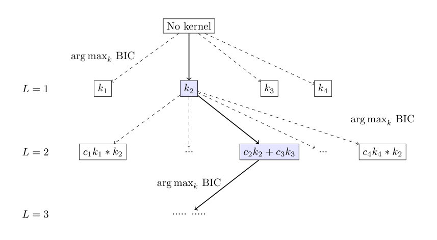 Figure 1
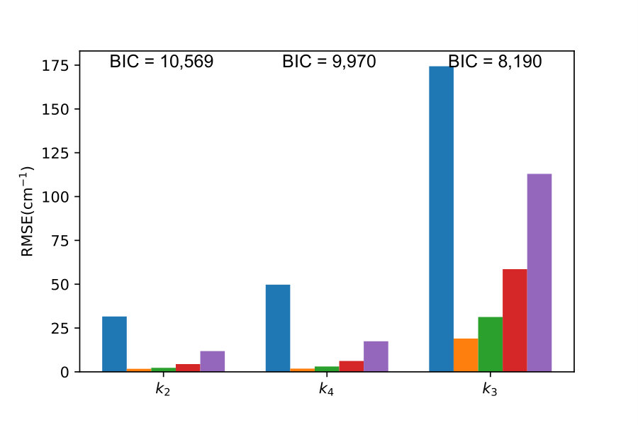 Figure 2
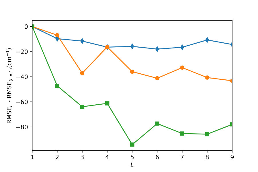 Figure 3
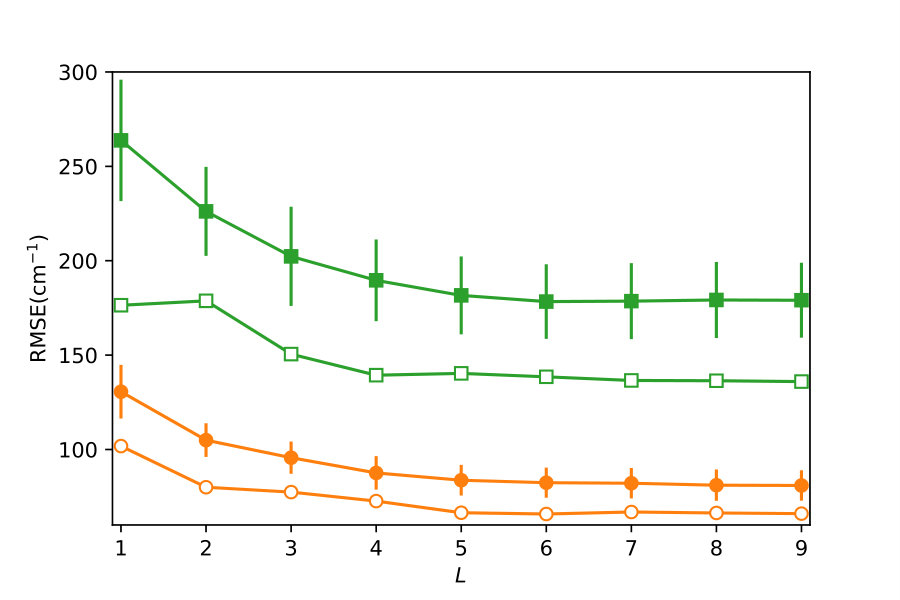 Figure 3
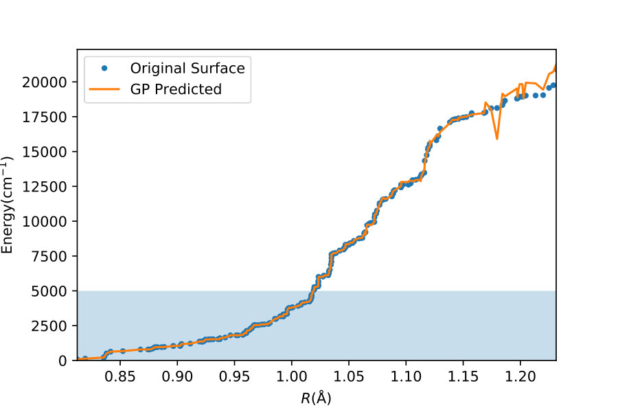 Figure 4
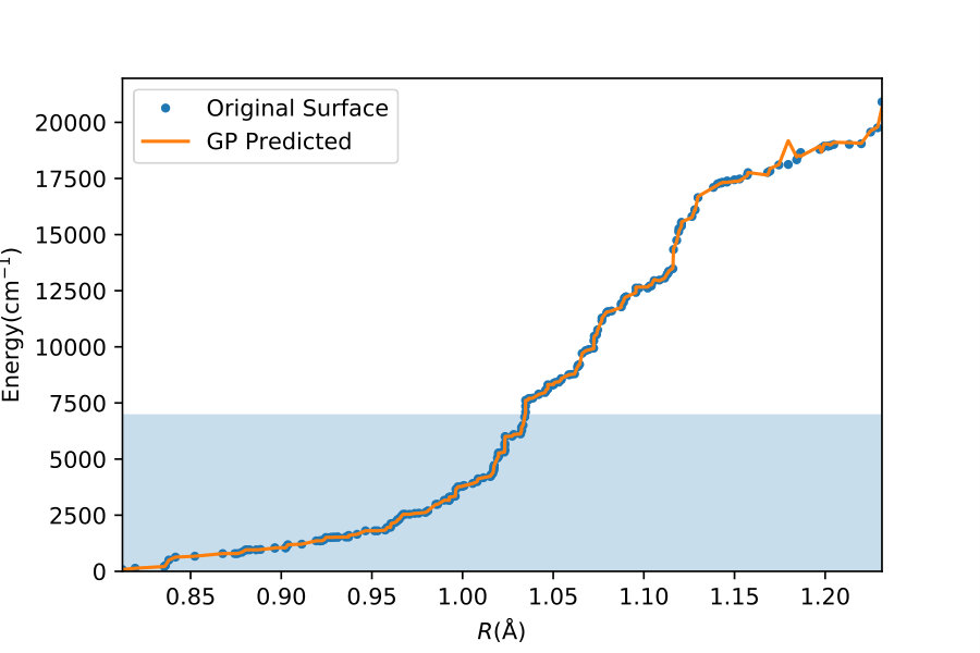 Figure 4
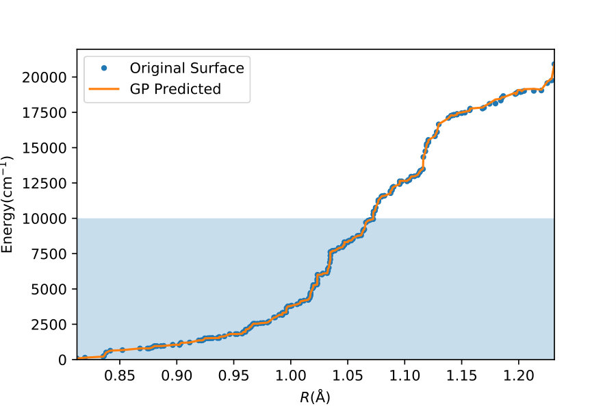 Figure 4
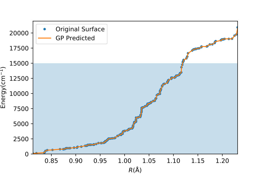 Figure 4
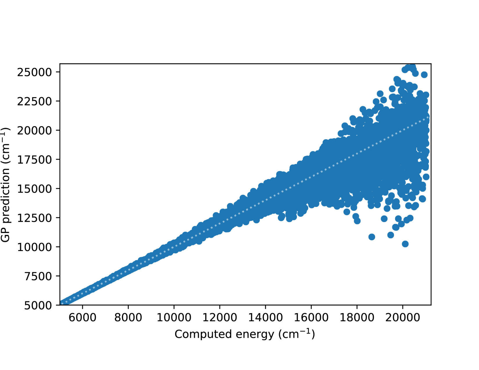 Figure 5
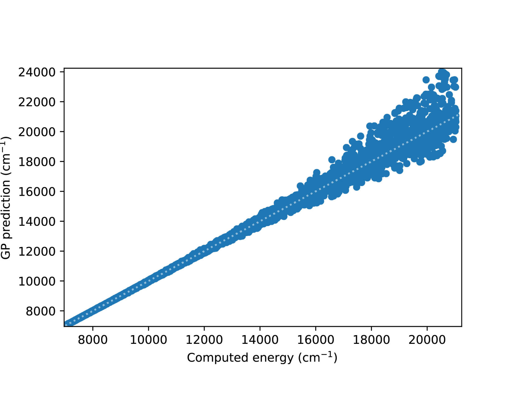 Figure 5
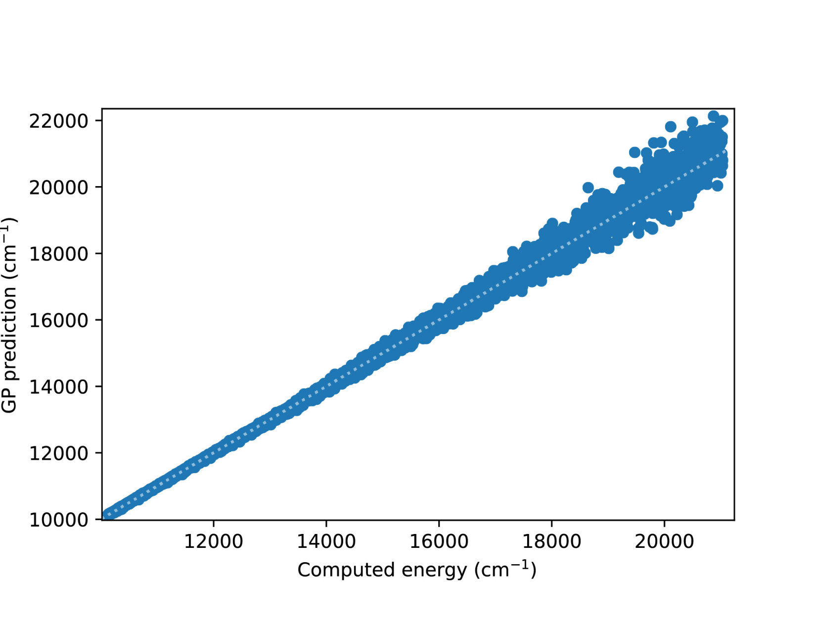 Figure 5
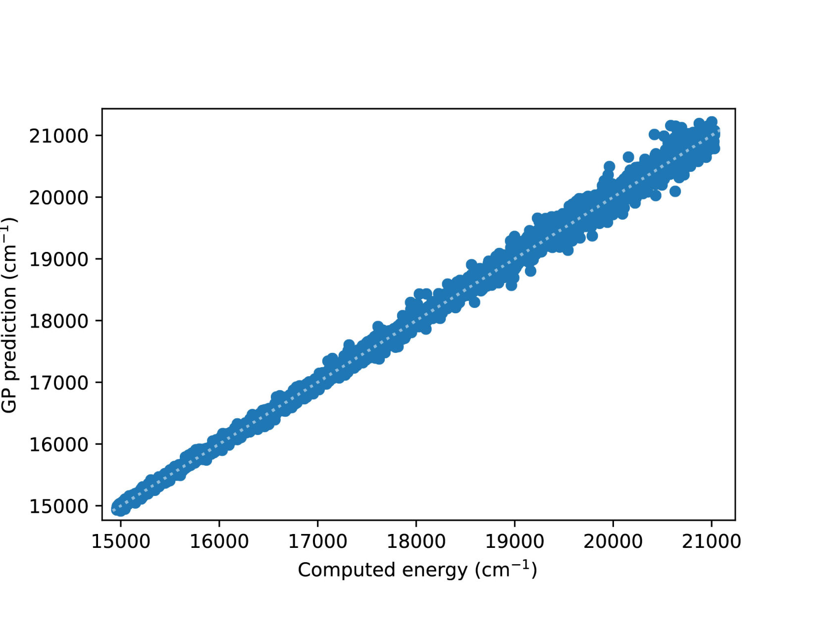 Figure 5
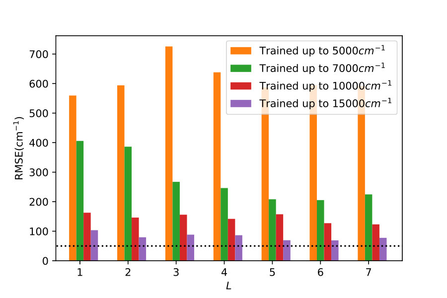 Figure 6
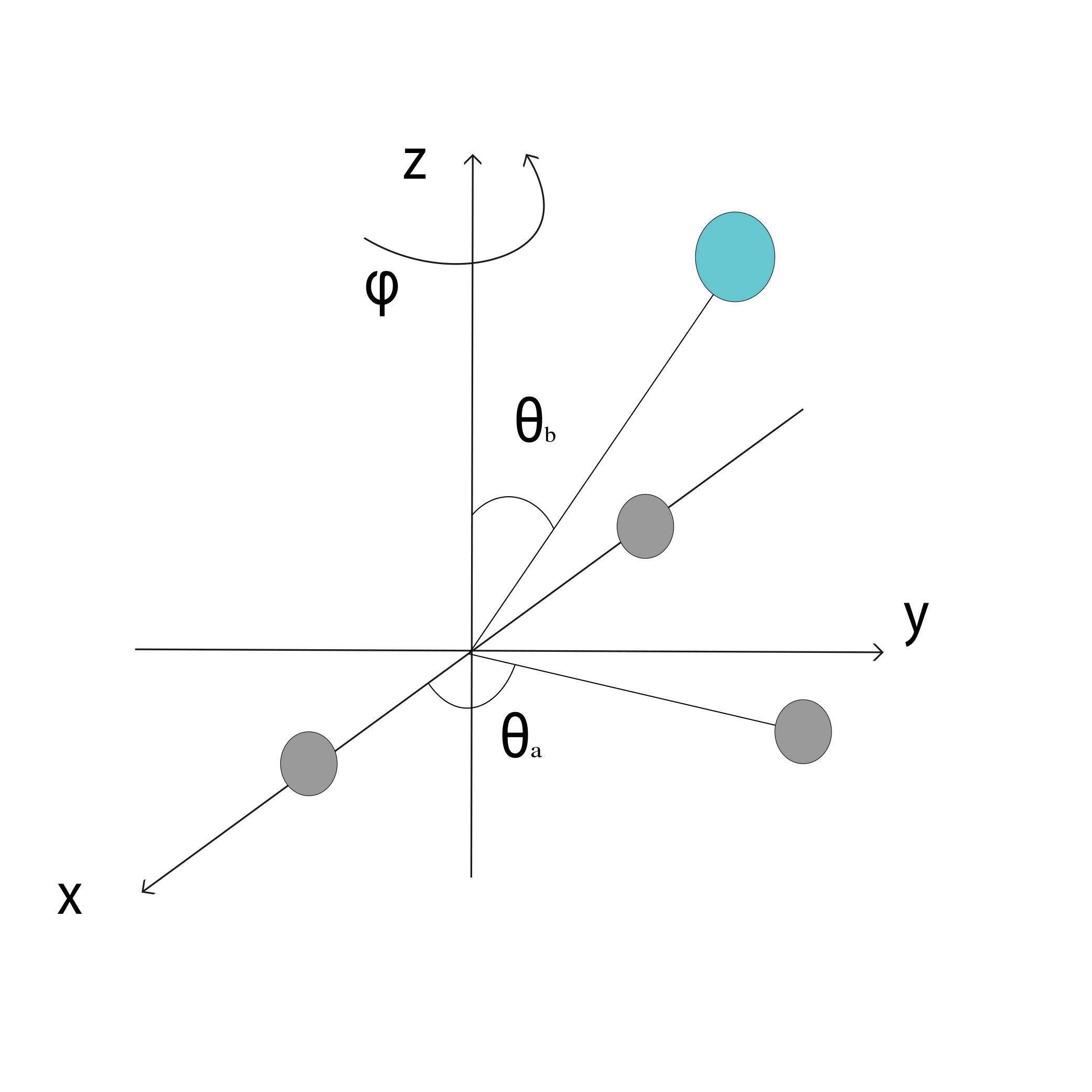 Figure 7
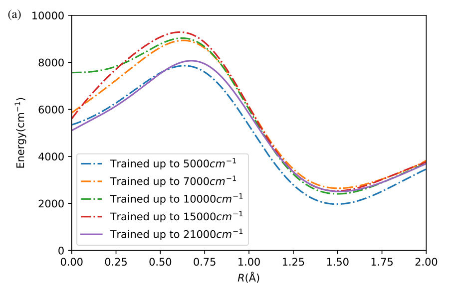 Figure 8
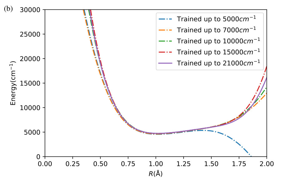 Figure 8
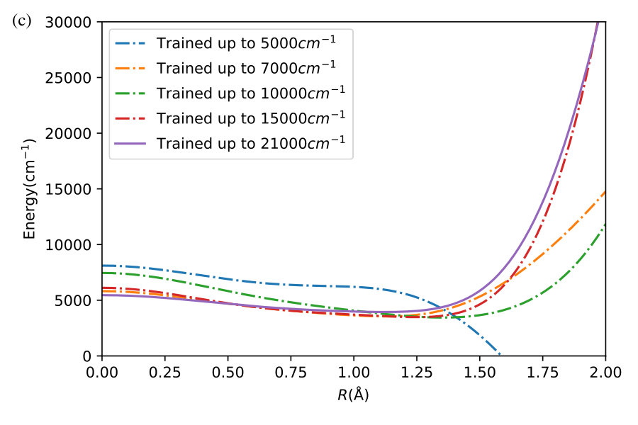 Figure 8
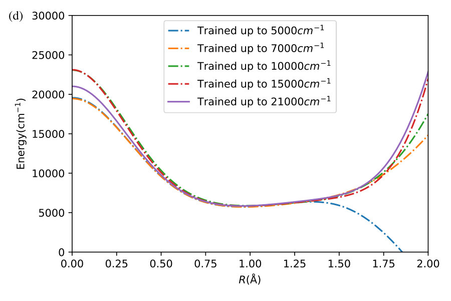 Figure 8
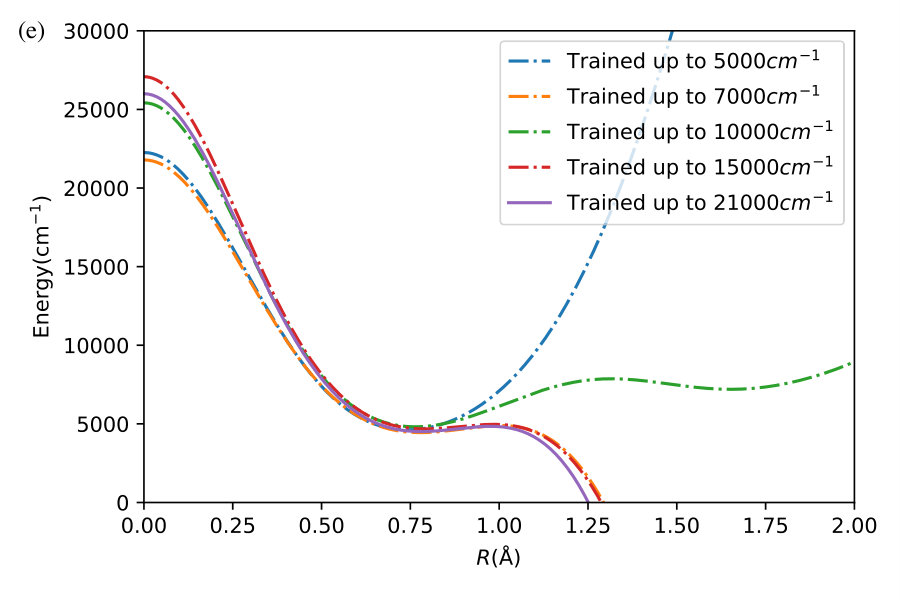 Figure 8
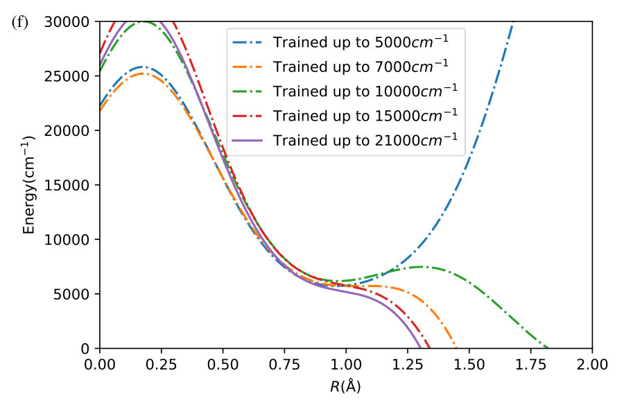 Figure 8
Peer Reviews
No public reviews on file for this paper yet. If you reviewed it on a platform where reviews are public (OpenReview, ICLR, NeurIPS, ICML), you can paste yours below so the community can read it here.
Videos
No videos yet. Explain this paper in a talk, walkthrough, or lecture? Add one.
Taxonomy
TopicsMachine Learning in Materials Science · Computational Drug Discovery Methods · Protein Structure and Dynamics
Interpolation and extrapolation of global potential energy surfaces for polyatomic systems
by Gaussian processes with composite kernels
J. Dai and R. V. Krems
Department of Chemistry, University of British Columbia, Vancouver, B.C. V6T 1Z1, Canada
Abstract
Gaussian process regression has recently emerged as a powerful, system-agnostic tool for building global potential energy surfaces (PES) of polyatomic molecules. While the accuracy of GP models of PES increases with the number of potential energy points, so does the numerical difficulty of training and evaluating GP models. Here, we demonstrate an approach to improve the accuracy of global PES without increasing the number of energy points. The present work reports four important results. First, we show that the selection of the best kernel function for GP models of PES can be automated using the Bayesian information criterion as a model selection metric. Second, we demonstrate that GP models of PES trained by a small number of energy points can be significantly improved by iteratively increasing the complexity of GP kernels. The composite kernels thus obtained maximize the accuracy of GP models for a given distribution of potential energy points. Third, we show that the accuracy of the GP models of PES with composite kernels can be further improved by varying the training point distributions. Fourth, we show that GP models with composite kernels can be used for physical extrapolation of PES. We illustrate the approach by constructing the six-dimensional PES for H3O+. For the interpolation problem, we show that this algorithm produces a global six-dimensional PES for H3O+ in the energy range between zero and cm*-1* with the root mean square error cm*-1* using only 500 randomly selected ab initio points as input. To illustrate extrapolation, we produce the PES at high energies using the energy points at low energies as input. We show that one can obtain an accurate global fit of the PES extending to cm*-1* based on 1500 potential energy points at energies below cm*-1*.
I Introduction
Quantum properties of polyatomic molecules are computed by solving the nuclear Schrödinger equation that is parametrized by potential energy surfaces (PES). These PES are generally obtained by fitting the results of the electronic structure calculations at different points of the nuclear configuration space. Many different techniques have been developed for fitting multi-dimensional PES (for representative examples, see Refs. fitting-PES ; general-fitting-1 ; general-fitting-2 ; general-fitting-4 ; general-fitting-5 ; BML ). A major thrust of recent research has been to develop approaches for fitting PES of polyatomic systems by machine learning (ML) models ML-for-PES ; NNs-for-PES ; NNs-for-PESa ; NNs-for-PES-1a ; NNs-for-PES-1b ; NNs-for-PES-1c ; NNs-for-PES-2 ; NNs-for-PES-3 ; NNs-for-PES-4 ; NNs-for-PES-5 ; NNs-for-PES-6 ; gp-1 ; gp-2 ; gp-3 ; jie-jpb ; gp-for-PES-2 ; gp-for-PES-3 ; gp-for-PES-4 ; gp-for-PES-5 ; gp-for-PES-6 ; gp-for-PES-7 ; gp-for-PES-8 ; gp-for-PES-9 ; gp-for-PES-10 . These models can be classified into approaches using artificial neural networks (NNs) ML-for-PES ; NNs-for-PES ; NNs-for-PESa ; NNs-for-PES-1a ; NNs-for-PES-1b ; NNs-for-PES-1c ; NNs-for-PES-2 ; NNs-for-PES-3 ; NNs-for-PES-4 ; NNs-for-PES-5 ; NNs-for-PES-6 and methods based on kernels general-fitting-2 ; BML ; rabitz-1 ; rabitz-2 ; rabitz-3 , such as kernel ridge regression or Gaussian process regression gp-1 ; gp-2 ; gp-3 ; jie-jpb ; gp-for-PES-2 ; gp-for-PES-3 ; gp-for-PES-4 ; gp-for-PES-5 ; gp-for-PES-6 ; gp-for-PES-7 ; gp-for-PES-8 ; gp-for-PES-9 ; gp-for-PES-10 . ML models have become popular because (i) they provide flexible representations of PES that can potentially be applied to molecular systems of any complexity; (ii) they are easy to construct given the abundance of relevant packages readily available.
The NN and kernel-based models of PES are generally designed to make accurate predictions of the potential energy within the range of the given potential energy points. NNs achieve this by an analytical fit of the given points, while kernel-based methods interpolate the given points. However, the accuracy and numerical complexity of quantum chemistry calculations depends on the geometry of a given polyatomic system. For example, it is much more difficult to compute the potential energy at large intermolecular separations or where multiple electronic states exhibit degeneracies. At the same time, for complex molecular systems, the specific features of the PES in different parts of the configuration space are not a priori known. Therefore, for complex molecules, it is not generally known how to ensure that all important features of the PES fall within the range of the electronic structure calculations. An illustrative example of this challenge is the PES for the collision system of two alkali metal molecules nak , of importance to ultracold chemistry experiments my-book . For such and more complex molecular systems, it would be desirable to develop ML approaches that could construct PES by extrapolation of a small number of ab initio points randomly placed in the configuration space. Such models of PES could be used to explore the entire landscape of the PES and inform further ab initio calculations to generate flexible and highly accurate PES for complex systems. At present, there is no general procedure for building global PES by extrapolation. For example, if the PES is known only at low energies, it is generally considered unfeasible to build a global PES that is accurate at high energies in the entire configuration space. One of the goals of the present work is to demonstrate the feasibility of building ML models of PES by extrapolation.
The focus of the present work is on GP regression. While NNs provide parametric models of PES, GP models are nonparamteric. A nonparametric model can be viewed as one with an infinite number of parameters, whose distributions are adjusted in response to given potential energy points BML in order to yield an accurate representation of a PES, on average. Using GPs to construct PES for polyatomic systems has several advantages over other methods BML . First, it has been shown that accurate GP models can be obtained with a much smaller number of potential energy points than required for any other fitting method jie-jpb ; gp-for-PES-4 . Second, the construction of the models does not require any knowledge of the functional form of the PES and is completely automated. The same code can be applied to the construction of PES for different molecules of different complexity. This makes GP models ideal for applications aiming to invert the scattering problem rodrigo-bo or where the PES is iteratively improved by adding more ab initio calculations to relevant parts of the configuration space. Finally, there is no effort required to control overfitting in GP models of PES, at least, for systems with less than 15 degrees of freedom that have been fitted with GP models in the literature so far jie-jpb ; gp-for-PES-2 ; gp-for-PES-3 ; gp-for-PES-4 ; gp-for-PES-5 ; gp-for-PES-6 ; gp-for-PES-7 ; gp-for-PES-8 ; gp-for-PES-9 ; gp-for-PES-10 .
The present work reports several significant results. We first consider the interpolation problem, as in previous work gp-1 ; gp-2 ; gp-3 ; jie-jpb ; gp-for-PES-2 ; gp-for-PES-3 ; gp-for-PES-4 ; gp-for-PES-5 ; gp-for-PES-6 ; gp-for-PES-7 ; gp-for-PES-8 ; gp-for-PES-9 ; gp-for-PES-10 , and show that the accuracy of the resulting GP models of the PES can be significantly enhanced by increasing the complexity of GP model kernels. All previous authors considered GP models of PES with simple, fixed kernels. The accuracy of such models was increased by increasing the number of potential energy points. However, the numerical difficulty of training a GP model scales with the number of potential energy points as and the evaluation time of a GP model, once trained, scales as . It is therefore necessary to develop approaches that produce more accurate GP models with smaller . The present work demonstrates an interpolation approach that can be used to enhance the accuracy of the PES model with a fixed number of energy points by building composite kernels with increased complexity. In particular, we propose an algorithm to enhance the accuracy of the PES through optimization in the space of kernels by varying random distributions of ab initio points with fixed . Our final result illustrates that GP models of PES for polyatomic systems can be constructed to be accurate both within and outside the range of the given potential energy points.
This work builds on the demonstration that the predictive power of GP models can be enhanced by increasing the kernel complexity using the Bayesian information criterion (BIC) as a metric extrapolation-1 ; extrapolation-2 ; extrapolation-3 . The kernel selection algorithm based on the maximization of the BIC was used in Ref. extrapolation-3 to extrapolate quantum properties of lattice spin systems across quantum phase transition lines. Here, we apply the same algorithm to construct GP models of globally accurate PES and extend it to illustrate that further improvement of accuracy can be achieved by optimization in the space of kernels by varying the training data distributions. We illustrate the approach by constructing the six-dimensional PES for H3O+ computed in Ref. h3o+ . For the interpolation problem, we show that this algorithm produces a global six-dimensional PES for H3O+ with the root mean square error (RMSE) cm*-1*, using as input 500 randomly selected potential energy points in the energy range between zero and cm*-1*. To illustrate extrapolation, we produce the PES at high energies based on the energy points at low energies. We show that one can obtain an accurate global fit of the PES extending to cm*-1* based on 1500 potential energy points at energies below cm*-1*.
II Composite kernels for GP models of PES
The approach adopted here was described in Refs. extrapolation-1 ; extrapolation-2 ; extrapolation-3 . In brief, a Gaussian Process can be considered as a limit of a Bayesian neural network with an infinite number of hidden nodes and Gaussian priors for the NN parameters BML . The inputs of the GP are the variables describing the internal coordinates of a polyatomic system, collectively denoted by the vector , where is the number of independent variables. The output of the GP is the value of the potential energy. At any value of , there is a normal distribution of values . When a GP is trained, the goal is to condition in the entire configuration space by known values of the potential energy at points of the -dimensional variable space. The mean of this conditional distribution at an arbitrary point is given by BML ; gp-book
[TABLE]
where is a vector with entries and is a square matrix with entries . The quantities are the kernels, which, given a particular choice of the GP prior BML ; gp-book , represent the covariance of the normal distributions of at and at . Given the kernels, Eq. (1) can be used to predict the value of the potential energy at the point .
To build a GP model, one assumes an analytical form for with some unknown parameters. As covariances are expected to decrease with the distance between the points in the -dimensional space of input variables, one typically assumes a kernel function that decays with . The choice of the kernel function is not unique. For example, an accurate model of a PES can be constructed with any of the following kernel functions:
[TABLE]
[TABLE]
[TABLE]
[TABLE]
where and is a diagonal matrix with parameters, one parameter for each dimension of . Once the kernel function is chosen, the parameters of the kernel function are found by maximizing the logarithm of the marginal likelihood BML ; gp-book
[TABLE]
The marginal likelihood is generally used to quantify the quality of the model BML ; gp-book . However, in order to compare two GP models with kernel functions of different complexity, it is more suitable to use the Bayesian information criterion bic defined as
[TABLE]
where is the number of parameters in the kernel function. The second term in Eq. (7) penalizes kernels with more parameters.
In all previous studies jie-jpb ; gp-for-PES-2 ; gp-for-PES-3 ; gp-for-PES-4 ; gp-for-PES-5 ; gp-for-PES-6 ; gp-for-PES-7 ; gp-for-PES-8 ; gp-for-PES-9 ; gp-for-PES-10 , the GP models of PES were constructed with a fixed kernel function, such as one of the kernel functions (3) - (5). In the present work, we follow Refs. extrapolation-1 ; extrapolation-2 to build GP models of PES with composite kernels obtained by combining the functions (2) - (5). The algorithm to construct suitable kernels is schematically depicted in Figure 1. This kernel selection approach starts with four GP models trained with each of the kernel functions (2) - (5) separately. The BIC (7) is computed for each of the models and the kernel function of the model with the largest BIC is selected as the preferred kernel . The kernel is then combined with each of the four kernels (2) - (5) by forming linear combinations and products , thus leading to eight new functions. Eight GP models are trained with each of these kernel functions by optimizing both the kernel parameters and the coefficients . The kernel of the model with the largest BIC is selected as the new preferred kernel and the procedure is iterated.
Figure 1 depicts the kernel selection algorithm as a kernel search tree. We label the depth of the tree by . In the following sections, we will refer to the kernel functions in Eqs. (2) - (5) as ‘simple’ kernels, while the kernel functions at depth as composite kernels. As increases, the kernel functions become more complex and the kernel parameters become more difficult to optimize. It is therefore necessary to terminate the iterative kernel search algorithm at some value of . The algorithm that selects the kernel with the largest BIC at each node of the tree is known as ‘greedy’. Note that the formulation of the kernel optimization as a search tree problem suggests other strategies, which may yield better kernels more efficiently. We leave the search for such strategies to future work.
III Interpolation of PES with composite kernels
In previous work gp-1 ; gp-2 ; gp-3 ; jie-jpb ; gp-for-PES-2 ; gp-for-PES-3 ; gp-for-PES-4 ; gp-for-PES-5 ; gp-for-PES-6 ; gp-for-PES-7 ; gp-for-PES-8 ; gp-for-PES-9 ; gp-for-PES-10 , GP models of PES for polyatomic systems were constructed with one of the simple kernels (2) - (5). The focus has been on improving the accuracy of GP models by increasing the number of potential energy points in the training set and selecting an optimal distribution of these points in the configuration space. In this section we show, that the accuracy of the GP interpolation models of PES can be significantly enhanced by increasing the complexity of kernel functions as described in the previous section.
As an illustrative example, we consider the six-dimensional PES for H3O+. The potential energy for this system was computed using a combination of two high-level ab initio methods (79 213 points with CCSD(T)-F12/aVQZ and 2284 points with MRCI/aVTZ) in Ref. h3o+ . Ref. gp-for-PES-10 presents a series of GP models obtained by interpolation of different numbers (from to ) of the ab initio points from Ref. h3o+ in the energy range below kcal/mol ( cm*-1*). To improve the accuracy of the PES fits, the inputs to the GP model were expressed as the Morse variables. It was found that the Morse variables produce significantly smaller RMSEs gp-for-PES-10 . The GP models were constructed with the radial basis function kernel (3), a popular choice for GP regression. The RMSE of the GP model trained by 500 ab initio points was found to be 238.74 cm*-1*. This error reduces to 125.76 cm*-1* for 1000 training points. We use these independent results as a reference for the present results.
In order to illustrate the power of the BIC as a PES model selection criterion, we begin by training GP interpolation models with energy points in five energy intervals (, , , , and cm*-1*) using different simple kernels given by Eqs. (2) - (5). The training points are selected randomly from the same set of the ab initio data as used in Ref. gp-for-PES-10 . Figure 2 shows the RMSE of the resulting models computed with all ab initio points, except the ones used for training, in the same energy interval as covered by the training distribution. Specifically, we use 4741 points in the energy interval cm*-1*, 8738 points cm*-1*, 14872 points cm*-1*, 24174 points cm*-1* and 31124 points cm*-1* to compute these RMSEs. These results correspond to the output of the first layer () in the kernel search tree shown in Figure 1. As illustrated by Figure 2, the accuracy of the PES models is dramatically enhanced for the kernel with the largest BIC. This suggests that the kernel selection for GP models, even with simple kernels, can be guided by the value of the BIC. This is a valuable result because it suggests that the kernel selection for GP models of PES can be automated, even when composite kernels cannot be constructed due to numerical limitations.
Figure 3 shows that further improvement of the PES model accuracy can be achieved by using kernels from deeper levels of the kernel selection tree, illustrating that composite kernels, if selected by the algorithm of Figure 1, lead to more accurate models of PES. The RMSE in Figure 3 is calculated using ab initio test points that are not used for training the models. The training points and the test points for the models in Figure 3 are sampled from the energy interval . The -axis of Figure 3 depicts the depth of the layer of the binary tree in Figure 1 used for the construction of the composite kernel. The first point () represents the RMSE of the PES obtained with one simple kernel of Eqs. (2) - (5) that yields the largest BIC. The upper panel shows the results for a given, fixed distribution of ab initio points for each value of . The lower panel shows the results for ensembles of GP models corresponding to multiple, random distributions of training points. We use the interatomic distances as the variables of this PES, which should yield less accurate results than the Morse variables used in previous work gp-for-PES-10 . This is done for two reasons: (1) simplicity; (2) in order to emphasize that kernel functions, if allowed to be flexible, can compensate for the loss of accuracy due to suboptimal sampling.
Figure 3 illustrates that increasing the complexity of the kernel functions by the algorithm of Figure 1 enhances the accuracy of the resulting GP model of the PES to a great extent. For the fixed distributions (upper panel of Figure 3), the RMSE decreases by a factor of 1.55 (300 points), 1.59 (500 points), and 1.64 (1000 points) as as the composite kernel complexity changes from one to nine layers. The resulting RMSE for the PES model trained with 500 ab initio points is significantly smaller than the RMSE of the PES model obtained with 1000 training points in Ref. gp-for-PES-10 (cf., 73 vs 125.76 cm*-1*), despite the smaller number of training points and less optimal coordinates. Our result for the PES model trained with 1000 points yields the RMSE of 38 cm*-1* (vs 125.76 cm*-1* in the independent reference). As discussed in the next section (and illustrated in the lower panel of Figure 3), this result can be further improved by varying the random distribution of training points.
Since Eq. (6) involves the computation of the determinant of the matrix , the time to train a GP model scales as and the time to evaluate Eq. (1) scales as . While this makes the application of GPs to problems requiring large prohibitively difficult, training a GP model with does not present any numerical difficulty. Ref. gp-for-PES-10 estimates the time to train a GP model with to be 49 seconds. This time increases to 48662 seconds for . The model evaluation time is even more important for the application of GP models of PES in molecular dynamics because the dynamical calculations, whether classical or quantum, evaluate the potential energy at a large number of points in the configuration space. Ref. gp-for-PES-10 estimates the time to evaluate a GP model with to be 2.81 seconds. This time increases to 55.58 seconds for the GP model with . This underscores the importance of the results shown in Figure 3 for applications in molecular dynamics. Instead of improving the GP model by increasing , the algorithm used here aims to increase the accuracy of the GP models by improving the predictive power of kernels by training multiple GP models with small .
IV Composite kernel optimization by varying training data
The algorithm used in the previous section begins with a random distribution of ab initio points (training points) and aims to find the optimal composite kernel leading to the largest value of the BIC. As illustrated, this algorithm yields accurate GP models of PES with a small number of training points . As discussed above, when is small, the numerical difficulty of training a GP model is insignificant. This can be exploited to optimize composite kernels further by varying the distribution of training points with fixed .
The problem can be considered as a simultaneous optimization in the space of composite kernels and the space of distributions of training points. To illustrate that such an approach yields more accurate models, we begin by defining random distributions of ab initio points for and . Each of these distributions is then used as a training set to build GP models with composite kernels of different complexity levels. For each distribution, the final composite kernel selected by the BIC maximization algorithm is different. This creates a distribution of models, each with a different RMSE, for each value of . The lower panel of Figure 3 shows the mean and the standard deviations of these distributions for each value of . Figure 3 also shows the lowest value of the RMSE in the entire ensemble of models for each value of .
Figure 3 thus illustrates an algorithm that can be used to enhance the accuracy of GP models through optimization in the space of kernels illustrated in Figure 1 by varying the distributions of the training points. The simplest version of this algorithm involves training an ensemble of GP models with different distributions (of a small number of ab initio points) and simply selecting the kernel and the training distribution of the model with the largest value of the BIC. The comparison of the results in the two panels of Figure 3 shows that this algorithm yields significantly more accurate models of the PES (open symbols in the lower panel). The lower panel of Figure 3 also illustrates that this algorithm requires fewer layers of the kernel search tree to produce the most accurate GP models and that the lowest RMSE thus obtained is a slowly varying function of at . As kernel optimization requires more computational effort as increases, we recommend the algorithm illustrated in the lower panel of Figure 3 as the preferred algorithm for constructing accurate models of PES.
V Extrapolation of PES
To illustrate the feasibility of extrapolation by GP regression, we begin by constructing a series of GP models with training points, selected at random but below a certain energy threshold . These models are then used to predict the value of the potential energy at energies . The results are shown in Figure 4. The GP models are obtained with kernels with the complexity level of Figure 1. For models with training points, we stop the optimization of kernels at , as further optimization becomes difficult due to the highly non-convex structure of the marginal likelihood.
Figure 4 shows the energy of H3O+ at different separations between the H and OH fragments. For each separation, we vary the relative angles of the fragments and their bondlengths to find an energy point in the set of ab initio points from Ref. h3o+ . The line in Figure 4 is the prediction of the GP models, while the symbols show the ab initio points from Ref. h3o+ . The results of Figure 4 show that the GP models thus constructed remain accurate far beyond the energy range of the training points.
To illustrate quantitatively and non-ambiguously the accuracy of the models in the extrapolated energy range , we compare the GP prediction with the original ab initio point for each point in the entire set used in Ref. gp-for-PES-10 . The results are shown in Figure 5. Note that the energy points in Figure 5 include all ab initio points from Ref. gp-for-PES-10 corresponding to all geometries of OH. Specifically, Figure 5 includes 26383 points above 5000 cm*-1*; 22386 points above 7000 cm*-1*; 16252 points above 10000 cm*-1*; and 6950 points above 15000 cm*-1*. These points thus sample the regions both within and outside the range of coordinates of the training points. The RMSE of the PES thus obtained are shown in Figure 6. As is clear from the numerical values of the RMSEs shown in Figure 6, most of the points in the scatter plots in Figure 5 are very close to the diagonal line, illustrating an agreement between the GP prediction and the original ab initio points.
We now illustrate the ability of GP models to extrapolate the PES as functions of the internal coordinates, to the part of the configuration space that is not sampled by ab initio data. To do so, we describe OH by the internal coordinates shown in Figure 7. We fix the angles and the distance between the H atoms on the axes and plot the potential energy produced by the GP models as a function of the separation between H+ and H2O and the separation between O and H. The set of ab initio points does not describe this part of the configuration space. There is thus absolutely no information about this part of the configuration space in the training set of energy points.
The different curves in Figure 8 correspond to predictions of five different GP models obtained, as before, by GP regression of the training points at energies below 5,000 cm*-1* (blue dot-dashed curve), 7,000 cm*-1* (orange dot-dashed curve), 10,000 cm*-1* (green dot-dashed curve), 15,000 cm*-1* (red dot-dashed curve) and in the entire interval of energies (solid curve). While we have no ab initio data to validate the accuracy of the GP predictions in this part of the configuration space, we observe that five different GP models exhibit similar dependence on the atomic coordinates, except in a few cases, where the models trained by low-energy points show a qualitatively different behaviour. As shown by Figure 5, these models are less accurate and the deviation of these models from the other curves in panels (d), (e) and (f) illustrates the limitation of these models. The fact that the significantly different models shown by the solid curve, the red dot-dashed curve and the orange dot-dashed curve agree in all panels (a) - (f) indicates that these models produce physical extrapolation.
VI Conclusion
GP regression is a powerful tool for building global PES of polyatomic systems. It is system agnostic and can be used to automate the construction of PES for applications in both classical and quantum molecular dynamics. It provides a global representation of the PES as well as the derivatives of the PES, which can be evaluated by differentiating the kernels in Eq. (1). GP models also provide a Bayesian uncertainty of the PES, which can be used for Bayesian optimization in order to locate efficiently the extrema of the surface and evaluate the uncertainty of the dynamical observables determined by the PES BML . The accuracy of GP models increases with the number of training points, as was shown in the context of PES, for example, in Ref. jie-jpb . However, the numerical difficulty of training and evaluating GP models quickly increases with the number of energy points used for training. Because required for constructing accurate models increases with the number of degrees of freedom , this makes the application of GP regression to polyatomic systems with a large number of degrees of freedom difficult. In particular, the numerical difficulty of training a GP model scales with the number of training points as , which puts a limit on that can be used for practical applications. While training of an exact GP model with has been demonstrated GP-for-high-dimensions ; GP-for-high-dimensions-2 , applications aiming at the construction of accurate PES are currently limited to . It is therefore important to find approaches that could be used to train accurate GP models with a small number of energy points. In the present work, we have demonstrated one such approach.
In particular, we have shown that the accuracy of GP interpolation of PES with fixed can be enhanced by increasing the kernel complexity using a greedy search algorithm with the Bayesian information criterion as a model selection metric. Using this approach, we have constructed a global, six-dimensional PES for H3O+ with the RMSE cm*-1* in the energy range from zero to 21,000 cm*-1* using only 500 energy points as inputs to the GP model. As the scaling of with is known to be linear, this suggests an approach that can be applied to systems with more degrees of freedom than currently feasible. In a separate work hiroki , we have applied GP regression to building a global surface of a polyatomic molecule with 51 dimensions.
We have also shown that the GP models with composite kernels can extrapolate the PES. We have demonstrated the extrapolation by training the GP models of PES by the ab initio points at low energy and testing the accuracy of the GP prediction of the PES at high energies. Our results indicate that the GP models produce a physical representation of the PES both within and outside the distributions of the training energy points. This makes GP models a valuable tool for exploring the landscape of unknown PES of complex molecular systems. For such systems, one can envision a procedure that beings with a GP model of the global surface based on a small number of ab initio points (e.g. 30 the number of dimensions). The accuracy of the PES near desired PES features could then be enhanced by placing more energy points in the corresponding part of the configuration space. Because the number of energy points required to construct accurate representations of the PES is small, this approach can be used to obtain surfaces with very high-level ab initio calculations.
Acknowledgments
We thank Rodrigo Vargas-Hernandez for useful discussions and technical assistance. This work is supported by NSERC of Canada.
The reference list from the paper itself. Each links out to its DOI / PubMed record.
- 1(1) B. J. Braams and J. M. Bowman, Permutationally invariant potential energy surfaces in high dimensionality, Int. Rev. Phys. Chem. 28 , 577 (2009).
- 2(2) J. N. Murrell, S. Carter, S. C. Farantos, P. Huxley, and A. J. C. Varandas, Molecular Potential Energy Functions (Wiley, Chichester, England, 1984).
- 3(3) T. Hollebeek, T.-S. Ho, and H. Rabitz, Constructing multidimensional molecular potential energy surfaces from ab initio data, Annu. Rev. Phys. Chem. 50 , 537 (1999).
- 4(4) M. A. Collins, Molecular potential-energy surfaces for chemical reaction dynamics, Theor. Chem. Acc. 108 , 313 (2002).
- 5(5) C. M. Handley and P. L. A. Popelier, Potential Energy Surfaces Fitted by Artificial Neural Networks, J. Phys. Chem. A 114 , 3371 (2010).
- 6(6) R. V. Krems, Bayesian Machine Learning for Quantum Molecular Dynamics, Phys. Chem. Chem. Phys. 21 , 13392 (2019).
- 7(7) J. Behler, Perspective: Machine learning potentials for atomistic simulations, J. Chem. Phys. 145 , 170901 (2016)
- 8(8) S. Manzhos and T. Carrington, Jr., A random-sampling high dimensional model representation neural network for building potential energy surfaces J. Chem. Phys. 125 , 084109 (2006).