Galaxy-lens determination of $H_0$: constraining density slope in the context of the mass sheet degeneracy
Matthew R. Gomer, Liliya L. R. Williams

TL;DR
This paper investigates how lensing degeneracies, especially the mass sheet degeneracy, bias the measurement of the Hubble constant ($H_0$) in gravitational lensing, highlighting the complexities and potential pitfalls of current modeling approaches.
Contribution
It demonstrates that common modeling assumptions and kinematic constraints can introduce significant biases in $H_0$ estimates due to lensing degeneracies.
Findings
Bias in $H_0$ can reach up to 23% depending on the model.
Including true slope constraints can introduce substantial bias.
Lensing degeneracies are more complex than previously assumed.
Abstract
Gravitational lensing offers a competitive method to measure with the goal of 1% precision. A major obstacle comes in the form of lensing degeneracies, such as the mass sheet degeneracy (MSD), which make it possible for a family of density profiles to reproduce the same lensing observables but return different values of . The modeling process artificially selects one choice from this family, potentially biasing . The effect is more pronounced when the profile of a given lens is not perfectly described by the lens model, which will always be the case to some extent. To explore this, we quantify the bias and spread in by creating quads from two-component mass models and fitting them with a power-law ellipse+shear model. We find that the bias does not correspond to the estimate one would calculate by transforming the profile into a power law near the image radius. We…
Click any figure to enlarge with its caption.
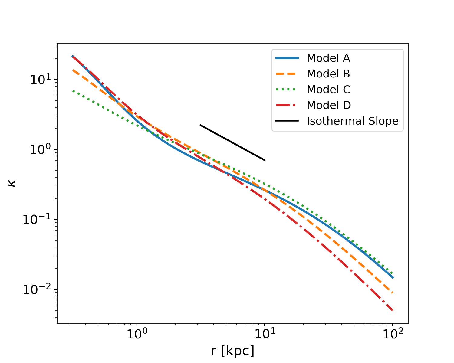 Figure 1
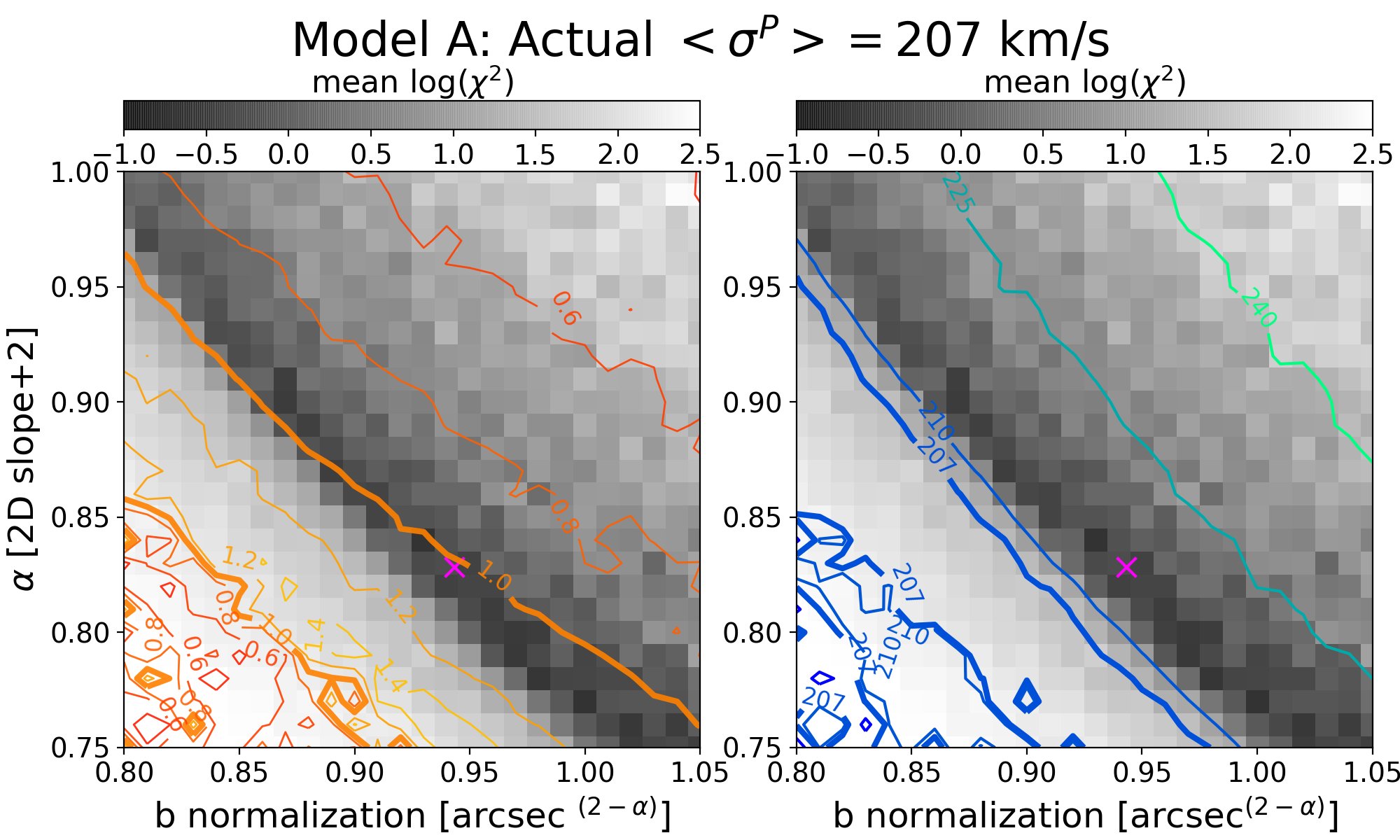 Figure 2
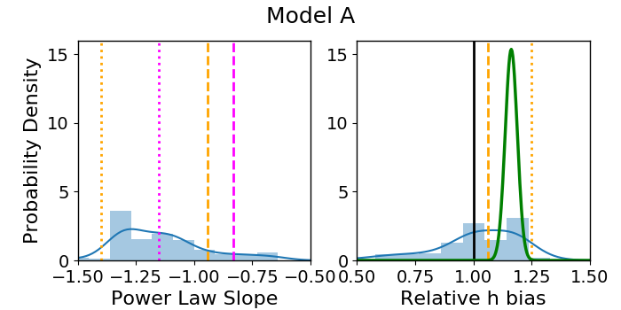 Figure 3
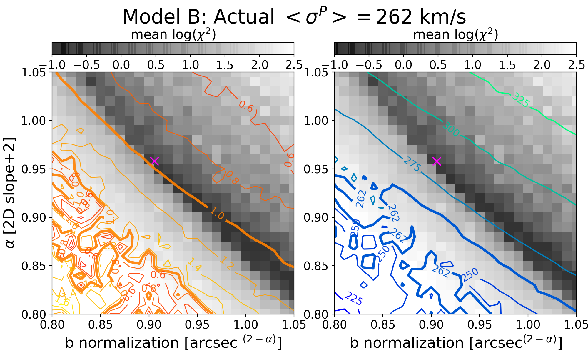 Figure 4
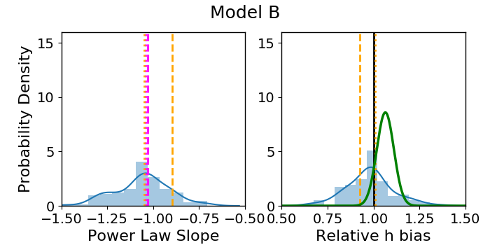 Figure 5
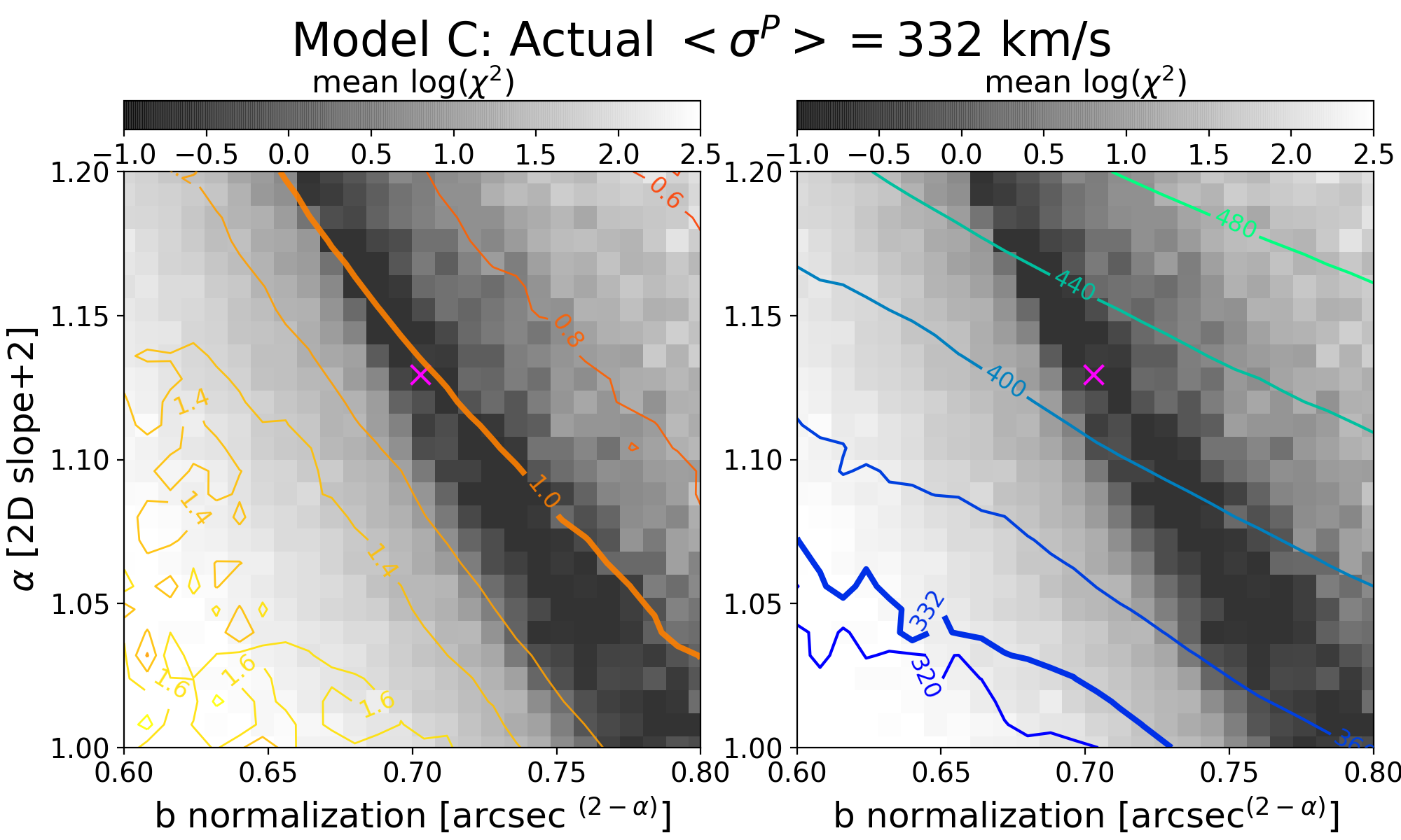 Figure 6
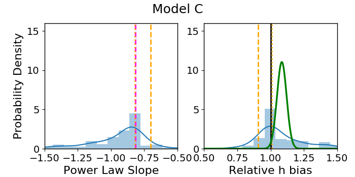 Figure 7
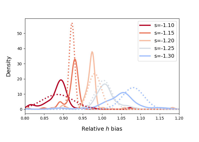 Figure 8
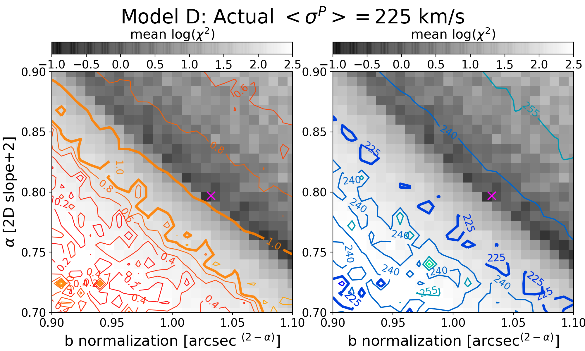 Figure 9
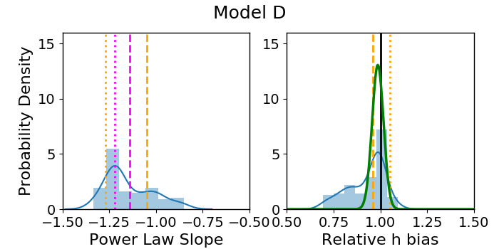 Figure 10
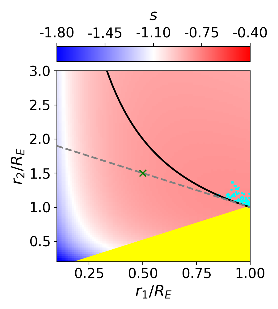 Figure 11
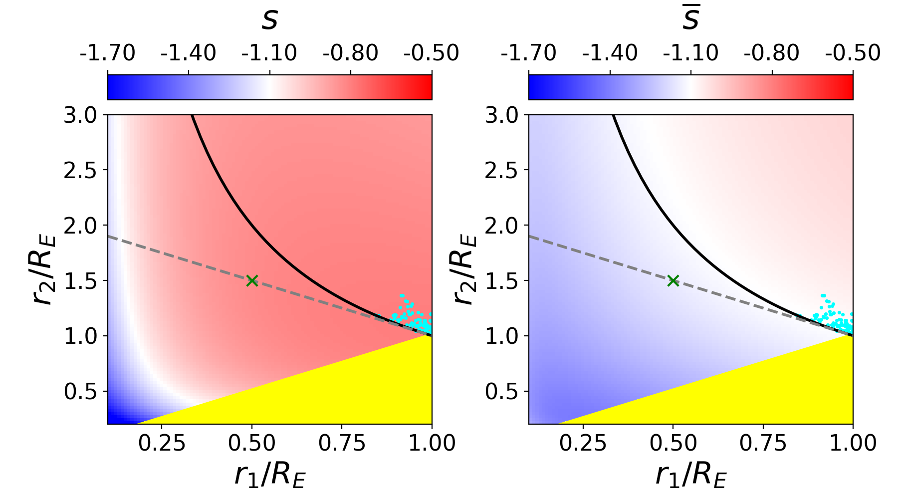 Figure 12
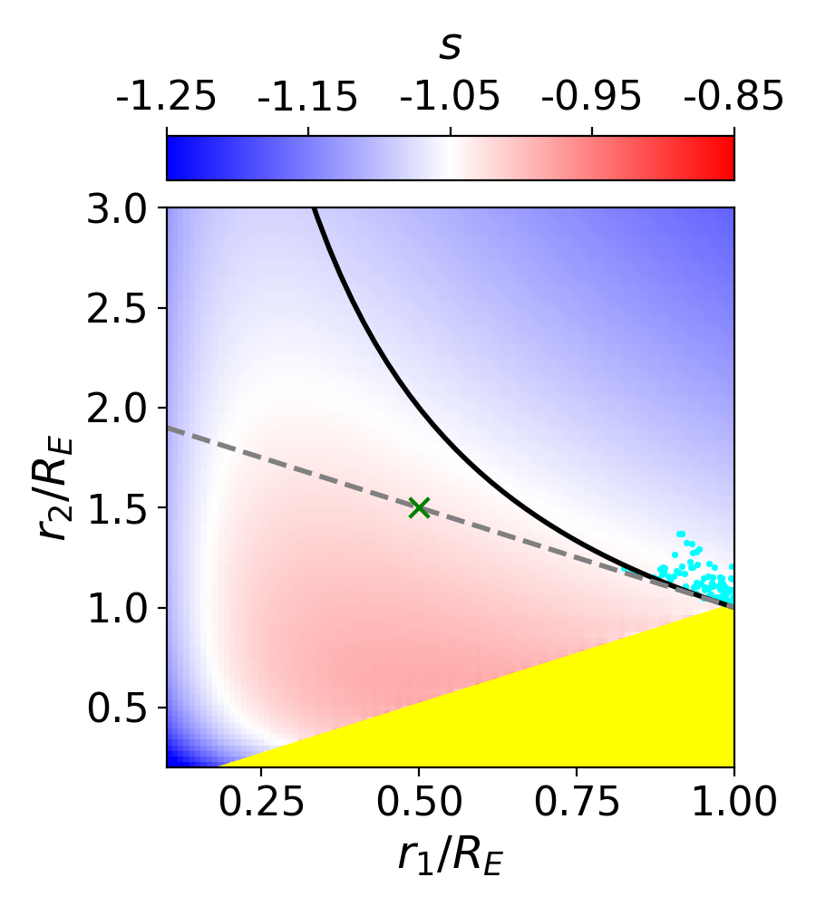 Figure 13
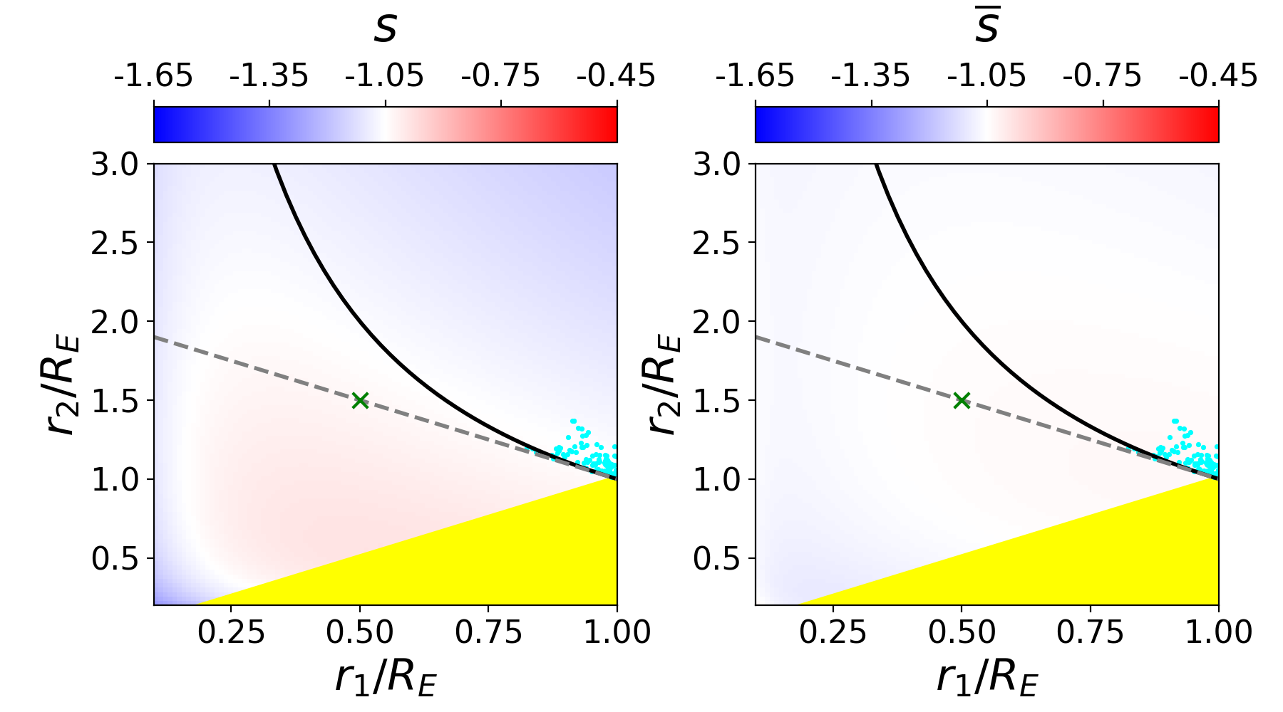 Figure 14
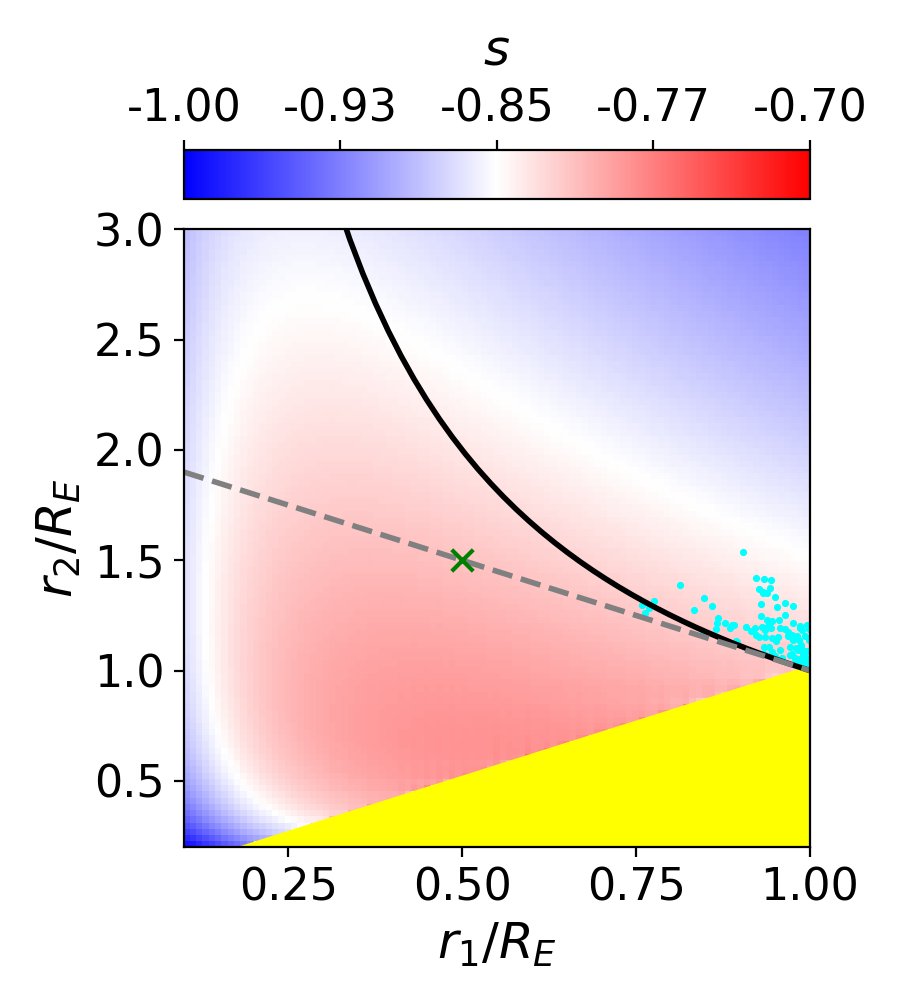 Figure 15
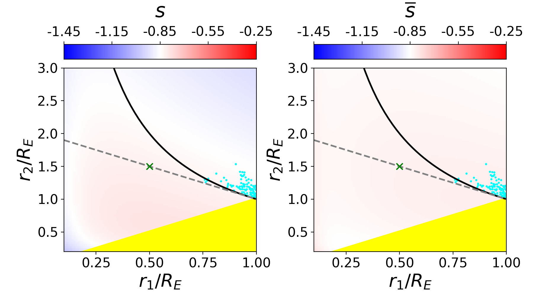 Figure 16
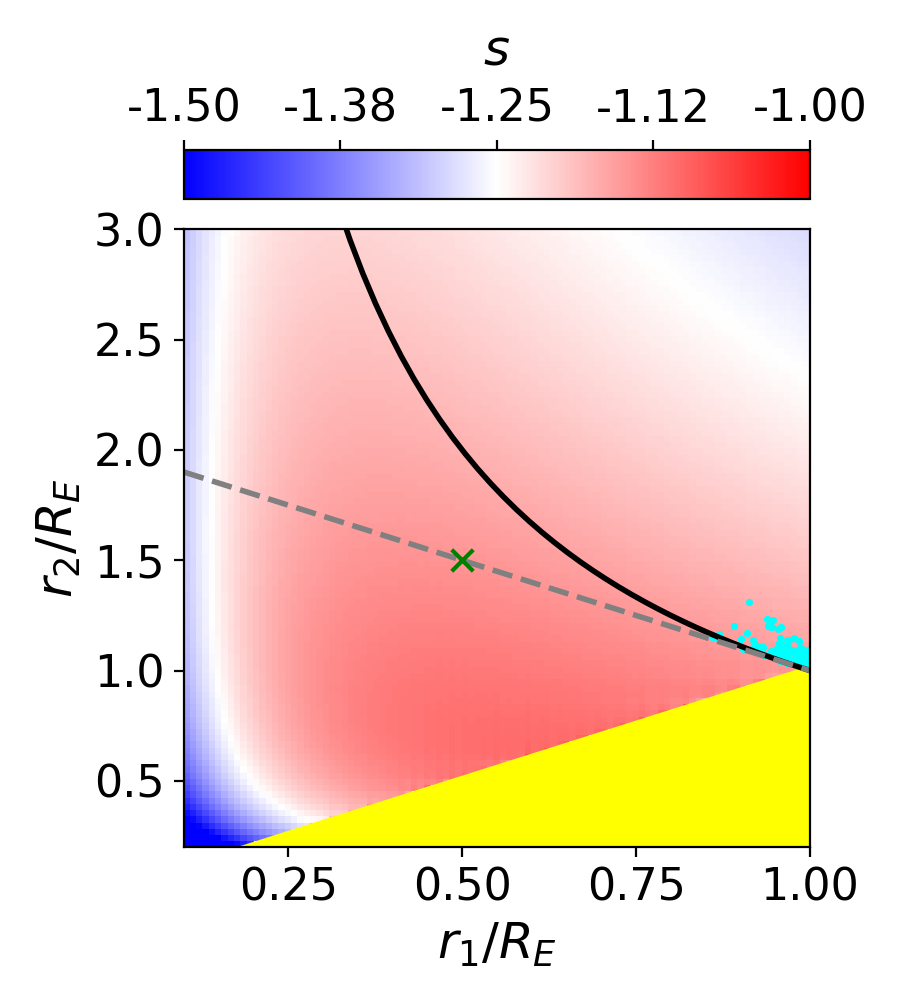 Figure 17
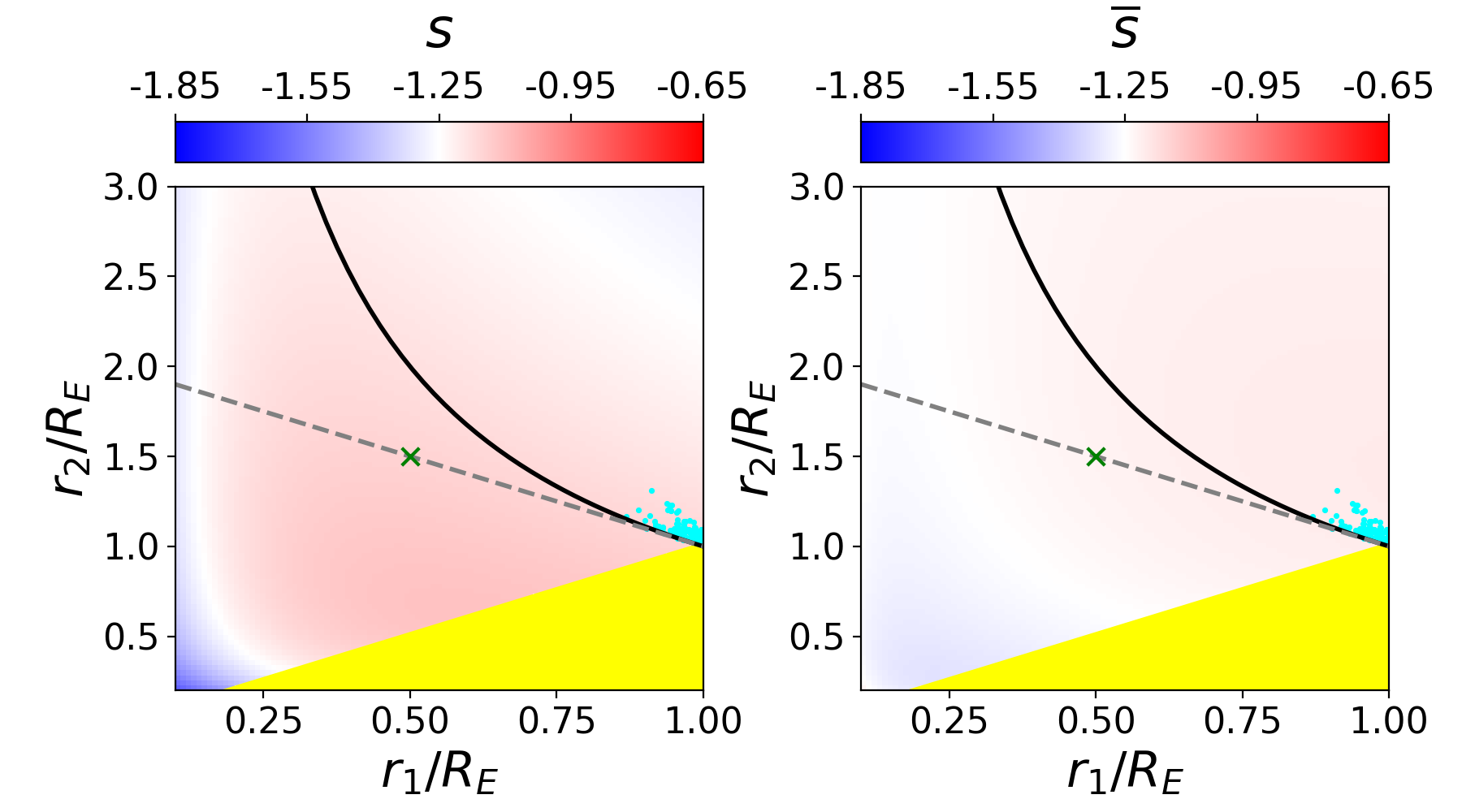 Figure 18
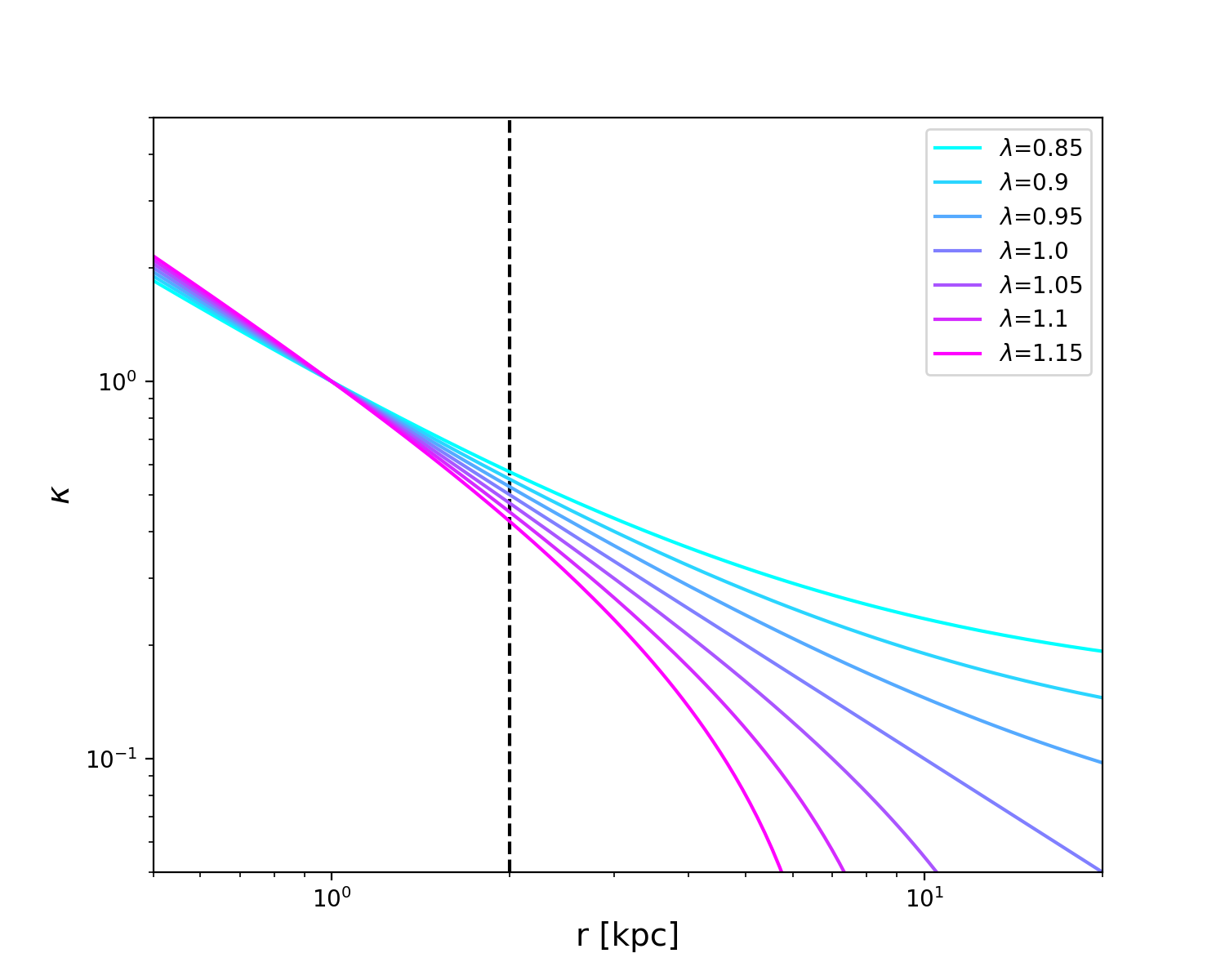 Figure 19
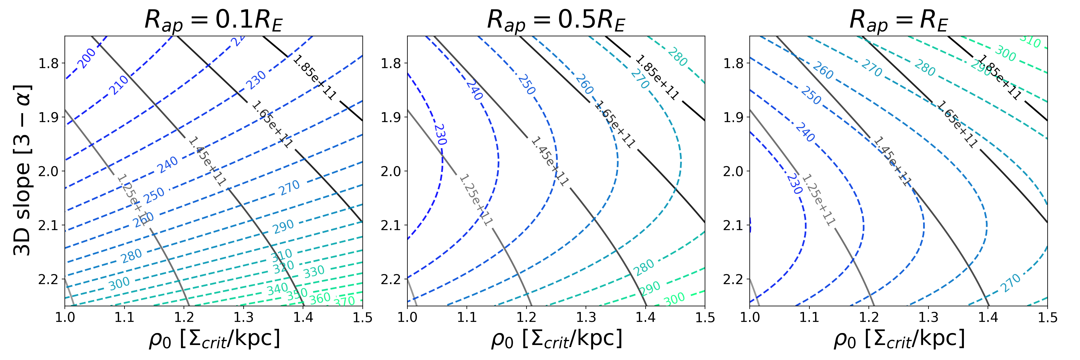 Figure 20
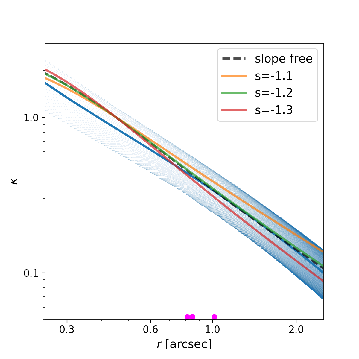 Figure 21
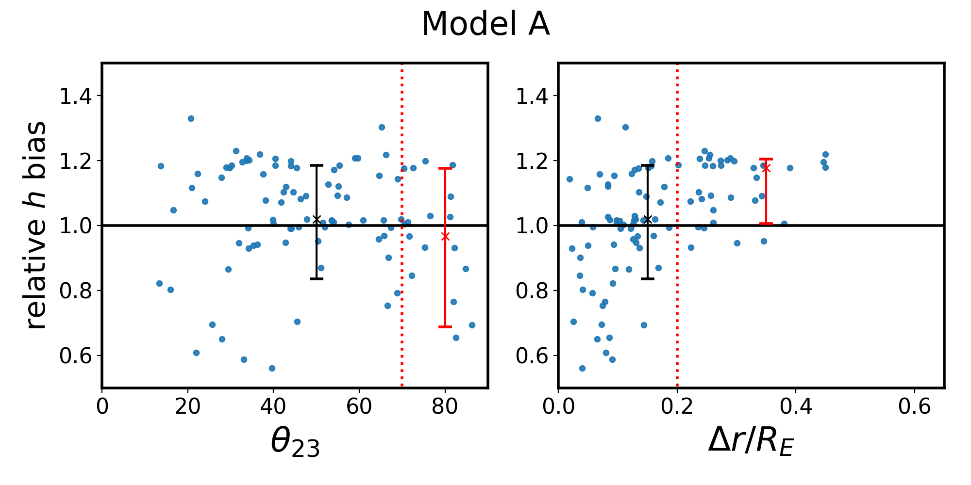 Figure 22
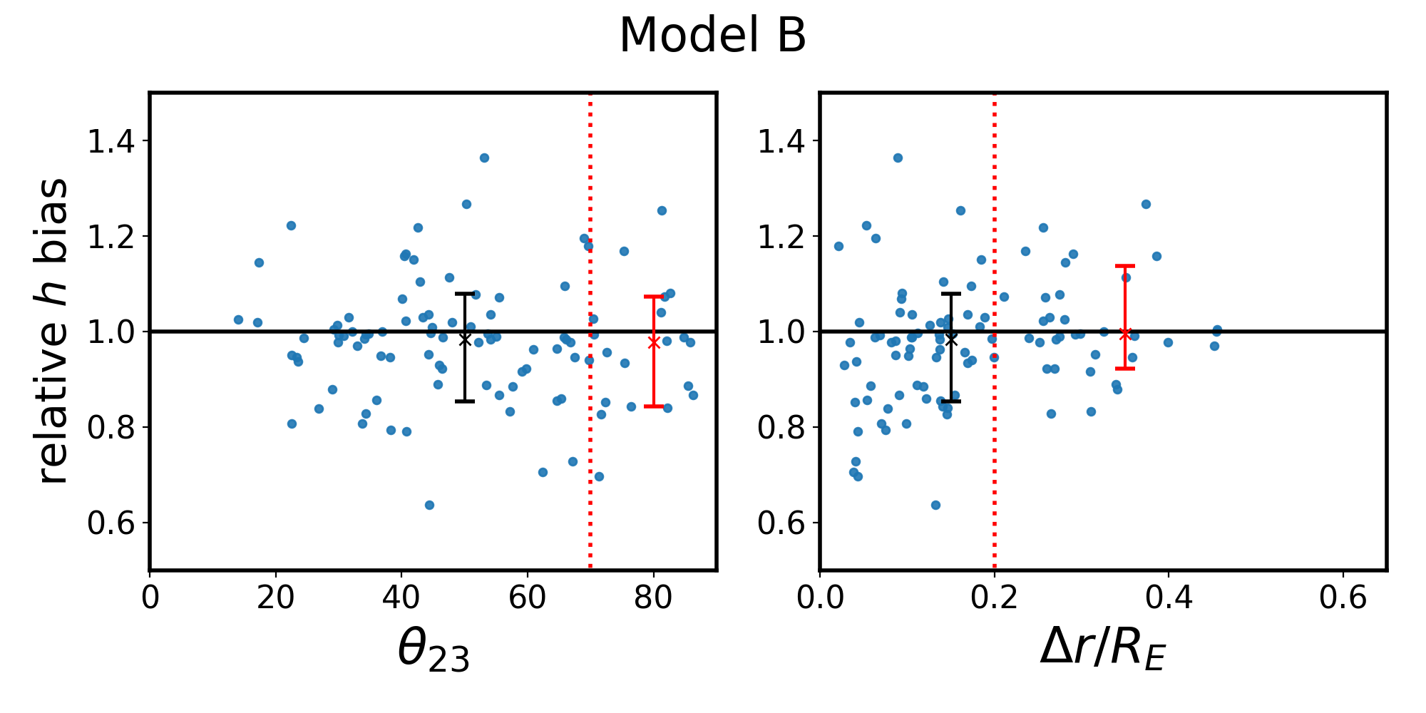 Figure 23
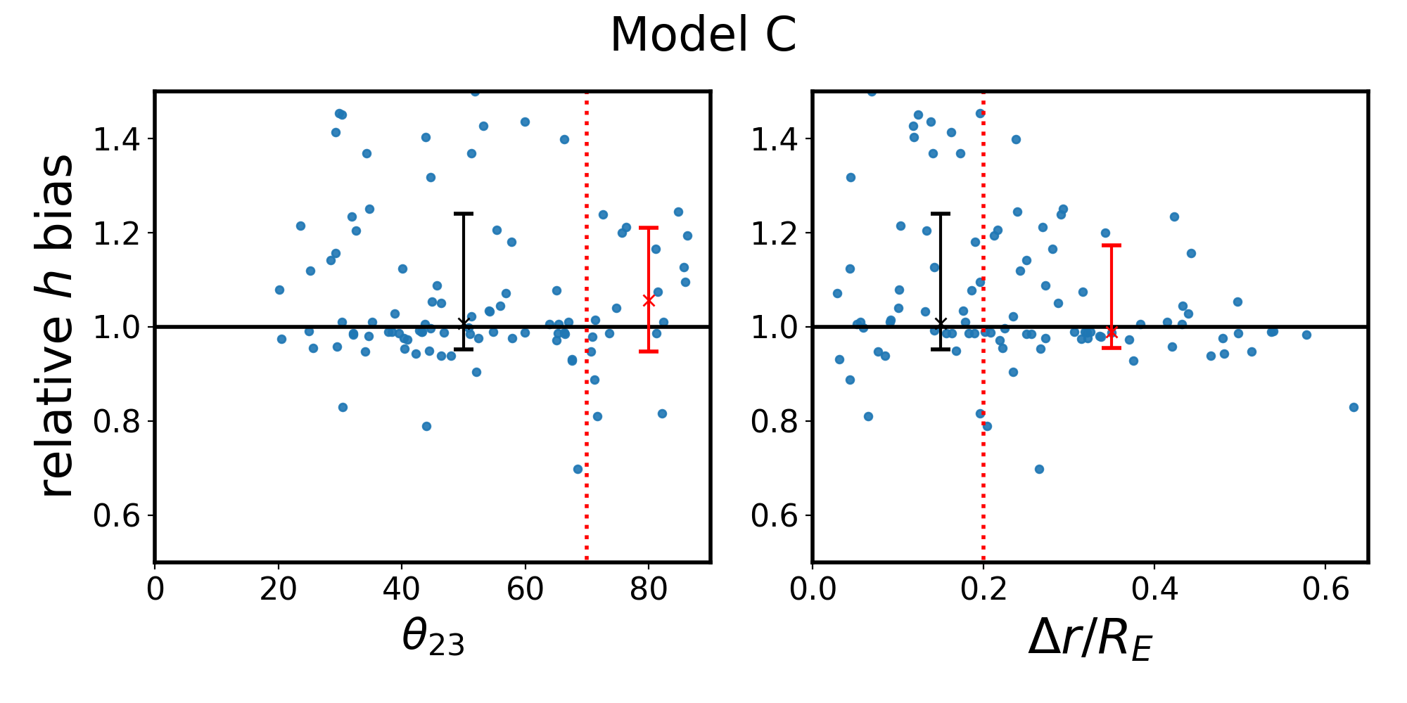 Figure 24
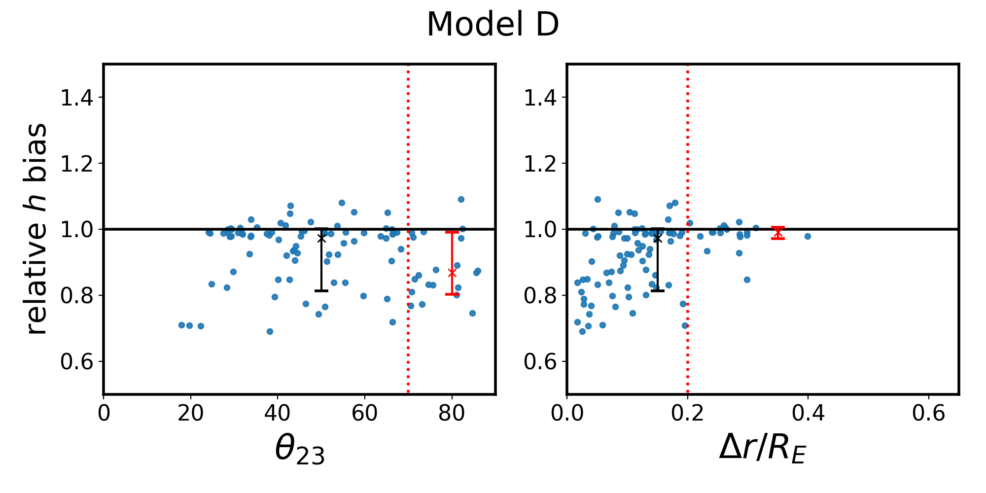 Figure 25
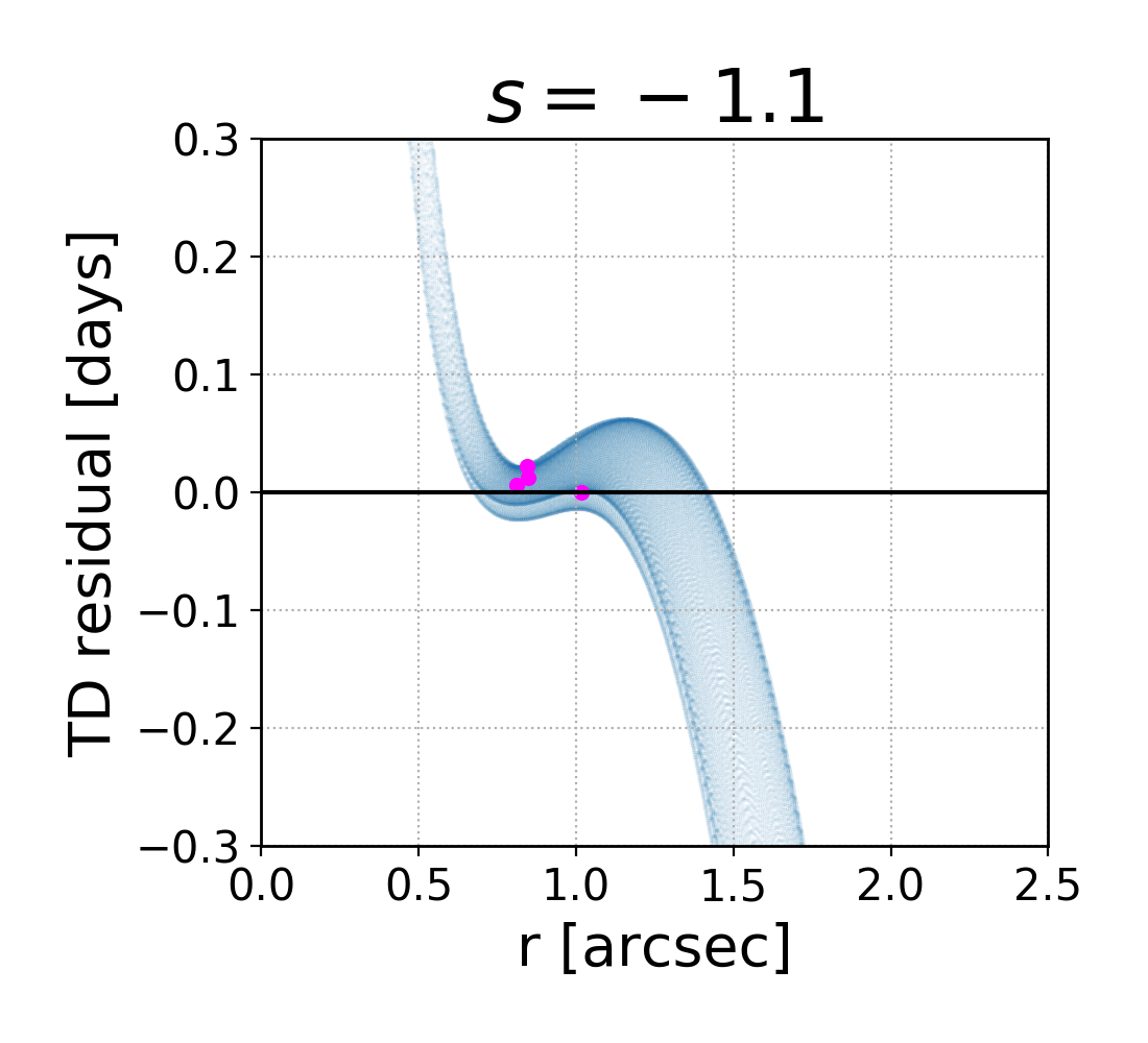 Figure 26
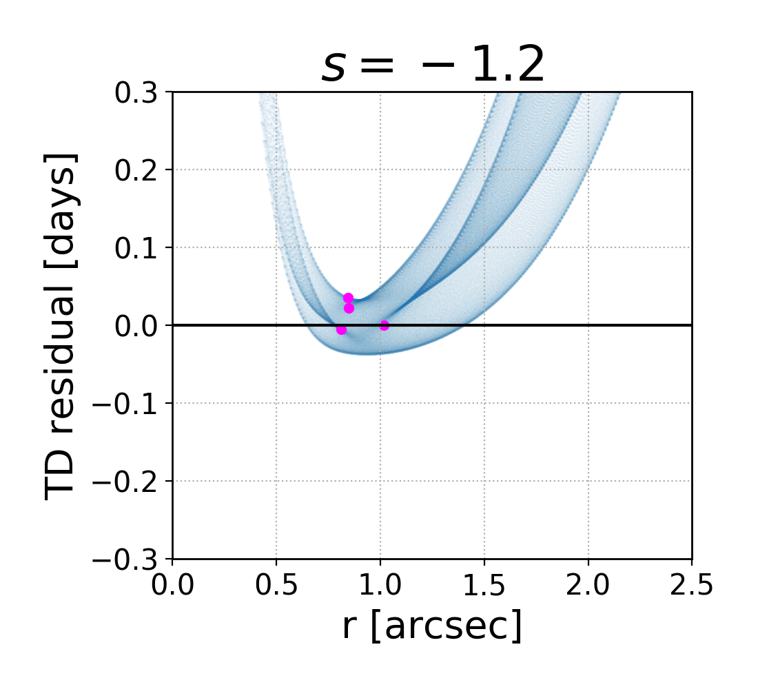 Figure 27
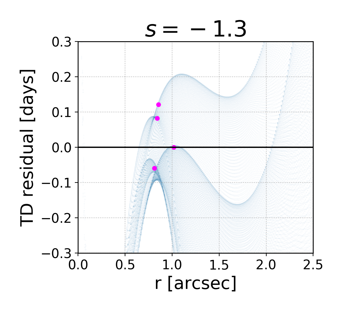 Figure 28
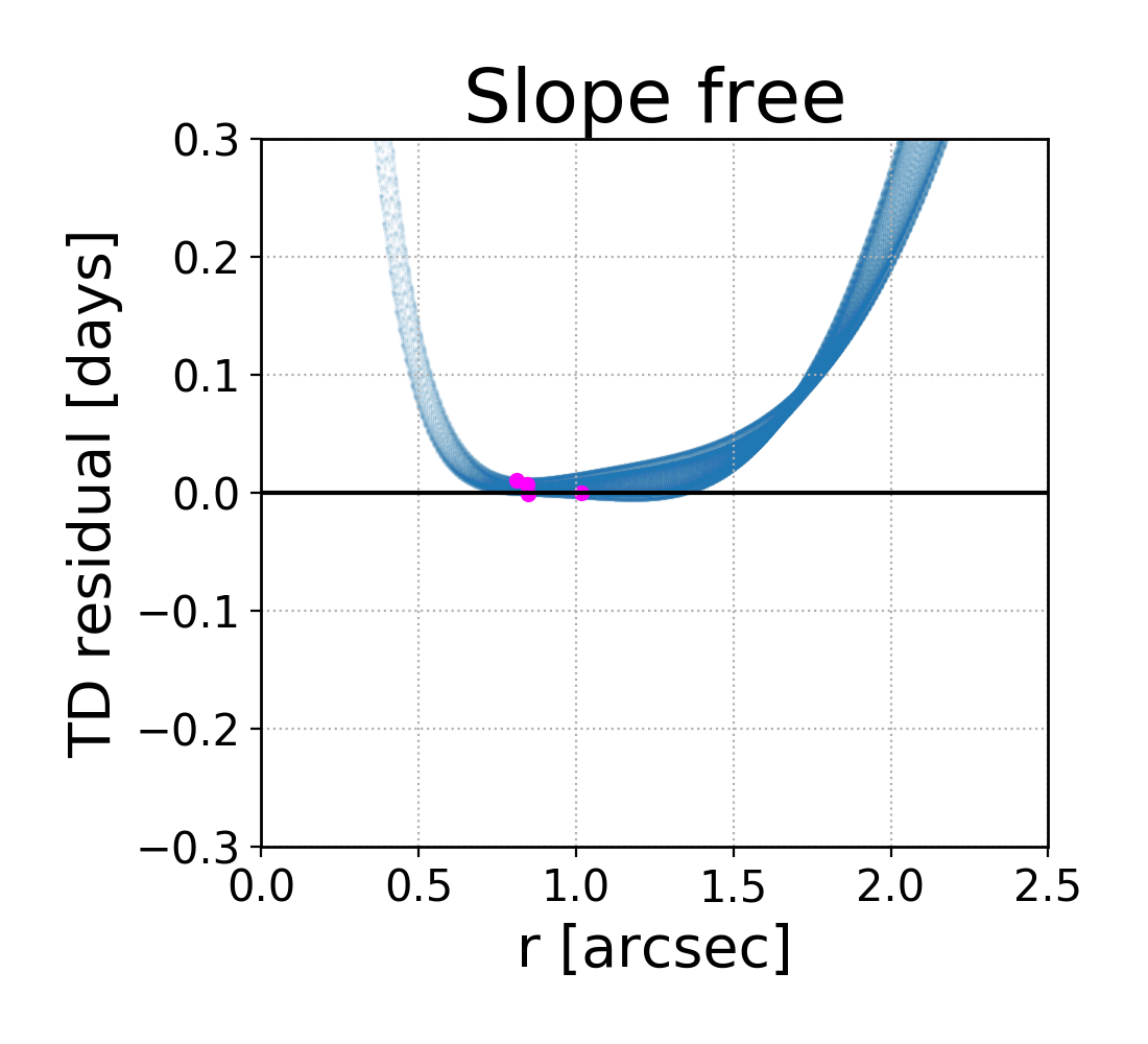 Figure 29
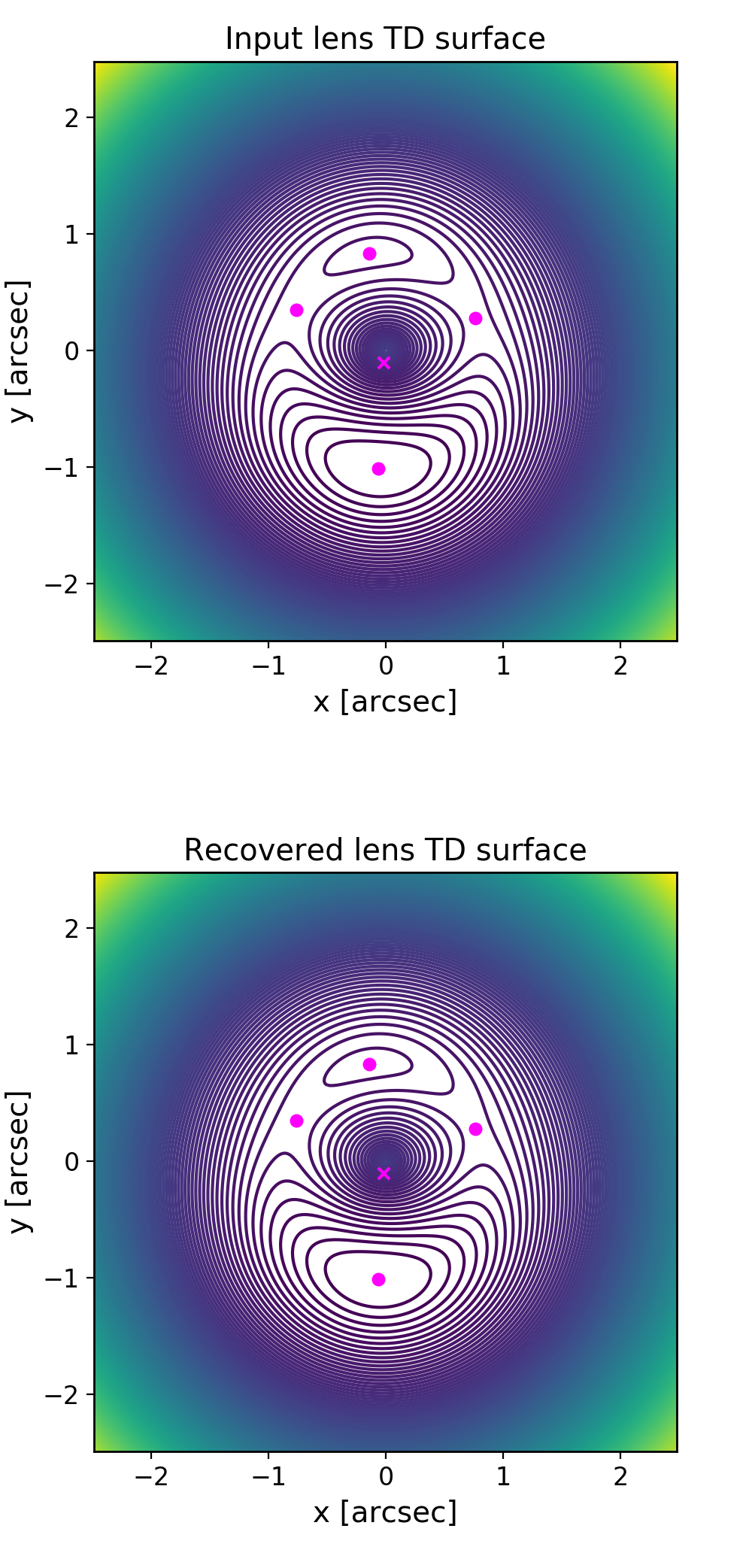 Figure 30
| Profile construction parameters | Resulting lens physical attributes | MST values | ||||||||||||
| Model | ||||||||||||||
| A | 0.30 | 30.0 | 30.0 | 0.12 | 5.1 | 1.7 | 0.81 | 271 | 9.0 | 207 | -0.830 | 1.06 | -0.94 | |
| B | 0.60 | 10.07 | 13.33 | 0.206 | 5.7 | 2.1 | 0.67 | 234 | 17.6 | 262 | -1.03 | 0.925 | -0.895 | |
| C | 0.816 | 3.76 | 22.25 | 0.157 | 4.9 | 1.6 | 0.68 | 291 | 13.1 | 332 | -0.815 | 0.904 | -0.702 | |
| D | 0.40 | 22.53 | 10.0 | 0.225 | 5.5 | 2.0 | 0.70 | 195 | 19.5 | 225 | -1.14 | 0.960 | -1.05 | |
| Parameter recovery: density slope free to vary | ||||||
| Model | MLE | Mean | ||||
| A | 1.06 | 1.25 | 0.011 | 1.00 | 0.99 | |
| B | 0.925 | 1.01 | 0.007 | 0.99 | 0.99 | |
| C | 0.904 | 1.01 | 0.008 | 1.00 | 1.00 | |
| D | 0.960 | 1.05 | 0.005 | 1.00 | 0.97 | |
| Model A | |||
|---|---|---|---|
| Slope | MLE | ||
| -0.85 | 0.97 | 0.67 | |
| -0.90 | 0.98 | 0.70 | |
| -0.95 | 0.98 | 0.71 | |
| -1.00 | 0.98 | 0.72 | |
| -1.05 | 0.97 | 0.58 | |
| -1.10 | 0.99 | 0.64 | |
| -1.15 | 0.99 | 0.60 | |
| Model B | |||
| Slope | MLE | ||
| -1.00 | 0.99 | 0.60 | |
| -1.05 | 0.975 0.014 | 0.97 | 0.64 |
| -1.10 | 0.99 | 0.55 | |
| -1.15 | 0.99 | 0.69 | |
| Model C | |||
| Slope | MLE | ||
| -0.80 | 0.98 | 0.70 | |
| -0.85 | 0.98 | 0.64 | |
| -0.90 | 0.97 | 0.65 | |
| -0.95 | 0.99 | 0.69 | |
| Model D | |||
| Slope | MLE | ||
| -1.10 | 0.99 | 0.69 | |
| -1.15 | 0.99 | 0.68 | |
| -1.20 | 0.97 | 0.62 | |
| -1.25 | 0.97 | 0.55 | |
| -1.30 | 0.99 | 0.67 | |
Peer Reviews
No public reviews on file for this paper yet. If you reviewed it on a platform where reviews are public (OpenReview, ICLR, NeurIPS, ICML), you can paste yours below so the community can read it here.
Videos
No videos yet. Explain this paper in a talk, walkthrough, or lecture? Add one.
Galaxy-lens determination of : constraining density slope in the context of the mass sheet degeneracy
M. Gomer,11footnotetext: Corresponding author.
L. L. R. Williams
Abstract
Gravitational lensing offers a competitive method to measure with the goal of 1% precision. A major obstacle comes in the form of lensing degeneracies, such as the mass sheet degeneracy (MSD), which make it possible for a family of density profiles to reproduce the same lensing observables but return different values of . The modeling process artificially selects one choice from this family, potentially biasing . The effect is more pronounced when the profile of a given lens is not perfectly described by the lens model, which will always be the case to some extent. To explore this, we quantify the bias and spread in by creating quads from two-component mass models and fitting them with a power-law ellipse+shear model. We find that the bias does not correspond to the estimate one would calculate by transforming the profile into a power law near the image radius. We also emulate the effect of including stellar kinematics by performing fits where the slope is constrained to the true value. Informing the fit using the true value near the image radius can introduce substantial bias (0-23% depending on the model). We confirm using Jeans arguments that kinematic constraints can result in a biased value of , though the degree of bias depends on the region kinematic modeling probes in specific lenses. We conclude that lensing degeneracies manifest through commonplace modeling approaches in a more complicated way than is assumed in the literature. If stellar kinematics incorrectly break the MSD, their inclusion may introduce more bias than their omission.
1 Introduction
Robust determination of the Hubble constant is one of the most sought-after goals in cosmology. Over the years, increasingly precise measurements of temperature anisotropies in the cosmic microwave background (CMB) have recovered values of with smaller and smaller uncertainties. At present, the most precise CMB constraints come from the Planck mission, which found km s*-1Mpc-1* (0.7% uncertainty), assuming CDM cosmology [1]. Baryon Acoustic Oscillation (BAO) results from the Dark Energy Survey are broadly consistent with CMB results [2].
Meanwhile, standard candle observations using Type Ia supernovae and Cepheid variables provide a direct distance measurement to faraway galaxies, allowing to be measured directly rather than recovered from a model with many parameters [3]. The tradeoff is that this method is dependent on the calibration of these standard candles, where any uncertainties in local measurements propogate to farther measurements. This method has been able to compete with the precision of CMB observations and, through improvements in the calibration, has presently determined value of km s*-1Mpc-1* (1.91% uncertainty) [4].
Tension exists between these two methods at the level. The cause of this tension is unknown at present. These two methods compare the directly-measured local value of to the most distant possible determination at the time of recombination, meaning they probe the expansion of the universe from one end to another. It might turn out that the prevailing model is more complicated than CDM, hinting at new physics beyond the standard model or general relativity, perhaps through time-dependent dark energy or some other mechanism [3]. On the other hand, it might turn out that the uncertainties of these two methods are missing some source of systematic error, and are thus underestimated. If the Milky Way resides within a local void, the measured value of will be systematically biased with respect to the true value, although at present it does not seem that this effect would be sufficient to resolve the tension [5, 6]. Perhaps the answer lies in the standard candle calibration– Freedman et al. [7] recently found that replacing the Cepheid variable calibration with the Tip of the Red Giant Branch (TRGB) distance indicator results in a lower value of stat sys km s*-1Mpc-1*, only away from the CMB result. It might turn out to be random chance that the methods disagree and as more data is collected they may converge to the same value. To diagnose the existence of the tension between these methods, an additional independent method would be exceedingly useful.
Strong gravitational lensing offers this independent method. If a variable source is multiply imaged, the difference in arrival time between the images offers a measurement of the time delay distance, [8]. If one has an accurate model of the lensing potential for the mass distribution of the lens, it is straightforward to measure from such information [9, 10, 11]. The challenge is to precisely determine the time delays and lensing potential.
At the cluster scale, multiple sources provide additional constraints to the potential and allow one to mitigate the effects of the mass-sheet degeneracy (see Section 1.1). Using parametric models which implicitly assume that the galaxies within the cluster have similar mass profiles to isolated galaxies in equilibrium, constraints on have been estimated at the 6% level, with 40% uncertainty on [12]. When this assumption is relaxed through the use of free-form modeling, the lensing potential is considerably more complicated, producing larger uncertainties in [13]. Because of this, the strongest constraints will likely come from the scale of individual galaxies, which will be the focus of this paper.
Improvements in the method over time have enabled constraints on to be placed at the 7% level using a single system [10, 14]. Further improvements can be gained by combining constraints using multiple systems to average over variations between individual lenses. The tightest constraints from this method come from the state-of-the-art H0LiCOW ( Lenses in COSMOGRAIL’s Wellspring) program [11]. H0LiCOW gets time delays from the COSMOGRAIL (COSmological MOnitoring of GRAvItational Lenses) program [15, 16], which has been monitoring light curves of multiply imaged systems for 15 years to date, measuring time delays within 1-3% uncertainty [17, 18]. H0LiCOW models lenses using image positions, fluxes, and time delays, as well as stellar kinematics of the lens galaxy [19]. The analysis incorporates a variety of effects, such as inclusion of nearby group members [20] and an estimation of line-of-sight external convergence [21]. Most recently, a blind combined analysis of six systems yielded a measurement of km s*-1Mpc-1* (2.4% uncertainty) [22].
In order to provide insight into the nature of the tension, the uncertainty in the method must be competitive with the existing methods. The ambitious goal of the community is to reduce the uncertainties of the time delay method to 1% [11]. Bonvin et al. [23] outline four actions which must be taken in order to reach such high precision: 1. Enlarge the sample, 2. Improve the lens model accuracy, 3. Improve the mass calibration through spatially resolved kinematics, and 4. Increase the efficiency of time delay measurement techniques. While the other actions are certainly important, the focus of this paper will be on the second and third: improving the lens model accuracy and studying the role of kinematic information. As Bonvin et al. [23] put it, “as the number of systems being analysed grows, random uncertainties in the cosmological parameters will fall, and residual systematic uncertainties related to degeneracies inherent to gravitational lensing will need to be investigated in more detail." Put another way, the statistical scatter due to a small sample size will decrease with time, but any biases inherent to lens modeling will not go away, potentially offsetting the recovered value from the true value. It is crucial that all biases intrinsic to the modeling process are carefully accounted for.
1.1 Effect of lensing degeneracies
The source of the problem comes from lensing degeneracies, where the same observables can be recovered with multiple different lens models. There exist many types of degeneraries, the most famous of which is the exact mass sheet degeneracy (MSD) [24], where image positions and relative fluxes are left unchanged by a rescaling of the profile normalization and the corresponding introduction of a uniform convergence.
[TABLE]
Meanwhile, does affect the product of and the time delay: , meaning that the recovered value of will be biased by a factor of . For any lens model, the MSD allows for flexibility in the profile shape, since a range of profiles with varying would all reproduce the same observables. In principle, any of those profiles are equally supported by the data, but in practice, only one is chosen by the modeling process [25]. The effect of the MSD on a power-law shape is illustrated in Figure 1 for several values of . During modeling, the lens profile is assumed to follow a simple analytical shape, like a power law or a NFW profile. This forces to take on the particular value that makes the profile fit that shape in the region where images are located. In this way, a simplifying assumption could impose a value of (and therefore ) which is not necessarily the same as the true mass distribution, as it has been artificially selected by the model choice.
It is worth emphasizing that this systematic effect is caused by lensing degeneracies inherent to all lens modeling and is not specific to any particular profile. Though this paper will be specifically exploring the effects with respect to a power-law model, any other profile would also be biased toward the particular value of which causes the mass distribution to most closely match the assumed profile. Even sophisticated methods which use a Bayesian framework to determine the most likely of multiple different models (such as Autolens, Nightingale et al. [26]) will be subject to systematic effects of degeneracies, although the nature of the systematic effects will likely be correspondingly more intricate. The exploration of these effects must start with simpler lens models.
The combined effect of the MSD and simplifying assumptions about the density profile shape has recently been analyzed by Xu et al. [27]. The authors extracted galaxies from the Illustris simulation along different lines of sight and looked at their lens profiles. They calculated the necessary to transform each profile into a straight power-law shape (with slope ) near the image radius and assumed that this would be the value of the multiplicative bias on a lens modeler would recover when fitting the system with a power-law profile. They found that the mean deviation of from unity can be as large as 20-50% with a scatter of 10-30% (rms). Even limiting their sample to the galaxies which recover a slope near isothermal resulted in a systematic deviation with a scatter of 10%, implying that the power-law assumption introduces significant bias in the recovery of . More recently, Tagore et al. [28] performed a similar analysis using galaxies from the EAGLE simulation, with similar results. Tagore et al. [28] continued their analysis by supplementing the lens systems with aperture velocity dispersion information. After using a joint model analysis and omitting lenses with poor , they found that double image lenses were still biased at the 7% level. Quad lenses were less biased, with the cross quads specifically being the least biased at the 1.5% level (Table 7 and Figure 11 of Tagore et al. [28]). It may yet turn out that the improvement and inclusion of kinematic information, combined with clever selection criteria, can help to mitigate the effects of the MSD.
Despite this finding, caution is advisable. Both Xu et al. [27] and Tagore et al. [28] extract lens profiles from state-of-the-art simulations, which may not have the resolution to describe the inner radii in sufficient detail. In particular, both studies selected galaxies with , where is the Einstein radius and is the gravitational softening length of the simulation, and calculated slope and by using measurements at , i.e. as small as . These findings are dependent on the simulations being well-resolved at just one softening length. This concern is exacerbated by the recent work of van den Bosch and Ogiya [29]. By analyzing a simplified case of a dark matter subhalo orbiting a static potential, they found that tidal distruption of subhalos within simulations is predominantly a numerical phenomenon rather than a physical process, implying even cutting-edge simulations may not be fully converged.
Even relatively small discrepancies between the lens model and the actual profile are cause for concern because first-order perturbations to the profile can produce zeroth-order changes in time delays and therefore [30]. Additional cause for alarm has recently been shown by Kochanek [31] and Blum et al. [32], who demonstrated, using different means, that lens models with oversimplified or wrong assumptions can lead to high precision, but inaccurate determinations of . Kochanek [31] concluded that cannot be more than accurate, despite claims of higher precision.
The goal of this paper is to quantify the bias and spread in the recovery of , both with and without the inclusion of stellar kinematic constraints. Rather than drawing lens profiles from simulations, we will create lenses from two-component analytical profiles, constructed to represent both baryons and dark matter. Because of this, the true profile shape is well-known beforehand.
This investigation is a controlled study, with the intention being to test the effects of model assumptions on relatively simple profiles rather than attempting to perfectly mimic real galaxies. Real galaxy profiles do differ from a power law (or any assumed model), but the deviation from a particular model is dependent on the galaxy. While a particular model profile might provide a good description for a population of galaxies, individual galaxies vary, and will deviate from the model by varying amounts. Simulated halos have significant variance in their shape parameters [33], and still lack self-similarity even when baryons are included [34]. Galaxy profiles may be well-approximated by power laws at the 10% level [31], which has been adequate for galaxy-formation science, but is a large amount of deviation when compared to the 1% goal. Our synthetic lenses (Figure 2) are consistent with real galaxies, but their deviation from a power law is in a known and controlled way, rather than the random, unpredictable deviation of real galaxies. This serves as a starting point to test the effects of the power-law assumption.
From these lenses, quads will be created. The image positions and time delays will then be fit using a simple power-law ellipse+shear model, a common model for real systems. We will then compare the resulting slope and with the expected value of and predicted by Xu et al. [27]. Such agreement, which the authors assumed, would mean that it is possible to calculate the bias given the profile shape from simulations, while disagreement would mean that the MSD manifests in a more complicated way which is less straightforward to calculate.
In practice, stellar kinematic information can be used to provide an absolute measure of mass, breaking the mass-sheet degeneracy [14, 35]. This extra information is hypothesized to reduce the bias and the spread of . We will explore this hypothesis in two ways. In Section 5.1, we test the effects of constraining the slope in the parameter recovery. This emulates the additional constraint of kinematics through the inclusion of external information about the mass profile. In Section 5.2, we calculate the integrated velocity dispersion using a spherical Jeans approximation. We compare the velocity dispersion for the actual profile with what one would find if the profile were the power-law recovered from the lensing information. A comparison of these values allows us to diagnose whether or not kinematic information can correctly break the MSD when the mass model is slightly oversimplified.
Throughout this paper we will use km s. Lenses are constructed with .
2 Preliminary Tests
We will be fitting quads using the lensmodel application [36]. The application inputs observational constraints combined with a choice of parametric model, then fits the system using the calculated by comparing the modeled images to the observed constraints. This application has been used to model strong lens systems in a variety of studies (see Lefor et al. [37] and references therein). Though lensmodel is capable of using image fluxes and extended images, we will simply evaluate using image positions and time delays as our observable quantities, assuming optimistic observational uncertainties of 0.003 arcseconds in spatial resolution and 0.1 days in time delay measurements. This spatial resolution is too precise for optical telescopes, but is feasible using VLBI measurements in the radio, which is currently being done for lenses in the strong lensing at high angular resolution program (SHARP, Spingola et al. [38]). We use this uncertainty in the spirit of making the strongest possible constraints on a lens model. The first step we must take is to confirm that we are able to accurately recover lens parameters from our mock quad images. We conducted several initial experiments to confirm this.
We wish to adopt a commonly-used analytical model with simplifying assumptions about the mass distribution of the lens. Specifically we choose to fit the lens with a ellipse+shear power-law model, which has 7 parameters: mass normalization, ellipticity, ellipse position angle, shear, shear angle, core radius, and slope. Since there are 9 observations (6 relative image coordinates and 3 relative time delays) there are degrees of freedom.
Specific to lensmodel, we experimented with the alpha and alphapot models, which are a power-law mass distribution and lensing potential, respectively. Our preliminary tests were on several basic lenses, some matching the power-law forms of the fitting models and some using other profile shapes (namely the two-component Einasto profiles of Gomer and Williams [39]). Limited to a cursory search using only a few quads, in some cases the lens parameters were successfully recovered. For other quads we were less successful, leading us to several main findings:
For some quads, fitting for two parameters in a different order resulted in a better or worse fit. This custom-tailored parameter search is only possible for a small number of quads modeled on an individual basis. 2. 2.
Despite the optimization routine of lensmodel, the recovered slope frequently gets stuck at a local minimum near the initial slope guess. We also occasionally found that restarts of the optimization routine would drastically depart from the nearby minimum and return bad fits. 3. 3.
Lenses created from power-law mass distributions (as opposed to lensing potential) had parameter recoveries which were worsened by pixelation and the finite window of lens construction. 4. 4.
Lenses created from Einasto mass distributions frequently had poor parameter recovery when assumed to be a power law. This is likely due to a combination of the numerical effect above and the MSD power-law assumption biasing the recovery of parameters.
We will have too many quads to model each in a unique way, such as customizing the order in which parameters are fit. Interestingly, this problem is becoming relevant for real lens systems as well, as the number of known systems continues to grow. Since human supervision is not feasible at this scale, automation must be the way forward. For real lens systems, automated fitting procedures such as Autolens [26] are already being developed. Our modeling is significantly less sophisticated, but will still require an automated algorithm which tries several different runs in lensmodel to find good fits for each quad in a uniformly controlled way.
Our fitting procedure is devised specifically to avoid the pitfalls of (1)–(4). Here we define our method explicitly. The procedure is nearly identical to the example in Keeton [36], with one extra step. The first run fits the quads with only the mass normalization free to vary, while searching a grid over all values for the position angle and shear angle. All other parameters are held at fiducial values for this first run. The robustness of this process against changes to these fiducial values is detailed in Appendix A. Next, a run is executed which uses the best fit result from the previous run as an initialization. This second run allows mass normalization, position angle, and shear angle to vary while searching a grid over values of ellipticity and shear. The third run initializes using the best-fit result of the second run and allows all 7 parameters to vary. This third run implements the “optimize" routine of lensmodel, which uses the amoeba algorithm available in Press et al. [40], restarting several times to ensure that the result robustly returns to the same minimum. The last step is an additional step we have added to make sure the slope recovery does not get stuck at a local minimum. This step restarts the process at the first run, with a different initial value for the slope. Once the process is completed over the desired range of slope initializations, only the single result with the lowest is kept. This result is the best fit for this model for a single quad, as the procedure systematically searches over the relevant parameters with a variety of initializations and restarts. To circumvent the problem arising from using mass distributions, from now on we will only construct lenses created via analytical lensing potentials (power law or NFW), fit using a power-law potential via alphapot. This requirement means we can no longer use the Einasto form of the lenses constructed by Gomer and Williams [39].
3 Lens Construction
Now that the numerical effects of the process have been limited to the best of our ability, we are ready to create our set of lenses. The lenses are constructed through the combination of two components: a baryon power-law component (alphapot) and a dark matter NFW component, which is analytically expressible as a lensing potential [41, 42].
[TABLE]
where
[TABLE]
and
[TABLE]
with
[TABLE]
Ellipticity is introduced through , where is the axis ratio of the potential. For the NFW component, such that ellipticity is introduced in a consistent way, where is the scale radius of the NFW profile. In total, six parameters are required to make a lens: , , , , , and . The core softening radius, is set to 0.3 kpc. Note that the 2D slope of the power-law mass distribution will be equal to . Lenses are placed at a redshift of .
The cornerstone of the interpretation of Xu et al. [27] is that the value of calculated from the radial profile will be equivalent to the bias on . To test this, we experiment with a few different sets of values for the parameters which go into making our lenses (baryon normalization, , and slope, , as well as dark matter normalization, , and scale radius, ) to create a few different values of and see how is recovered in all cases. The choice of profile is somewhat difficult, since many options are physically reasonable. We settle on four different parameter choices of this class of profile, plotted in Figure 2 with their values summarized in Table 1. All of these four models are comparable to real galaxies. The Einstein radii, virial radii, and masses are consistent with the EAGLE simulation [28]. Like real halos, the profiles are nearly isothermal power laws at the Einstein radius (Fig. 2), and the velocity dispersions are consistent with actual lenses [10, 19]. We consider Model D to be the best analog to a real galaxy due to its slope being slightly steeper than isothermal which is in good agreement with real halos [43]. Meanwhile, Model A represents the most drastic departure from a power-law model, as evidenced by its visible curvature.
The process to calculate and is quite simple: choose a region near the Einstein radius over which the slope, is calculated. The magnitude of the mass sheet transformation (MST) necessary to transform the profile into a power law within that chosen region is , while the corresponding new slope after the MST is (Equations 4 and 10 of Xu et al. [27]).
It should be noted that the same argument can be applied with respect to deflection angle instead of convergence. Xu et al. [27] run the same analysis using the mean within a radius, referred to as , with slope . To assume a power law in would be similar to the assumption of a power law with respect to deflection angle. Applying the necessary MST to achieve such a power law would result in a bias and new slope . One advantage of this distinction is that deflection angle is a fundamental lensing property, unlike convergence, which is inferred. Therefore, we must also compare the recovered bias to the analytical prediction of the bias using .
One subtlety here is that the bounds over which the calculation is done are somewhat arbitrary– Xu et al. [27] and Tagore et al. [28] use and and these are the bounds used for the values calculated in Table 1, but other choices for the bounds are no less valid. Because the slope changes with radius, other choices for the bounds return different values of , and . This will be further explored shortly.
For a given model, 100 lenses are created, each producing 1 quad. Each lens is given an axis ratio between 0.85 and 0.99 in the potential, which roughly corresponds to between 0.5 and 0.99 in mass. This range is motivated because values more extreme than in potential results in mass distribution contours which become “peanut-shaped” rather than elliptical. The 100 quads are then fit by the automated process in Section 2, returning values for the 7 parameters, , and .
We intentionally choose to fit the lens systems with a model (power law) that does not have the same shape as the density profile (NFW + power law). In real systems, the true mass profile of an individual lens is not directly observable, but some model is assumed based on other studies of a population of galaxies. No individual galaxy will perfectly match the model profile, so this is always the case to some degree. Most studies assume that if the image positions are reproduced, then the lens model sufficiently matches the true mass distribution, but Schneider and Sluse [25] found that this effect can result in significant bias on . Using a method which explicitly separates the local data-based image constraints from the global model-based assumptions, Wagner [45] showed that image properties can be reproduced without reliance on global assumptions i.e. such that many different global mass distributions are viable. The use of a particular parametric model selects one of these mass distributions over the others, despite not being inherently preferred by the data. Instead, the selection comes from our assumptions about the shape of galaxy profiles in general. Since we can never have perfect knowledge of what the correct profile shape is for a particular galaxy, the effect of our ignorance must be included when seeking to evaluate our ability to fit lensing parameters.
[FIGURE:]
4 Results
We are primarily interested in the statistical results of an array of quad systems. Nonetheless, we have more deeply explored a particular quad from Model D to make certain that the image positions and time delays are properly recovered. We share these fittings in Appendix B. Confident that our procedure works, we are ready to discuss the results of the population.
4.1 Parameter recovery: density slope free to vary
The most straightforward way to represent the results is to plot a histogram of the best-fit values of slope and , shown in Figure 3 as the blue distribution for each of the four models. Nearly all () fits returned . The few cases with bad fits are omitted from the blue distributions, meaning all of the recovered parameters in the figure are within the uncertainties of observations. As an additional test of modeling success, we checked to see if the recovered ellipticities are strongly correlated with the true ellipticities, and find a Pearson coefficient after omitting the few cases with . Our lenses have zero input shear, and the recovered shear values are nearly zero. This tells us that not only do the image positions match, but the mass model parameters correspond quite well to their true values. These measures of fitting success are included in Table 2.
While useful, the blue histograms in Figure 3 do not fully capture the process of determining a single value of from many quads. As the number of systems increases, the shape of the blue distribution will stay roughly the same and will not narrow (see Appendix A), as it only returns a single value for each quad and does not combine them together in any way. Meanwhile, determinations of such as those presented by Wong et al. [22] and Tagore et al. [28] represent posterior distributions of from a single system, as well as aggregated together for a composite distribution from a number of systems.
To evaluate this, we use the varyh function in lensmodel to calculate the for a range of values near the best-fit value, marginalized over the other fitting parameters. 222 This is not strictly equivalent to the posterior distribution one would obtain from an MCMC sampling, but is meant to approximate the distribution. See Section 5.4. We then calculate a likelihood for each quad and combine the likelihoods together to evaluate the corresponding to the maximum likelihood estimation (MLE). To quantify the variance of this estimator, we bootstrap the distribution using subsets of 50 quads and evaluate 2000 realizations. The green curve in Figure 3 (right panel) represents a Gaussian fit to the resulting distribution. This curve more accurately depicts the resulting bias and scatter one would get from combining 100 systems together into a single determination of . Table 2 lists these quantities for each model. 333 Although the MLE values we quote for do not omit cases with , cases with poor are downweighted in the estimation because likelihoods are calculated from . We found that when cases with were omitted, the recovered value of did not substantially change. (Negligible change for the values in Table 2 and for the values in Table 3)
Across the four models, the distribution of the best-fit values (blue histogram Fig. 3) has a scatter . As anticipated, combining the fits using the MLE determination of (green Gaussian) has a much narrower scatter, .
Our main result of this section is that the median recovered values for slope and do not consistently match the predicted values corresponding to the MST anticipated by Xu et al. [27] (orange dashed and dotted lines, Fig. 3). For in particular (right panels), the predicted bias of should be compared with the MLE result (green Gaussian), and is inconsistent for all but Model D. For the other three models, the prediction misses the mark by 10%-18%. In some cases, underpredicts the magnitude of the bias while in others it overpredicts the magnitude. In both Models B and C, the direction of the bias is incorrectly predicted, failing to even outperform the naive assumption that will be unbiased (solid black line). Even in Model D, where is consistent with the MLE result, it misses the mean by about 2%, which is a significant problem when one considers the 1% goal.
The capacity of to match the recovered value of slope is no more successful. We did not calculate the MLE with respect to slope as our main quantity of interest is . Additionally, to do so would be to assume all quads come from the same profile, which is not true in general. We can only compare to the blue distribution of best fit values. In all but Model A, (orange dashed line) makes a worse prediction than the untransformed slope (magenta dashed line).
The prediction coming from a power law with respect to deflection fares only slightly better, as represented by dotted lines in Figure 3. The prediction (, orange dotted line; right panels) also fails to match the recovered value of the MLE, missing by in Models B and D, in Model C, and for Model A (Table 2). The transformed slope, (orange dotted line, left panels) does not fare any better than the untransformed slope, (magenta dotted line) at predicting the recovered slope of the model.
One manifestation of the MSD is a relationship between the steepness of a lens profile and the estimate for . This is subtle, but present in Figure 3, where the general shapes of the blue distributions for slope and are more or less mirrored, with steeper profiles resulting in a higher . We will explore this effect more thoroughly in the next section.
4.2 Parameter recovery: fixed slope
The fully automated method allows the slope to vary when recovering the parameters, but it is also useful to note the results when the slope is fixed. Fixing the slope at a particular value is an act of utilizing additional information which breaks the mass sheet degeneracy. In the context of real lenses, this information can come from the inclusion of stellar kinematics, which probe the mass at radii near the images. When combined with lensing mass estimates, constraints are effectively placed on the profile slope. A truly complete analysis of this effect would be to include a model for stellar kinematics and simultaneously fit velocity dispersion data with the image positions to recover lens parameters. This is beyond the scope of this paper, but we will explore the intricacies of velocity dispersion data more directly in Section 5.2. We are still interested in the general effect that arises from knowing information about the slope, and fixing the slope at a particular value approximates the effect.
The question then becomes what value to fix the slope to. Is the “correct” value the one which the true mass distribution follows (), the one which corresponds to the slope after the MST molds the profile into a power law (), or some other slope? An additional complication is that the value for each is dependent on the bounds over which the slope is calculated. Which of these values, if any, will result in zero bias on recovery? To explore this question, allow us to focus on Model D; we will return to the other models later in this section.
We ran a similar test as the ones before, with 100 realizations of the Model D profile, but this time constraining the slope to be -1.1. This value is chosen because it is close to both (-1.14) and (-1.05) one would calculate using and as the bounds. Fewer quads are fit with acceptable (69/100) but the correlation between model ellipticity and true ellipticity is still very strong. Again combining the fits together into an MLE determination of , the recovered value of is now considerably biased (-11.5%, Table 3). Since slope and are strongly linked, we interpret this result to mean that the value of slope used here is not the value which would result in zero bias on . There must exist some value of slope which results in an unbiased , but lensing degeneracies have manifested through the modeling process in some way causing this value to be different from what we anticipated. This prompts us to consider the value of the slope more carefully.
Since the slope of the profile is changing with radius, it is not immediately clear what slope lensmodel should recover. The value of the slope near the Einstein radius is dependent on the choice of the two points used to calculate it. Figure 4 shows the effect of changing these bounds on the calculated values of slope. The relatively narrow range near the Einstein radius which the images actually span is also depicted (cyan points). Generally, choices which are symmetric about the Einstein radius recover values of between -1.1 and -1.3 for Model D. It is not obvious which value is the correct one to fix the slope to when recovering parameters in the “fixed slope” case. It is therefore prudent to run the “fixed slope” test for all values in this range, and see which results in the least-biased value of . The resulting recoveries of are depicted in Figure 5. The MSD is illustrated by a clear trend, where a steeper slope results in a higher value of . The slope value which results in no bias happens to be about -1.25, which is quite different from the value one would calculate using and , although similar to the median value in Figure 3 (bottom left).
We run this same test for all four models, holding the slope fixed at different values. The results are listed in Table 3. The values of slope which result in the least bias are in bold, while the values with slope closest to are italicized. In all but Model B, these two values are different. The choice of color scheme for Figure 4 is now clear, where we have set the white region to the value of the slope which results in no bias. This makes it clear which choices for the bounds on the definition of slope result in the zero-bias value. With the slight exception of Model B, the choice of bounds using and (green cross) is quite removed from the white portions of the figure, indicating this choice of values results in a biased estimation of .
One interesting result which is now apparent is that the value of slope which results in no bias on corresponds closely to , the untransformed slope of . This slope also happens to correspond to a density-weighted measure of slope within the Einstein radius, consistently across the four models. Since is an integrated measure of mass, we were curious if this density-weighted measure of slope corresponds to any consistency with respect to the local description of mass, . Exploring this further, we found that the slope of the profile reaches this value locally at , consistent across the four models. If one could know a priori to fix the slope to this value, one could eliminate the bias on , but the quantity is not directly observable for real lenses.
When the slope is held fixed at a particular value, the scatter of the distribution of is reduced to , depending on the model and value of slope chosen. This is still too much scatter for a 1% determination, but it may be that the spread would be further reduced with additional information coming from extended sources. We are more concerned with the bias, which has a strong relationship with the recovered slope: a shallower slope biases low, while a steeper slope biases high. In all cases, the value for the slope which results in minimal bias on is steeper than both and . When the slope is held at values closer to or , the recovered value of ranges from 0–23% less than it should be, while when it is held at , is recovered without bias. This result in relation to the role of kinematics is discussed in the next section.
5 Discussion
The motivation of this exploration has been to determine the reliability of the analytical calculation of using the density profile shape near the Einstein radius as an estimator of . As illustrated in Figure 3, the distribution of recovered values of slope and do not correspond to the values predicted using the arguments of Xu et al. [27]. Generally, the distribution of is no better matched by the predicted bias, , than it is by blindly assuming no bias is present on . Similarly, the mass-sheet-transformed is no better than the untransformed slope, , as an indicator of the recovered slope. We see no clear way to predict the bias of directly from a profile. The intermediate step of creating and fitting realistic mock quads is necessary.
We find this result perplexing, as we found the logic of Xu et al. [27] convincing. We expected that the effect of the mass sheet degeneracy would be to transform the slope into the one which fits the assumed model over the relevant radii. Instead, it appears the degeneracy manifests in a more complicated way. The MSD, or perhaps even some combination of degeneracies, has created minima in the parameter space which do not correspond to the MSD expectation alone.
Beyond this conclusion, our experimentation with constraining the slope has uncovered some interesting results. First, we confirm the relationship between and slope, where a steeper mass distribution results in a higher value of , a known consequence of the MSD. More interestingly, we find that the slope corresponding to the mass profile near the Einstein radius results in a biased . In other words, even when we give the fitting the “right answer” for the density slope it does not result in an unbiased . This merits a discussion of what it actually means when we constrain the slope, what the “right answer” really means. For example, if one instead informs the fit with a density-weighted measure of slope, this can result in a unbiased value of . In the end, how does this apply to the physical analog: the inclusion of stellar kinematic information?
5.1 Kinematic constraints on slope
When stellar kinematics are included, the profile is probed at a range of radii depending on the spatial resolution of the kinematic information. The exact location of this region is somewhat complicated to evaluate. The constraint itself is an integrated quantity over some aperture radius which is weighed according to its S/N [46]. Assumptions about the anisotropy of orbits and projection effects introduce additional complications and degeneracies between parameters. The overall effect is to place an integrated constraint on the mass profile over the region, which, when the mass distribution is assumed to be a power law, translates into a constraint on the average slope within the region.
This information is used to break the MSD by constraining the model to have this particular slope. Since we are using a power-law model fit for the lens, this slope constraint is set as the slope for all radii, while in reality the slope changes with radius. This means that the value which the stellar kinematic data recover will depend on the region being probed. We stress that though we are using specific profiles for the true and model profiles, this conclusion applies in general because the true and model profiles will never be identical. Specific to our profiles, we return to Figure 4 (left panels), which shows the average slope of each profile given the two radii, and , used to calculate it. To recover an unbiased value of , the slope has to be measured between the particular radii which result in the white portions of the figure. If stellar kinematics surveys correspond to these regions, the recovered value of will be reliable, but if they correspond to a red or blue portion, bias will result.
If the radii probed correspond to a blue region in Figure 4, the resulting value of would be biased high. For example, suppose real halos are more similar to Model B than Model D. The former has a slightly shallower profile, and is nearly isothermal at the image radii. For the Model B profile, when is greater than ( kpc), the determined slope results in a value of which is biased high. If this were the case in an analysis like the H0LiCOW analysis [22], the result would lead to an overestimation of compared to the CMB [1] and TRGB values [7]. At present, such a scenario is merely speculation.
It is interesting to note that for all models, there appears to be a region near which results in an unbiased slope. The white region is a nearly vertical strip here, indicating that the value of is less important. The fact that this is consistent across all four models may imply that there may be something special about this determination of slope. In Figure 2 this corresponds to using kpc. It seems feasible by eye that the slope between this radius and, for example, the Einstein radius (5 kpc), reasonably accounts for the baryon component of the profile yet also approximates the slope of the dark matter at farther radii. If were smaller the slope would be too steep at farther radii, but if were larger the slope would be to shallow at inner radii. It appears to be a coincidence, but a consistent one. It may be that if the spatial resolution of stellar dynamics studies can reach this region, the constraint will result in an unbiased value of .
At present, state-of-the-art measurements are insufficient to spectroscopically resolve this region. H0LiCOW [19] used 1D spectra from Keck/LRIS to constrain their HE 0435–1223 determination of with a seeing of (5.3 kpc at or in Fig. 4). Czoske et al. [47] obtained two-dimensional kinematic data of SLACS lenses using the VLT/VIMOS IFU with a spatial resolution of /pixel (4.4 kpc, ). To reach , a resolution of is necessary. It could be that this region can be probed without spatially resolving it, since the innermost regions of the galaxy will be brighter and contribute greatly to the S/N of the innermost pixel. Exactly how this enters into the kinematic constraint will depend on how the pixels are weighted, which is outside the scope of this paper.
Unless this region can be reliably probed, the value of resulting from stellar kinematic constraints will not be unbiased. In fact, if the degeneracy is broken using a different slope, it may introduce more bias than simply not including stellar kinematics at all. For example, Model D returned when the slope was free to vary but when the slope was held at -1.15, the value of the true slope near the Einstein radius. Pending further investigation into this result, caution may be warranted when interpreting results which include stellar kinematics.
Meanwhile, if stellar kinematics correspond to a measure of the density-weighted slope of the profile (or, equivalently, the local slope at ), may be recovered without bias. This measure of slope corresponds closely to (dotted magenta lines in Figure 3) and the bold values in Table 3. Before jumping to conclusions, a more thorough treatment of kinematics must be explored.
5.2 Inclusion of spherical Jeans kinematics
The act of constraining the slope as a proxy for stellar kinematic information (as we did in Section 5.1) can provide useful insights into this problem, but it would be even better to use the same method as H0LiCOW: to use integrated stellar velocity dispersion to constrain the fitting procedure, breaking the MSD. Since our modeling framework is limited to using only the image positions and time delays, to emulate the full process will require future work. However, we can calculate the integrated stellar velocity dispersion of a given lens and compare them to the dispersion of the power-law model. A comparison of these values can elucidate the findings of the previous section– if the MSD is correctly broken by the inclusion of integrated lens dynamics, then the model which most closely matches the kinematic information should be the unbiased one. The above finding that the slope constraint biases predicts that this will not happen. Instead, because the model does not exactly match the true mass distribution, the case which matches the kinematic information will correspond to a biased model.
We calculate the projected velocity dispersion following the framework of Suyu et al. [10], solving the spherical Jeans equation444A typographical error in Suyu et al. [10] does not square the this equation.:
[TABLE]
The 3D baryonic mass distribution is given by , while refers to the total mass, including dark matter. The anisotropy term , parameterized by , encodes the transition from orbits being isotropic in the center to radial at outer radii. In general, this anisotropy radius is a fitting parameter in stellar modeling, but is set to 4.5 kpc (about 80-90% ) in this analysis to serve as a control variable consistent across all lenses. For reference, the range for this parameter used in the H0LiCOW analysis has a prior which spans from approximately to [19]. From this equation, the radial stellar velocity dispersion, can be calculated given a baryon distribution and a total mass distribution. Then, the velocity dispersion can be weighted according to the light and projected into 2D (Equation 21 of Suyu et al. [10]):
[TABLE]
where is the light distribution as a function of 2D radius and is the projected velocity dispersion. The constraint itself, , is an integrated measure of this quantity over a given aperture . For simplicity, we omit the convolution with seeing included in Suyu et al. [10].
[TABLE]
Suyu et al. [10] used a Hernquist profile for the baryons and a power law for total the mass profile, but with this framework in place we can use any model, although the Jeans equation may need to be solved numerically. First, we calculate the actual dispersions one would get with our four two-component models. We set the aperture radius to be 1 arcsecond, which corresponds to about 6.7 kpc. These velocity dispersions are listed in Table 1.
Next, we calculate the dispersions one would get if the total mass were a power law, instead of our two-component profile. This is calculated the same way, using Eq. 5.1-5.3, with the same anisotropy radius and aperture radius, with the only change being that the total mass, in Eq. 5.1, goes as a power law instead of the correct profile. Importantly, we input the same baryon distribution as the actual lens, which means that the measurement is done with perfect knowledge of the true light distribution, but assumes slightly incorrectly that the total mass distribution goes simply as a power law. With the framework in place we can calculate what the projected velocity dispersion would be if the lens profile were actually a power-law mass distribution. We will explore several power laws over a range of slopes and normalizations to see whether or not the power laws which return the correct value of also match the projected velocity dispersion. Like the SPEMD model in H0LiCOW [19] we implement a power-law fit using lensing information and calculate the corresponding velocity dispersion in same way as Suyu et al. [10], but unlike H0LiCOW we do not combine the results together, instead examining the constraints separately.
For each of our four models, we explore a set of power-law mass distributions with differing slopes and normalizations ranging near the best lensmodel where the slope is free to vary. For each combination of the two power-law parameters, we use lensmodel to calculate the for 50 quads and plot the average in Figure 6. The two panels of the figure show the resulting average for each combination and the integrated projected stellar velocity dispersion. Comparison of these three regions– where the lensing fits are good (dark gray pixels), where the values of are unbiased (thick orange contour), and where the velocity dispersion measurement corresponds to the correct value (thick blue contour)–provides some interesting conclusions.
First and foremost, the stellar kinematic constraint does not correspond to the regions where the lensing fits are acceptable. For each model, the set of profiles where the stellar kinematic measurement would match the actual kinematics of the lens has a lower normalization and steeper slope (lower left region in Fig. 6) than the lensing result would indicate. This arises because while the light distribution is known exactly, the power-law model is not exactly correct with regard to the total mass distribution. A Bayesian analysis which combines likelihoods from both lensing and stellar kinematics would pull the best fit downward toward this region, driven primarily by the power-law assumption rather than directly by data.
The contours in this region are jagged and unreliable because the this region has poor fits to the lensing information. This directly affects the determination of , but also indirectly affects the stellar kinematic measurement because the physical conversion scale of kiloparsecs to arcseconds is set by . Because of this, it is difficult to pin down exactly where the stellar kinematic constraint would place the fit, and also unclear on the exact value of which would be returned. What is clear is that it would be a bad fit with an unreliable determination of which is neither accurate nor robust. In reality, neither the lensing fit nor the kinematic fit is used, but a compromise is sought between the two using a Bayesian framework. In this case, the compromise would be between a nearly correct solution and an unreliable solution, a worse result than using lensing information alone.
One further result evident in this figure is that the contours of velocity dispersion run roughly parallel to the dark strip where the model fits the lensing information. This is interesting because the goal of using stellar kinematic information is to break the MSD and return the unique solution which corresponds to the galaxy profile. This is not possible if the contours run parallel to the MSD region because then they are degenerate– one value of would match all values of and would not provide unique information. We would be stuck back where we started: with a family of solutions which all match the data. To break the degeneracy, the contours must run at an (ideally perpendicular) angle with respect to the MSD, such that only one unique profile matches both the lensing and kinematic information.
To further explore the relationship between these constraints, one can use scaling relations to compare the enclosed mass of a profile within the Einstein radius (which lensing measures) and the integrated stellar velocity dispersion within an aperture radius. This is detailed for a spherical power-law profile in Appendix C. When the Einstein radius and aperture radius are similar, the two measurements are closer to degeneracy– they are similarly unable to differentiate between a steeper profile and a shallower one, provided the enclosed mass is the same. When the aperture radius is , the contours are nearly perpendicular. The measurement at two different radii provides the information necessary to break the degeneracy, supporting the arguments of Section 5.1.
The context of this discussion has been limited to examination of exact contours with no accounting for uncertainties. In real observations, is only measured to within about km/s [10, 19, 48]. With the inclusion of these comparatively large uncertainties, the fit need not be so far down into the lower left regions of Figure 6 to achieve consistency with the actual value for each profile. Instead, it is possible to overlap the lensing fit with the kinematic measurement to within . This result would not be informed by a correct breaking of the MSD, but rather happens to be consistent by chance due to the relatively large uncertainties of the stellar kinematics. The kinematic constraint weights the fit in a direction which has no correspondence with the real lens because the model is misinformed. Perhaps it is fortunate that the uncertainties are large so the strength of the weighting is minimal. The logical prediction is that as uncertainties improve in kinematic measurements, they will be more heavily weighted and may pull the model parameters farther from where is unbiased.
5.3 Subsample selection
As a final investigation, we are curious if there exists a subset of quad systems which have distributions of with either less bias or less scatter. To be useful, this selection would need to be based on an observable quantity independent of the modeling process. Tagore et al. [28] explored the effect of quad configuration (e.g. cusp, fold, and cross) on the recovery of and found that cross lenses had the least bias. We adopt the notation of Woldesenbet and Williams [49], who investigated the angular positions of quad images, wherein the polar image angle between the second- and third-arriving images, , serves to represent quad configuration (fold and cusp quads have , while cross quads have ). In order to see trends in the MLE determination of with respect to , it would be necessary to bin the data, which would in turn reduce the sample size so low as to make the MLE error estimation unreliable. Instead, we simply create scatter plots of the best fit for each quad versus (left panels of Figure 7). There does not appear to be a significant reduction in scatter or bias for cross quads as opposed to others.
While we did not find dependence on the type of quad, we also explored dependence on the radial positions of quad images. The right panels of Figure 7 show that quads which have images over a larger range of radii have less scatter in their recoveries of than those with a more confined range of image radii. To quantify this, we calculated the distributions of if one selects only quads with , to be compared with the blue histograms in the right panels of Figure 3. This selection of quads returns for Model A, for Model B, for Model C, and for Model D.
For all models, the amount of scatter has decreased, most drastically for Model D and only marginally for Model B. It follows that a quad which probes a range of radii has less freedom in the fitting process and correspondingly less scatter in . For Model A, the median has changed substantially, while for the other models the median has changed at the 1-2% level. It is unclear why the quads which probe a range of radii in Model A would be more biased than the other models, but is likely related to the fact that Model A has the profile with the most drastic curvature i.e. departure from the power-law model (visible in Fig. 2). The utility of making this selection in real surveys is questionable unless this biasing effect can be understood.
5.4 Limitations to this study
There are clear limitations to this study. This has been a preliminary investigation using simple analytical profiles as a stand-in for real galaxies. While exploring these simple cases in a controlled setting is valuable, only four variants on a similar profile have been tested, hardly enough to draw sweeping conclusions about all mass distributions.
Comparing this work to Tagore et al. [28], more quads were successfully fit with small , but our work uses simple elliptical profiles with no lens environments or other complications. Discrepancies from an elliptical shape are prevalent in real lenses [50, 39], although the effect of such complexities on the recovery of is unknown. This topic will be further explored in a coming paper (Gomer and Williams [51], submitted for review). Tagore et al. [28] also examined mock lenses over different redshifts, while all lenses in this study are at the same redshift.
The probability distributions used in the MLE for this work also have a subtle limitation, as they are constructed from point estimates of individual fits, marginalized over all parameters except . This is not strictly equivalent to the posterior probability coming from an MCMC sampling of the complex parameter space, as would be done in a Bayesian analysis like that of H0LiCOW. If there are differences in the locations of these distributions at the 1% level, this distinction could be relevant. More thorough studies in the future should be sure to invest computational resources into MCMC sampling of the distributions.
Finally, our interpretation regarding the slope constraint is that stellar kinematic constraints are equivalent to holding the slope at the weighted average value over the radii of the kinematic measurement. If our understanding is correct, the mismatch between the slope corresponding to an unbiased and the actual slope at the probed radius warrants skepticism about the process of using kinematic constraints to break the MSD. This finding is supported by our test using spherical Jeans arguments, but this interpretation needs to be confirmed. The next logical step is a study which incorporates kinematics into the fitting in a way which truly matches the H0LiCOW analysis, but is done for synthetic lenses where the deviation from the model profile is known.
Perhaps the largest difference between this study and that of H0LiCOW is our use of point sources. Extended sources add additional information to the fitting process, although their constraints are not necessarily unique [52] and the level to which they can help with degeneracies is debated [53]. Nonetheless, the inclusion of extended images is necessary to have a more apt comparison to the H0LiCOW analysis. Until such a confirmation study can be done, caution is justifiable regarding our slope interpretation. This is especially relevant given that one of our main findings is that lensing degeneracies are less predictable than our intuition implies.
6 Conclusion
Gravitational lensing is a competitive method for measurement of to 1% precision independent of the distance ladder or the CMB. To reach this goal, degeneracies inherent to lens modeling must be precisely quantified and accounted for. To explore the effects of lensing degeneracies on recovery, we constructed quad lens systems from a series of two-component profiles, then fit these quads with a model different from the true profile: a power-law model. We then determined recovered distribution of values and compared them to the analytical predictions of Xu et al. [27].
Our first finding is that the bias (location of the median) of the distribution of does not correspond to the value of predicted by the mass-sheet transformation arguments in Xu et al. [27] and Tagore et al. [28]. Lensing degeneracies more complicated than the MSD [54] have conspired in an unexpected way to return unanticipated values of . Since the result did not match the predicted value, we are skeptical about the existence of a straightforward calculation which could convert directly from a profile shape to the bias on . Instead, the distribution of the bias on can only be reliably determined via the creation of mock quads fit with software.
We also explore the effect of the inclusion of stellar kinematics by constraining the slope in the fitting process, which emulates the process by breaking the MSD through the inclusion of external information. We find that when the slope is held to the true value of the slope near the Einstein radius, can be considerably biased (23% for Model A, 0-8% for Models B,C, and D), depending on the exact bounds over which the slope is considered. Strangely, the addition of the correct information has caused the fitting to return an incorrect value. The value of slope which results in no bias on does not correspond to the true slope, perhaps indicating that “slope” acts as fitting parameter rather than describing the physical slope of the density profile. The inclusion of kinematics breaks the degeneracy, but can do so incorrectly, so as to introduce a significant bias.
A remarkable consistency across all four of our models is that when the inner radius used in the determination of slope, , the calculated slope results in zero bias in , insensitive to the outer radius, . If the spatial resolution of kinematic surveys can be increased to probe this region, the constraints placed by such measurements would not introduce a bias on . At present such inner radii are out of reach. It may be possible to explore this region through simulations, although the resolution of modern simulations is insufficient, with in the Illustris or EAGLE simulations.
A further consistency across our four models is that the slope which corresponds to an unbiased recovery of matches the density-weighted measure of slope within the Einstein radius. Furthermore, this value matches the local slope of the profile at for all four profiles. If this slope could be measured, it could be used to inform the fitting process and recover an unbiased , although it is not directly observable.
Apprehension regarding stellar kinematic constraints is supported by our examination of spherical Jeans kinematic information. Comparison of the projected integrated velocity dispersion between the actual profile and that of the power-law models found that the actual constraint did not correspond to models with the unbiased value of . To force the fitting to match the stellar kinematics would pull the fit away from the correct value of .
One interpretation of this result is that it may be preferable to not fix the slope or use kinematics if the only goal is a minimally biased value of . Unbroken degeneracies will increase the scatter of the distribution, but may not bias the recovery as drastically as constraining slope to the incorrect value would. We suggest future studies carefully consider the potential pitfalls of biases inherent to the inclusion of stellar kinematics.
Our findings support the example of Kochanek [31], where a simplified lens model with stellar kinematic constraints can return a value of which is biased by more than the claimed H0LiCOW precision. We caution, however, that quantitative claims about based on profile shape may suffer the same shortcomings as the -based calculations of Xu et al. [27].
Finally, we were motivated to search for an observable selection criterion which could reduce either the bias or scatter in . We cannot confirm the findings of Tagore et al. [28] that cusp/fold/cross orientations have an effect on the recovery of , but we do find noticeable reduction in scatter for quads with images which span a greater range of radii (Fig. 7). When limiting our sample to quads with , the scatter is reduced in all cases. We note that this selection introduces substantial bias in the case of Model A, which is the model most different from a power law. This bias merits caution with respect to the utility of this selection in real surveys.
We would like to conclude by saying that lensing degeneracies are a subtle and treacherous reality. Their numerous manifestations are hidden behind high dimensional fitting processes, making them difficult to parse. The reasoning of Xu et al. [27] appears solid, and yet the prediction does not match reality. Our interpretations regarding stellar kinematic constraints may too be flawed in some deeper way. The way forward must be through the creation of mock systems complete with stellar kinematic models consistent with the methodology of observational studies. A major challenge is that these additional complications introduce even more parameters for degeneracies to lurk within. These degeneracies must be tackled in order to reliably constrain to the 1% level.
Appendix A Consistency Checks
As test for robustness, we run a few alterations to our fitting to confirm the resulting distributions of are unaffected by our particular fitting process. These alterations are done with respect to Model D test with the slope allowed to vary, with the anticipation that they will apply similarly to all other fittings in this paper. We describe these tests in detail here. We did not perform the MLE determination of for these tests, so results should be compared with the blue histogram in Figure 3 for Model D.
The first alteration happens on the very first step of the fitting procedure described in Section 2, where the ellipticity and shear are held at 0.1 to search over the values for position angle and shear angle. This initialization value was set to 0.1 for both shear and ellipticity, which is defined in lensmodel as . Since this value is an arbitrary choice on our part, we decided to test the effect of increasing it to 0.3, a value more extreme than in any of the lenses. The resulting distribution of is not measurably different from the unaltered Model D, with , , and . When a KS test is performed to compare the distributions, the p-value is 73%.
The second modification is to change the bounds over which the shear/ellipticity grid search is performed in the second run. The unaltered version searches over values between 0.0 and 0.4 for both ellipticity and shear. This test instead searches over more extreme values which are not consistent with zero, from 0.1 to 0.6. Again the goal is to show that even if one makes extreme choices in the fitting setup, the results are robust. Again the resulting distribution of is the same as the unaltered Model D, with , , , and a p-value of 67%.
One final test of robustness is performed. This time we are curious not about the fitting initialization parameters, but about whether 100 quads is a sufficient number to accurately determine the distribution of . We therefore run one test for Model D which is the same as the unaltered test except that it has 500 quads instead of 100. The result is a distribution with , , , p-value of 99%.
The distributions across these tests are indistingushable. We therefore conclude that our distributions of are not significantly affected by either our fitting procedure or by small-number statistics. The main quantity of interest, the median of , varies by 0.006 across these tests, which is less than the 1% benchmark to which we desire accuracy.
Appendix B Single Quad Fitting
Here we present a thorough analysis of a single quad from Model D, fit with different values of slope. This particular quad returns a nearly unbiased value of when the slope is free to vary (0.991 relative to 1.0). For comparison with Figure 7, and . Figure 8 shows the mass density as a function of radius for the synthetic lens as well as several different fits to the image postitions and time delays. All fits lie within the scatter of the points, but the fit that matches the true profile best is that when the slope is free to vary. In this case, the recovered slope is . When the slope is held, the results are as follows, with the relative bias on in parentheses: (0.902), (0.986), (1.005).
Figure 9 compares the time delay surfaces of the true input quad (top) and the best-fit result from the case where the slope is free to vary. The surface is reproduced well, with images and time delays matching the quad too accurately to dicern by eye (). To explore this, Figure 10 plots the residual difference between the true lensing potential and the fit potential, now as a 1D function of radius, for each of the four fits from Figure 8. Since potentials allow for an arbitrary choice of vertical offset, we choose to set the comparison to equate the first-arriving image. A good match would be represented by the points being laid out in a flat surface with nearly zero residual. Since is calculated with an uncertainty of 0.1 days, as long as the surface residuals are within 0.1 days of zero, the time-delay will be small. The closest match of the four fits is the case where the slope is allowed to vary, which closely matches the time-delay surface between and . All fits result in the image time delays being less than from the true values, except the case where slope is held at -1.3, which has one image off by .
The images and time delays of this quad are well-recovered by the fitting procedure, instilling confidence that the results for the large set of quads are reliable.
Appendix C Scaling relations of velocity dispersion constraints
In Section 5.2, it was shown that the contours of stellar velocity dispersion run nearly parallel to the MSD-- relation. This somewhat counterintuitive result implies the stellar velocity dispersion can do little to help with the MSD– the stellar kinematics cannot provide additional constraints to those which have already been provided by the lensing information. This relationship is actually fairly straightforward to derive using simple scaling relations for an isotropic power law, without the use of any numerical fitting procedure. The question is: does the constraint from the integrated stellar velocity dispersion within some aperture radius provide a unique constraint from that of enclosed mass at the Einstein radius? To begin, let us assume both the density and scale as power laws with radius, with slope 555Note that is defined as positive. To compare with the 2D lensing potential profiles in the text, which use , =3-. for density and some unknown slope for velocity dispersion:
[TABLE]
[TABLE]
The mass enclosed within a radius is then
[TABLE]
From Jeans hydrostatic equilibrium,
[TABLE]
[TABLE]
[TABLE]
Because the left hand side is constant for a given system, we can conclude . Our knowledge of the isothermal case supports this– a density slope of 2 corresponds to a constant velocity dispersion. We can also determine the velocity dispersion normalization, , from this equation. Finally, we can calculate the weighted velocity dispersion within an aperture radius as:
[TABLE]
We now see that the lensing constraint on mass within will scale as while the velocity dispersion measurement will scale as , with some dependence in the normalizations. How contours of constant mass compare with those of constant measured velocity dispersion will be dependent on the ratio of . In Figure 11, we show three plots with different values of , and find that when the two are equal then the contours are nearly parallel, demonstrating that the usefulness of the stellar kinematic constraint depends on the aperture size over which it is measured. This supports the numerical findings of this paper– that kinematic constraints are only useful if velocity dispersion is measured within a sufficiently smaller radius than the Einstein radius.
The reference list from the paper itself. Each links out to its DOI / PubMed record.
- 1Planck Collaboration et al. [2018] Planck Collaboration, N. Aghanim, Y. Akrami, M. Ashdown, J. Aumont, C. Baccigalupi, M. Ballardini, A. J. Banday, R. B. Barreiro, N. Bartolo, S. Basak, R. Battye, K. Benabed, J. P. Bernard, M. Bersanelli, P. Bielewicz, J. J. Bock, J. R. Bond, J. Borrill, F. R. Bouchet, F. Boulanger, M. Bucher, C. Burigana, R. C. Butler, E. Calabrese, J. F. Cardoso, J. Carron, A. Challinor, H. C. Chiang, J. Chluba, L. P. L. Colombo, C. Combet, D. Contreras, B. P. Crill, F. Cut
- 2Abbott et al. [2018] T. M. C. Abbott, F. B. Abdalla, J. Annis, K. Bechtol, J. Blazek, B. A. Benson, R. A. Bernstein, G. M. Bernstein, E. Bertin, and D. Brooks. Dark Energy Survey Year 1 Results: A Precise H 0 Estimate from DES Y 1, BAO, and D/H Data. MNRAS , 480(3):3879–3888, Nov 2018. doi: 10.1093/mnras/sty 1939 .
- 3Riess et al. [2016] Adam G. Riess, Lucas M. Macri, Samantha L. Hoffmann, Dan Scolnic, Stefano Casertano, Alexei V. Filippenko, Brad E. Tucker, Mark J. Reid, David O. Jones, Jeffrey M. Silverman, Ryan Chornock, Peter Challis, Wenlong Yuan, Peter J. Brown, and Ryan J. Foley. A 2.4% Determination of the Local Value of the Hubble Constant. Ap J , 826:56, July 2016. doi: 10.3847/0004-637X/826/1/56 .
- 4Riess et al. [2019] Adam G. Riess, Stefano Casertano, Wenlong Yuan, Lucas M. Macri, and Dan Scolnic. Large Magellanic Cloud Cepheid Standards Provide a 1% Foundation for the Determination of the Hubble Constant and Stronger Evidence for Physics beyond Λ Λ \Lambda CDM. Ap J , 876(1):85, May 2019. doi: 10.3847/1538-4357/ab 1422 .
- 5Fleury et al. [2017] Pierre Fleury, Chris Clarkson, and Roy Maartens. How does the cosmic large-scale structure bias the hubble diagram? Journal of Cosmology and Astroparticle Physics , 2017(03):062–062, mar 2017. doi: 10.1088/1475-7516/2017/03/062 . URL https://doi.org/10.1088%2F 1475-7516%2F 2017%2F 03%2F 062 . · doi ↗
- 6D’Arcy Kenworthy et al. [2019] W. D’Arcy Kenworthy, Dan Scolnic, and Adam Riess. The Local Perspective on the Hubble Tension: Local Structure Does Not Impact Measurement of the Hubble Constant. ar Xiv e-prints , art. ar Xiv:1901.08681, Jan 2019.
- 7Freedman et al. [2019] Wendy L. Freedman, Barry F. Madore, Dylan Hatt, Taylor J. Hoyt, In-Sung Jang, Rachael L. Beaton, Christopher R. Burns, Myung Gyoon Lee, Andrew J. Monson, Jillian R. Neeley, Mark M. Phillips, Jeffrey A. Rich, and Mark Seibert. The Carnegie-Chicago Hubble Program. VIII. An Independent Determination of the Hubble Constant Based on the Tip of the Red Giant Branch. ar Xiv e-prints , art. ar Xiv:1907.05922, Jul 2019.
- 8Refsdal [1964] S. Refsdal. On the possibility of determining Hubble’s parameter and the masses of galaxies from the gravitational lens effect. MNRAS , 128:307, 1964. doi: 10.1093/mnras/128.4.307 .