A new class of polynomials from to the spectrum of a graph, and its application to bound the $k$-independence number
M. A. Fiol

TL;DR
This paper introduces a new class of polynomials derived from a graph's spectrum, enabling tight bounds on the $k$-independence number of $k$-partially walk-regular graphs using spectral techniques.
Contribution
It presents a novel family of polynomials from graph spectra and applies them with interlacing methods to bound the $k$-independence number, extending spectral graph theory.
Findings
Derived tight spectral bounds for $k$-independence number
Identified that odd graphs $O_{ ext{ell}}$ lack 1-perfect codes
Provided examples where bounds are tight
Abstract
The -independence number of a graph is the maximum size of a set of vertices at pairwise distance greater than . A graph is called -partially walk-regular if the number of closed walks of a given length , rooted at a vertex , only depends on . In particular, a distance-regular graph is also -partially walk-regular for any . In this note, we introduce a new family of polynomials obtained from the spectrum of a graph. These polynomials, together with the interlacing technique, allow us to give tight spectral bounds on the -independence number of a -partially walk-regular graph. Together with some examples where the bounds are tight, we also show that the odd graph with odd has no -perfect code.
Click any figure to enlarge with its caption.
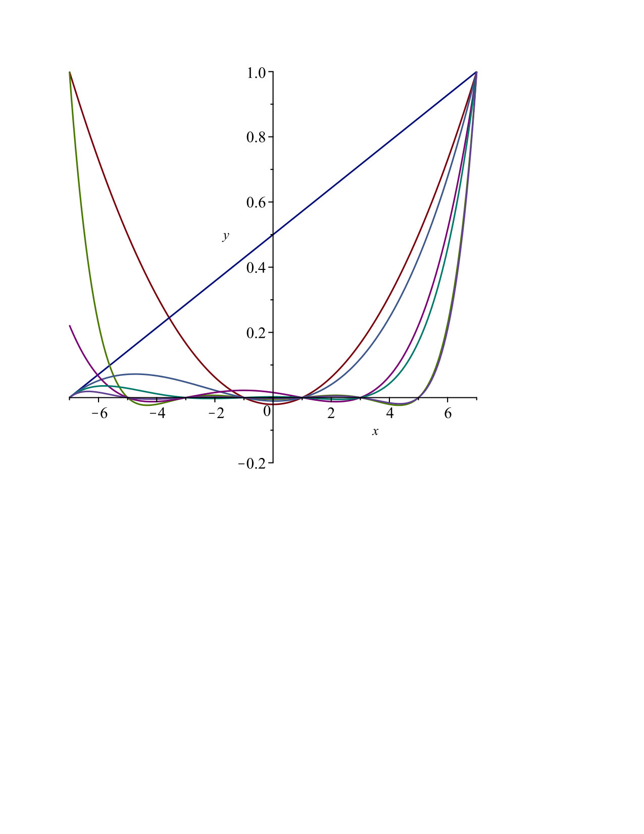 Figure 1
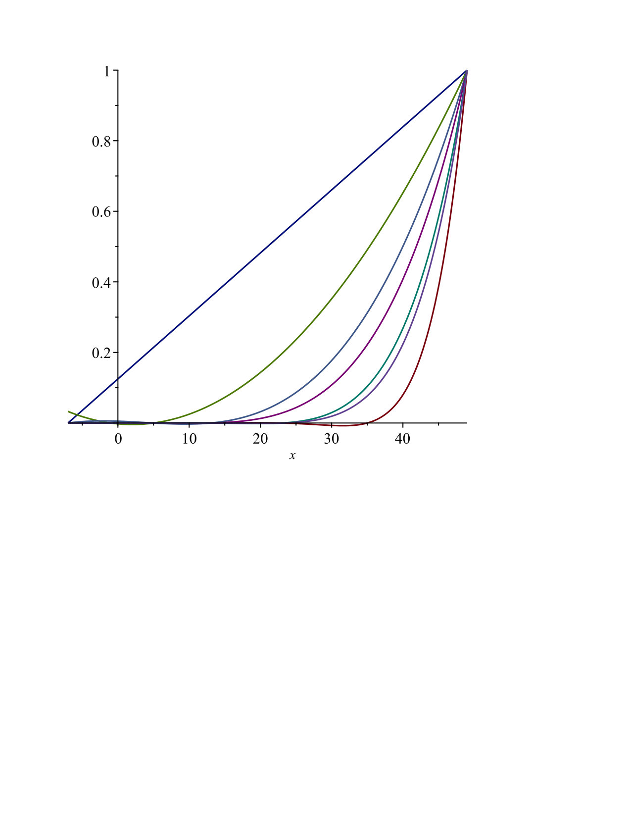 Figure 2
| 0 | 1/7 | 2/7 | 3/7 | 4/7 | 5/7 | 6/7 | 1 | |
| 1 | 1/2 | 1/6 | 0 | 0 | 1/6 | 1/2 | 1 | |
| 0 | 1/14 | 1/21 | 0 | 0 | 5/42 | 3/7 | 1 | |
| 2/9 | 0 | 0 | 1/45 | 0 | 0 | 2/9 | 1 | |
| 0 | 1/35 | 0 | 0 | 0 | 0 | 6/35 | 1 | |
| 1 | 0 | 0 | 0 | 0 | 0 | 0 | 1 | |
| 0 | 0 | 0 | 0 | 0 | 0 | 0 | 1 |
| 0 | 1/28 | 3/28 | 3/14 | 5/15 | 15/28 | 3/4 | 1 | |
| 9/275 | 1/55 | 0 | 0 | 14/275 | 54/275 | 27/55 | 1 | |
| 0 | 5/1232 | 1/176 | 0 | 0 | 75/1232 | 5/16 | 1 | |
| 1/1485 | 0 | 0 | 0 | 0 | 14/495 | 2/9 | 1 | |
| 0 | 1/2860 | 0 | 0 | 0 | 0 | 27/260 | 1 | |
| 0 | 0 | 0 | 0 | 0 | 0 | 1/13 | 1 | |
| 0 | 0 | 0 | 0 | 0 | 0 | 0 | 1 |
| graph / | ||||
|---|---|---|---|---|
| 7 | – | – | – | |
| 13 | 9 | – | – | |
| 66 | 21 | 11 | – | |
| 158 | 90 | 17 | 12 |
Peer Reviews
No public reviews on file for this paper yet. If you reviewed it on a platform where reviews are public (OpenReview, ICLR, NeurIPS, ICML), you can paste yours below so the community can read it here.
Videos
No videos yet. Explain this paper in a talk, walkthrough, or lecture? Add one.
Taxonomy
TopicsCoding theory and cryptography · graph theory and CDMA systems · Finite Group Theory Research
A new class of polynomials from the spectrum of a graph, and its application to bound the -independence number
M. A. Fiol
Departament de Matemàtiques
Universitat Politècnica de Catalunya, Barcelona, Catalonia
Barcelona Graduate School of Mathematics
Abstract
The -independence number of a graph is the maximum size of a set of vertices at pairwise distance greater than . A graph is called -partially walk-regular if the number of closed walks of a given length , rooted at a vertex , only depends on . In particular, a distance-regular graph is also -partially walk-regular for any . In this note, we introduce a new family of polynomials obtained from the spectrum of a graph. These polynomials, together with the interlacing technique, allow us to give tight spectral bounds on the -independence number of a -partially walk-regular graph. Together with some examples where the bounds are tight, we also show that the odd graph with odd has no -perfect code.
keywords: Graph, -independence number, spectrum, interlacing, minor polynomial, -partially walk-regular,
Mathematics Subject Classifications: 05C50, 05C69.
1 Introduction
Given a graph , let denote the size of the largest set of vertices such that any two vertices in the set are at distance larger than . Thus, with this notation, is just the independence number of a graph. The parameter therefore represents the largest number of vertices which can be spread out in . It is known that determining is NP-Hard in general [19].
The -independence number of a graph is directly related to other combinatorial parameters such as the average distance [12], packing chromatic number [13], injective chromatic number [17], and strong chromatic index [20]. Upper bounds on the -independence number directly give lower bounds on the corresponding distance or packing chromatic number [3], as well as necessary conditions for the existence of perfect codes.
In this note we generalize and improve the known spectral upper bounds for the -independence number from [8], [1] and [2]. For some cases, we also show that our bounds are sharp. Let be a graph with vertices, edges, and adjacency matrix with spectrum where the different eigenvalues are in decreasing order, , and the superscripts stand for their multiplicities. When the eigenvalues are presented with possible repetitions, we shall indicate them by
The first known spectral bound for the independence number of a graph is due to Cvetković [7].
Theorem 1.1** (Cvetković [7]).**
Let be a graph with eigenvalues . Then,
[TABLE]
Another well-known result is the following bound due to Hoffman (unpublished; see for instance Haemers [16]).
Theorem 1.2** (Hoffman [16]).**
If is a regular graph on vertices with eigenvalues , then
[TABLE]
Regarding the -independence number, the following three results are known. The first is due to Fiol [8] and requires a preliminary definition. Let be a graph with distinct eigenvalues . Let be chosen among all polynomials , that is, polynomials of real coefficients and degree at most , satisfying for all , and such that is maximized. The polynomial defined above is called the -alternating polynomial of and was shown to be unique in [11], where it was used to study the relationship between the spectrum of a graph and its diameter.
Theorem 1.3** (Fiol [8]).**
Let be a -regular graph on vertices, with distinct eigenvalues and let be its -alternating polynomial. Then,
[TABLE]
More recently, Cvetković-like and Hoffman-like bounds were given by Abiad, Cioabă, and Tait in [1].
Theorem 1.4** (Abiad, Cioabă, Tait [1]).**
Let be a graph on vertices with adjacency matrix , with eigenvalues . Let and be respectively the smallest and the largest diagonal entries of \mbox{\boldmathA}^{k}. Then,
[TABLE]
Theorem 1.5** (Abiad, Cioabă, Tait [1]).**
Let be a -regular graph on vertices with adjacency matrix , whose distinct eigenvalues are . Let be the largest diagonal entry of \mbox{\boldmathA}+\mbox{\boldmathA}^{2}+\cdots+\mbox{\boldmathA}^{k}. Let . Then,
[TABLE]
Finally, as a consequence of a generalization of the last two theorems, Abiad, Coutinho, and the author [2], proved the following results.
Theorem 1.6** (Abiad, Coutinho, Fiol [2]).**
Let be a -regular graph with vertices and distinct eigenvalues . Let W_{k}=W(p)=\max_{u\in V}\{\sum_{i=1}^{k}(\mbox{\boldmathA}^{k})_{uu}\}. Then, the -independence number of satisfies the following:
If , then
[TABLE]
where is the largest eigenvalue not greater than .
If is odd, then
[TABLE]
If is even, then
[TABLE]
If is a walk-regular graph, then
[TABLE]
for , where with the ’s being the predistance polynomials of (see next section), and .
2 Some Background
For basic notation and results see [4, 14]. Let be a (simple) graph with vertices, edges, and adjacency matrix with spectrum . When the eigenvalues are presented with possible repetitions, we shall indicate them by . Let us consider the scalar product in :
[TABLE]
The so-called predistance polynomials are a sequence of orthogonal polynomials with respect to the above product, with , and they are normalized in such a way that (this makes sense since it is known that ) for . Therefore they are uniquely determined, for instance, following the Gram-Schmidt process. These polynomials were introduced by Fiol and Garriga in [10] to prove the so-called ‘spectral excess theorem’ for distance-regular graphs, where coincide with the so-called distance polynomials . See [6] for further details and applications.
A graph is called -partially walk-regular, for some integer , if the number of closed walks of a given length , rooted at a vertex , only depends on . Thus, every (simple) graph is -partially walk-regular for , and every regular graph is -partially walk-regular. Moreover is -partially walk-regular for any if and only if is walk-regular, a concept introduced by Godsil and Mckay in [15]. For example, it is well-known that every distance-regular graph is walk-regular (but the converse does not hold).
Eigenvalue interlacing is a powerful and old technique that has found countless applications in combinatorics and other fields. This technique will be used in several of our proofs. For more details, historical remarks, and other applications, see Fiol and Haemers [9, 16]. Given square matrices and with respective eigenvalues and , with , we say that the second sequence interlaces the first one if, for all , it follows that .
Theorem 2.1** (Interlacing [9, 16]).**
Let be a real matrix such that \mbox{\boldmathS}^{T}\mbox{\boldmathS}=\mbox{\boldmathI}, and let be a matrix with eigenvalues . Define \mbox{\boldmathB}=\mbox{\boldmathS}^{T}\mbox{\boldmathA}\mbox{\boldmathS}, and call its eigenvalues . Then,
- (i)
The eigenvalues of interlace those of . 2. (ii)
If or , then there is an eigenvector of for such that * is eigenvector of for .* 3. (iii)
If there is an integer such that for , and for tight interlacing, then \mbox{\boldmathS}\mbox{\boldmathB}=\mbox{\boldmathA}\mbox{\boldmathS}.
Two interesting particular cases where interlacing occurs (obtained by choosing appropriately the matrix ) are the following. Let be the adjacency matrix of a graph . First, if is a principal submatrix of , then corresponds to the adjacency matrix of an induced subgraph of . Second, when, for a given partition of the vertices of , say , is the so-called quotient matrix of , with elements , , being the average row sums of the corresponding block \mbox{\boldmathA}_{ij} of . Actually, the quotient matrix does not need to be symmetric or equal to \mbox{\boldmathS}^{\top}\mbox{\boldmathA}\mbox{\boldmathS}, but in this case is similar to (and therefore has the same spectrum as) \mbox{\boldmathS}^{\top}\mbox{\boldmathA}\mbox{\boldmathS}.
3 The minor polynomials
In this section we introduce a new class of polynomials, obtained from the different eigenvalues of a graph, which are used later to derive our main results.
Let be a -partially walk-regular graph with adjacency matrix and spectrum . Let be a polynomial of degree at most , satisfying and for . Then, in Section 4 we prove that has -independence number satisfying the bound \alpha_{k}\leq\mathop{\rm tr}\nolimits p_{k}(\mbox{\boldmathA})=\sum_{i=0}^{d}m_{i}p_{k}(\theta_{i}). So, the search for the best result motivates the following definition.
Definition 3.1**.**
Let be a graph with adjacency matrix with spectrum . For a given , let us consider the set of real polynomials , and the continuous function defined by \Psi(p)=\mathop{\rm tr}\nolimits p(\mbox{\boldmathA}). Then, the -minor polynomial of is the point where attains its minimum:
[TABLE]
An alternative approach to the -minor polynomials is the following: Let be the polynomial defined by and , for , where the vector is a solution of the following linear programming problem:
\begin{array}[]{rl}&\\ {\tt minimize}&\sum_{i=0}^{d}m_{i}x_{i}\\ {\tt with\ constraints}&f[\theta_{0},\ldots,\theta_{m}]=0,\ m=k+1,\ldots,d\\ &x_{i}\geq 0,\ i=1,\ldots,d,\\ &\end{array}
where denote the -th divided differences of Newton interpolation, recursively defined by , where , starting with , .
Thus, we can easily compute the minor polynomial, for instance by using the simplex method. Moreover, as the problem is in the so-called standard form, with variables, , and equations, the ‘basic vectors’ have at least zeros. Note also that, from the conditions of the programming problem, the -minor polynomial turns out to be of the form , with degree at most . Consequently when we apply the simplex method, we obtain a -minor polynomial with degree and exactly zeros at the mesh . In fact, as shown in the following lemma, a -minor polynomial has exactly zeros in the interval .
Proposition 3.2**.**
Let be a graph with spectrum . Then, for every , a -minor polynomial has degree with its zeros in .
Proof.
We only need to deal with the case . Assume that a -minor polynomial has the zeros with . Then, it can be written as . Let us first show that . By contradiction, assume that , and let the smallest eigenvalue which is not a zero of (the existence of such a is guaranteed from the condition ). Then, the polynomial , with degree satisfies the conditions , for , and since for , a contradiction with the fact that is minimum. Second, let us prove, again by contradiction, that . Otherwise, we could consider the polynomial , with degree , defined as satisfying again , and for since for all . But, from the same inequalities, we also have , a contradiction.
Finally, assume that . Since all zeros are in the interval , we can consider again the smallest one such that . Then, reasoning as before, the polynomial , with degree leads to the desired contradiction . ∎
The above results, together with and for drastically reduce the number of possible candidates for . Let us consider some particular values of :
- •
The cases and are easy. Clearly, , and has zeros at all the points for . In fact, , where is the Hoffman polynomial [18].
- •
For , the only zero of must be at . Hence,
[TABLE]
Moreover, since for every , we have that
[TABLE]
since, for , for every .
- •
For , the two zeros of must be at consecutive eigenvalues and . More precisely, the same reasonings used in [2] shows that must be the largest eigenvalue not greater than . Then, with these values,
[TABLE]
- •
When , the only possible zeros of are and the consecutive pair , for some . In this case, empirical results seem to point out that such a pair must be around the ‘center’ of the mesh (see the examples below).
- •
When , the polynomial takes only one non-zero value at the mesh, say at , which seems to be located at one of the ‘extremes’ of the mesh. In fact, when is an -antipodal distance-regular graph, we show in the last section that either or for odd yields the tight bound (that is, ) for , as does Theorem 1.3. Consequently, for such a graph with odd , we have two different -minor polynomials, say and , and hence infinitely many -minor polynomials of the form where . (Notice that, if , then must have some zero not belonging to the mesh .)
Now, let us give all the -minor polynomials, with , for two particular distance-regular graphs. Namely, the Hamming graph and the Johnson graph (for more details about these graphs, see for instance [5]). First, we recall that the Hamming graph has spectrum
[TABLE]
Then, the different minor polynomials are shown in Figure 1, and their values at the different eigenvalues are shown in Table 1.
As another example, consider the the Johnson graph (see, for instance, [5, 14]). This is an antipodal (but not bipartite) distance-regular graph, with vertices, diameter , and spectrum
[TABLE]
Then the solutions of the linear programming problem are in Table 2, which correspond to the minor polynomials shown in Figure 2
4 A tight bound for the -independence number
Now we are ready to derive our main result about the -independent number of a -partially walk-regular graph. The proof is based on the interlacing technique.
Theorem 4.1**.**
Let be a -partially walk-regular graph with vertices, adjacency matrix , and spectrum . Let be a -minor polynomial. Then, for every , the -independence number of satisfies
[TABLE]
Proof.
Let be a -independent set of with vertices. Again, assume the first columns (and rows) of correspond to the vertices in . Consider the partition of said columns according to and its complement. Let be the normalized characteristic matrix of this partition. The quotient matrix of p(\mbox{\boldmathA}) with regards to this partition is given by
[TABLE]
with eigenvalues and
[TABLE]
where . Then, by interlacing, we have
[TABLE]
whence, solving for , we get and the result follows. ∎
As mentioned in the previous section, notice that, in fact, the proof works for any polynomial satisfying and for . By way of example, if is a distance-regular graph with distance polynomials , we could take , with degree , where the sum polynomial satisfies . Now, recall that corresponds to the number of vertices at distance from any vertex of (see, for instance Biggs [4]). Thus, we obtain
[TABLE]
as expected.
Another possibility is to use the polynomial , where is the -alternating polynomial. In this case, when is an -antipodal distance-regular graphs and , it turns out that the -distance polynomial is , where is the Hoffman polynomial (see [8]). Then, we get , which coincides with the bound for given in Theorem 1.3.
Let us now consider some particular cases of Theorem 4.1 by using the minor polynomials.
The case .
As mentioned above, coincides with the standard independence number . In this case the minor polynomial is . Then, (3) gives
[TABLE]
which is Hoffman’s bound in Theorem 1.2.
The case .
We already stated that . Then, (3) yields
[TABLE]
in agreement with the result of [2] (here in Theorem ). Moreover, in the same paper, two infinite families of (distance-regular) graphs where the bound (12) is tight were provided.
Some examples
To compare the above bounds with those obtained in [8] and [1] (here in Theorems 1.3 and 1.5, respectively), let us consider again the Hamming graph and the Johnson graph . Thus, in Table 3 we show the bounds obtained for , whereas those of are shown in Table 5. (Recall that every distance-regular graph is also walk-regular.)
Note that, in general, the bounds obtained by Theorem 4.1 constitute a significant improvement with respect to those in [8, 1]. In particular, the bounds for are equal to the correct values (since both graphs are -antipodal), and (since their diameter is ). Besides notice that, in the case of the Hamming graph, since it contains the perfect Hamming code .
4.1 Antipodal distance-regular graphs
Finally, we consider an infinite family where our bound for is tight. With this aim, we assume that the minor polynomial takes non-zero value only at . Thus, . Then, the bound (3) of Theorem 4.1 is
[TABLE]
where, in general, for . Now suppose that is an -antipodal distance-regular graph. Then, in [8] it was shown that is so if and only if its eigenvalue multiplicities are for even, and for odd. So, with , we get
[TABLE]
which is the correct value.
When is an -antipodal distance-regular graph with odd , we can also consider the minor polynomial which takes non-zero value only at , that is . Then, reasoning as above, we get again the tight bound .
4.2 Odd graphs
For every integer , the odd graphs constitute a well-known family of distance-regular graphs with interactions between graph theory and other areas of combinatorics, such as coding theory and design theory. The vertices of correspond to the -subsets of a -set, and adjacency is defined by void intersection. In particular, is the Petersen graph. In general, the odd is a -regular graph with order , diameter , and its eigenvalues and multiplicities are and for . For more details, see for instance, Biggs [4] and Godsil [14].
In Table 5 we show the bounds of the -independence numbers for , given by Theorem 4.1. The numbers in bold faces, and , correspond to the known -perfect codes in and , respectively.
More generally, (11) and (12) allow us to compute the bounds for and of every odd graph , which turn out to be
[TABLE]
where we have indicated their asymptotic behaviour, when , by using the Stirling’s formula. As a consequence, we have the known result that, when is odd, the odd graph has no -perfect code. Indeed, the existence of -perfect code in requires that (since all codewords must be mutually at distance ). However, when is odd, (14) gives , a contradiction. (In fact, when is a power of two minus one is not an integer, which also prevents the existence of a -perfect code.) Note that this result is in agreement with the fact that a necessary condition for a regular graph to have a -perfect code is the exitence of the eigenvalue , which is not present in when is odd (see Godsil [14]).
Finally, by using the same polynomial as in Subsection 4.1, we have that the -independence number of , where , satisfies the bounds
[TABLE]
For instance, for the Petersen graph , this yields , as it is well-known.
Acknowledgments
This research has been partially supported by AGAUR from the Catalan Government under project 2017SGR1087, and by MICINN from the Spanish Government under project PGC2018-095471-B-I00.
The reference list from the paper itself. Each links out to its DOI / PubMed record.
- 1[1] A. Abiad, S. M. Cioabă, and M. Tait, Spectral bounds for the k 𝑘 k -independence number of a graph, Linear Algebra Appl. 510 (2016) 160–170.
- 2[2] A. Abiad, G. Coutinho, and M. A. Fiol, On the k 𝑘 k -independence number of graphs, Discrete Math. , 342 (2019), no. 10, 2875–2885.
- 3[3] N. Alon and B. Mohar, The chromatic number of graph powers, Combin. Probab. Comput. 11(1) (2002) 1–10.
- 4[4] N. Biggs, Algebraic Graph Theory , Cambridge University Press, Cambridge, 1974, second edition, 1993.
- 5[5] A. E. Brouwer, A. M. Cohen, and A. Neumaier, Distance-Regular Graphs , Springer, Heidelberg, 1989.
- 6[6] M. Cámara, J. Fàbrega, M. A. Fiol, and E. Garriga, Some families of orthogonal polynomials of a discrete variable and their applications to graphs and codes, Electron. J. Combin. 16 (2009) #R 83.
- 7[7] D. M. Cvetković, Graphs and their spectra, Publ. Elektrotehn. Fak. Ser. Mut. Fiz. 354-356 (1971) 1–50.
- 8[8] M. A. Fiol, An eigenvalue characterization of antipodal distance-regular graphs, Electron. J. Combin. 4(1) (1997) #R 30.