QPROP with faster calculation of photoelectron spectra
Vasily Tulsky, Dieter Bauer

TL;DR
This paper introduces QPROP 3.0, an improved computational tool for calculating photoelectron spectra more efficiently using the i-SURFV method, reducing post-processing time in strong-field laser-atom simulations.
Contribution
QPROP 3.0 incorporates the novel i-SURFV method for single-step post-propagation, enhancing the efficiency of photoelectron spectra calculations in strong-field physics.
Findings
i-SURFV reduces post-propagation computational time.
Enhanced parameter handling improves user experience.
Examples demonstrate the efficiency of the new method.
Abstract
The calculation of accurate photoelectron spectra (PES) for strong-field laser-atom experiments is a demanding computational task, even in single-active-electron approximation. The QPROP code, published in 2006, has been extended in 2016 in order to provide the possibility to calculate PES using the so-called t-SURFF approach [L. Tao, A. Scrinzi, New J. Phys. 14, 013021 (2012)]. In t-SURFF, the flux through a surface while the laser is on is monitored. Calculating PES from this flux through a surface enclosing a relatively small computational grid is much more efficient than calculating it from the widely spread wavefunction at the end of the laser pulse on a much larger grid. However, the smaller the minimum photoelectron energy of interest is, the more post-propagation after the actual laser pulse is necessary. This drawback of t-SURFF has been overcome by Morales et al. [F. Morales,…
Click any figure to enlarge with its caption.
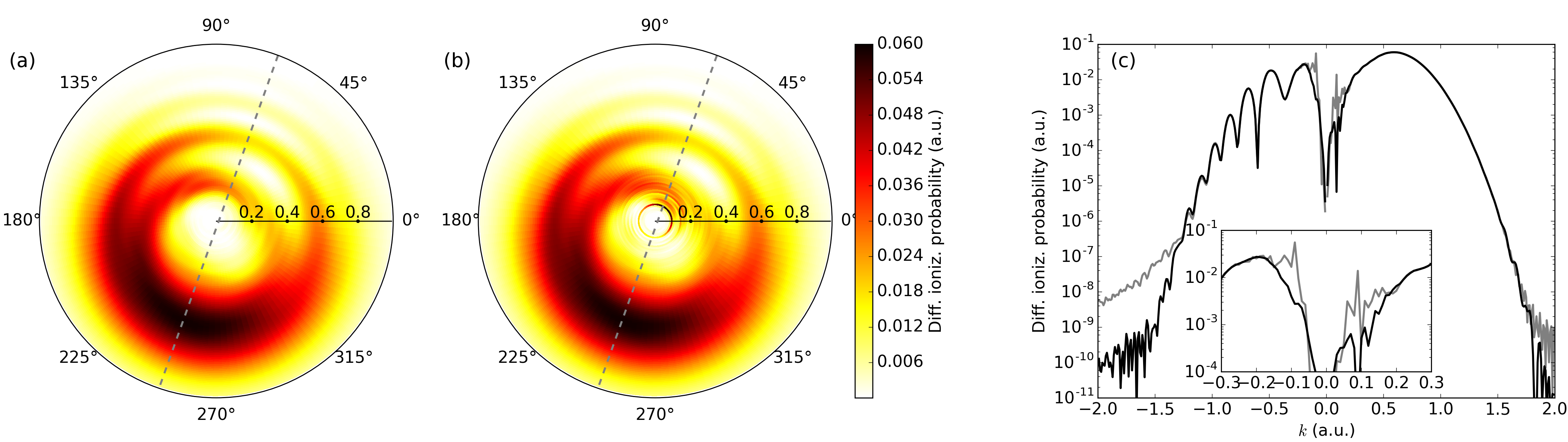 Figure 1
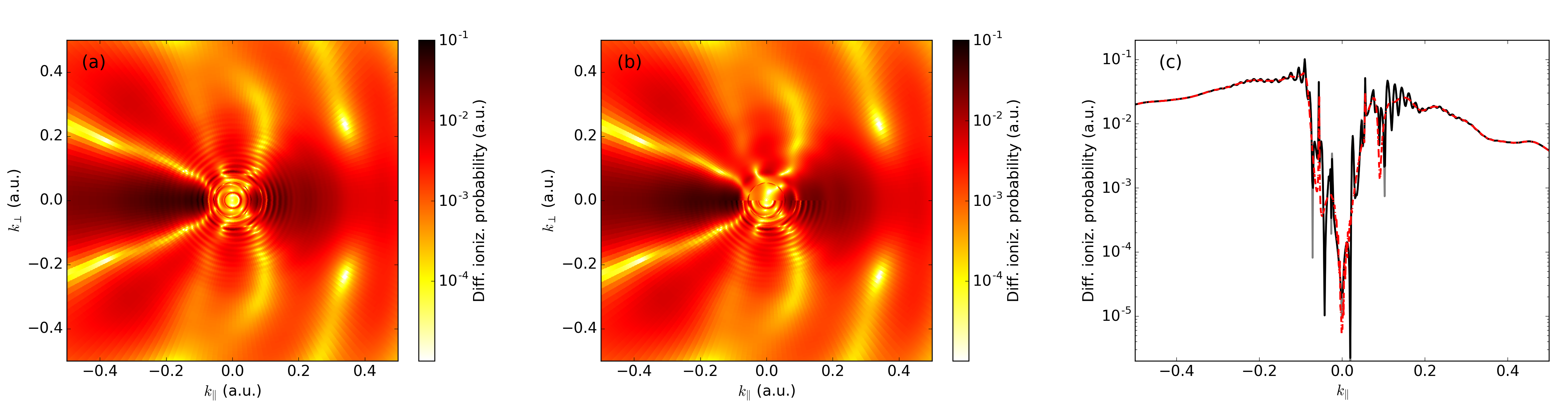 Figure 2
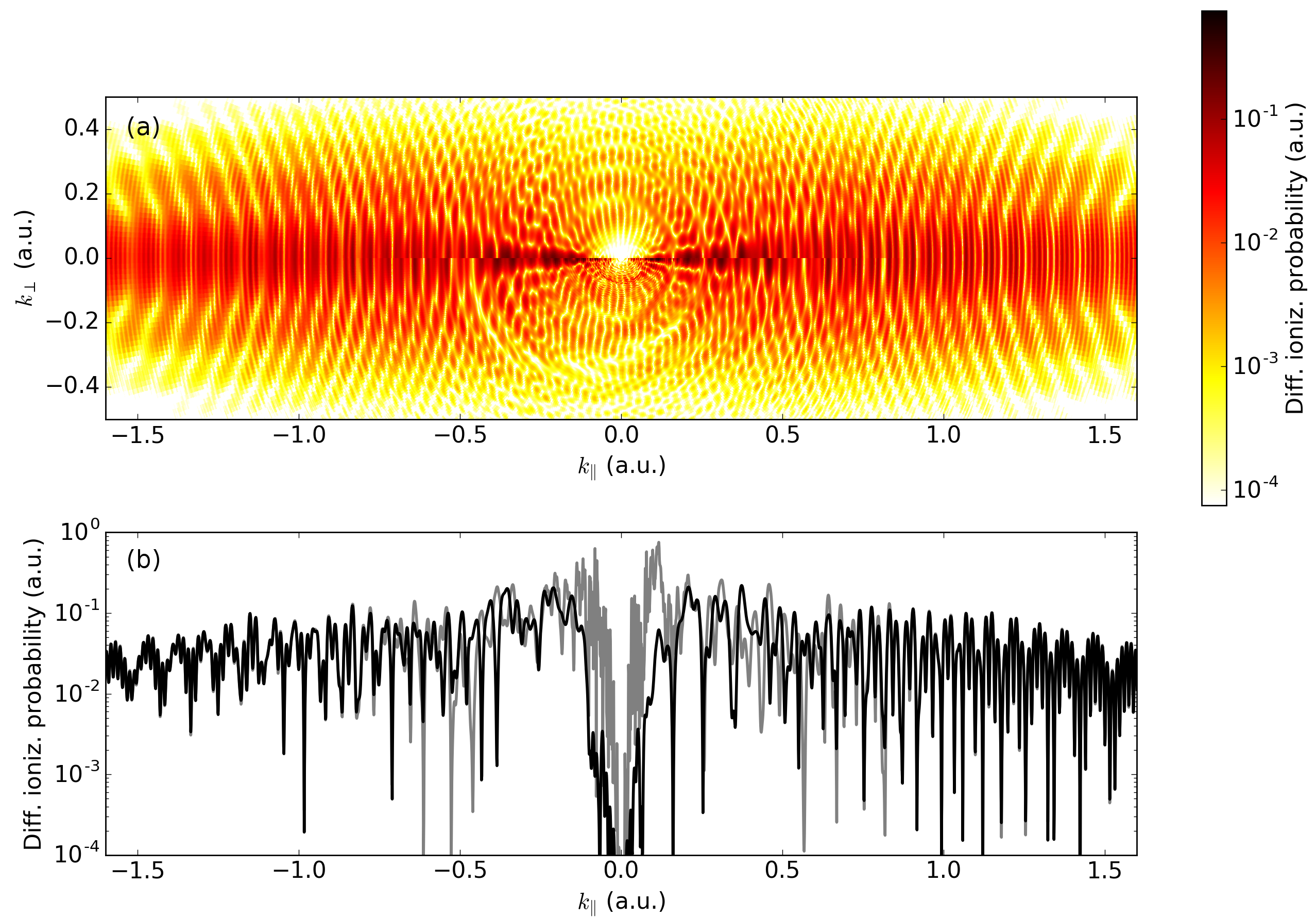 Figure 3
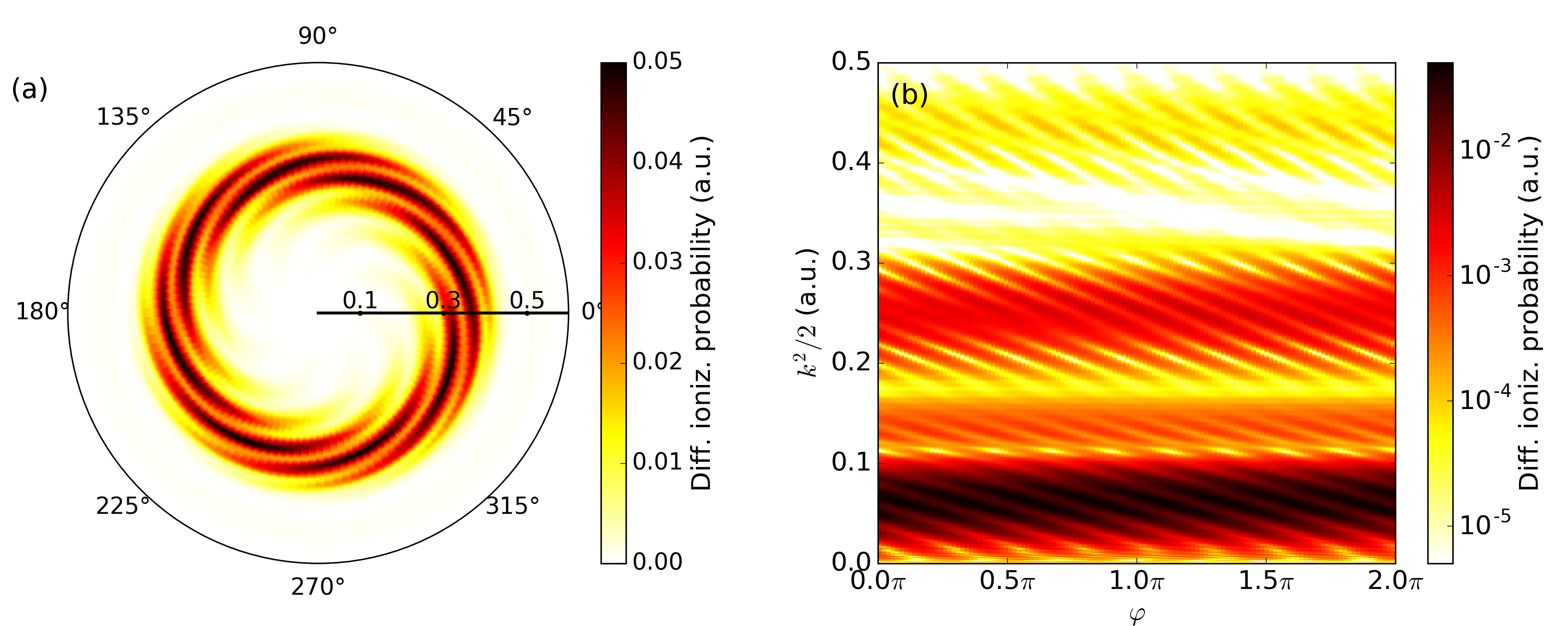 Figure 4
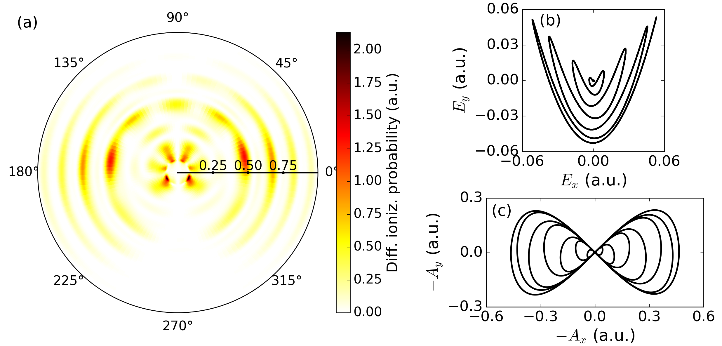 Figure 5
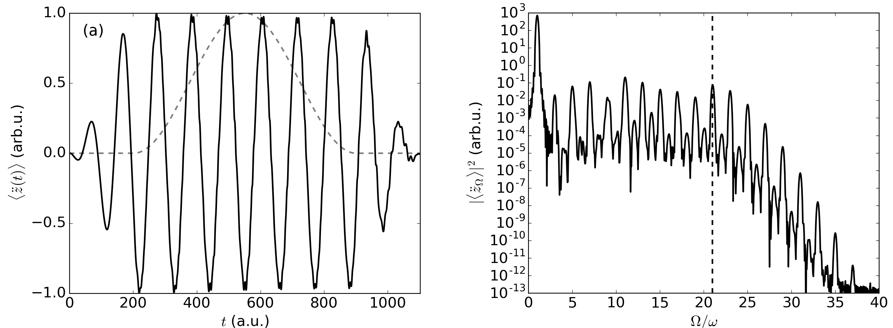 Figure 6
| Qprop 2.0 | Qprop 3.0 | Task |
| hydrogen_im | imag_prop | Imaginary-time propagation |
| hydrogen_re | real_prop | Real-time propagation |
| isurfv | to , | |
| eval-tsurff(-mpi) | tsurff(_mpi) | Spectrum with t-SURFF |
| Parameter | Eq. (4.2) | Domain | Default in | |
|---|---|---|---|---|
| vortex | lissajous | |||
| omega-1 | ||||
| omega-2 | ||||
| max-electric-field-1-x | ||||
| max-electric-field-2-x | ||||
| max-electric-field-1-y | ||||
| max-electric-field-2-y | ||||
| num-cycles-1 | ||||
| num-cycles-2 | ||||
| phase-1-x | ||||
| phase-2-x | ||||
| phase-1-y | ||||
| phase-2-y | ||||
| tau-delay | ||||
Peer Reviews
No public reviews on file for this paper yet. If you reviewed it on a platform where reviews are public (OpenReview, ICLR, NeurIPS, ICML), you can paste yours below so the community can read it here.
Videos
No videos yet. Explain this paper in a talk, walkthrough, or lecture? Add one.
Qprop with faster calculation of photoelectron spectra
Vasily Tulsky
Dieter Bauer
Institut für Physik, Universität Rostock, 18051 Rostock, Germany
Abstract
The calculation of accurate photoelectron spectra (PES) for strong-field laser-atom experiments is a demanding computational task, even in single-active-electron approximation. The Qprop code, published in 2006, has been extended in 2016 in order to provide the possibility to calculate PES using the so-called t-SURFF approach [L. Tao, A. Scrinzi, New J. Phys. 14, 013021 (2012)]. In t-SURFF, the flux through a surface while the laser is on is monitored. Calculating PES from this flux through a surface enclosing a relatively small computational grid is much more efficient than calculating it from the widely spread wavefunction at the end of the laser pulse on a much larger grid. However, the smaller the minimum photoelectron energy of interest is, the more post-propagation after the actual laser pulse is necessary. This drawback of t-SURFF has been overcome by Morales et al. [F. Morales, T. Bredtmann, S. Patchkovskii, J. Phys. B: At. Mol. Opt. Phys. 49, 245001 (2016)] by noticing that the propagation of the wavefunction from the end of the laser pulse to infinity can be performed very efficiently in a single step. In this work, we introduce Qprop 3.0, in which this single-step post-propagation (dubbed i-SURFV) is added. Examples, illustrating the new feature, are discussed. A few other improvements, concerning mainly the parameter files, are also explained.
keywords:
Time-dependent Schrödinger equation , strong-field ionization , photoelectron spectra , time-dependent surface flux method , two-color fields
††journal: Computer Physics Communications
NEW VERSION PROGRAM SUMMARY
Manuscript Title: Qprop with faster calculation of photoelectron spectra
Authors: Vasily Tulsky, Dieter Bauer
Program Title: Qprop
Journal Reference:
*Catalogue identifier:
Licensing provisions:* GNU General Public License, version 3
Programming language: C++
Computer: x86_64
Operating system: Linux
RAM: The memory requirement depends on the desired resolution of the photoelectron spectrum: examples provided with the package need about 1 GB of RAM (with the exception long-wavelength that needs 3.5GB of RAM). If no photoelectron spectrum is produced (hhg example) then only a few MB are necessary.
Number of processors used: Calculation of PES supports parallelization on up to processes equal to the number of radial momenta of interest.
Keywords: Time-dependent Schrödinger equation, strong-field ionization, photoelectron spectrum, time-dependent surface flux method, two-color fields.
*External routines/libraries: * GNU Scientific Library, Open MPI (optional).
Catalogue identifier of previous version: ADXB_v2_0
Journal reference of previous version: Comput. Phys. Comm. 207(2016) 452-463
Does the new version supersede the previous version?: Fully supports the functionality of Qprop 2.0.
Nature of problem: Efficient calculation of PES for typical strong-field and attosecond physics ionization scenarios.
Solution method: The time-dependent Schrödinger equation is solved by propagating the electronic wavefunction using a Crank-Nicolson propagator. The wavefunction is represented by an expansion in spherical harmonics. The t-SURFF method in combination with i-SURFV is used to calculate PES.
Reasons for the new version: The i-SURFV method is employed to speed up the calculation of PES.
Summary of revisions: The i-SURFV method is implemented. A set of examples is provided.
Restrictions: The atomic potential needs to be of finite range in case of t-SURFF/i-SURFV usage (i.e., the Coulomb tail is truncated at sufficiently large distances). The laser-matter interaction is described in dipole approximation and velocity gauge.
Additional comments: For additional information see www.qprop.de
Running time: Depends on the laser configuration and on the resolution of PES. Most examples require between 7 to 35 minutes. The longest needs about 1.5 hours.
1 Introduction
Intense-laser-matter experiments brought forward many surprising results that were inaccessible to conventional perturbative theoretical approaches (see, e.g., [1]). As a consequence, new but less rigorous or semi-classical methods have been developed [2, 3, 4, 5] that, however, need to be tested against numerical ab initio solutions. Already the solution of the time-dependent Schrödinger equation (TDSE) for a single active electron in an effective atomic potential and in the presence of a classical, strong laser field can be a demanding computational task [6, 7, 8, 9].
The present paper is devoted to a revised version of Qprop — a position-space TDSE-solver for a single active electron bound in a spherically symmetric potential and subject to an external, time-dependent, space-homogeneous electric field (representing the laser field in dipole approximation). Qprop was introduced in Ref. [7]. A revised version of Qprop employing the time-dependent surface flux method (t-SURFF) for the calculation of PES as proposed in Ref. [10] was published in Ref. [9]. Using t-SURFF, the PES are calculated from the probability flux through a surface located sufficiently far away from the effective range of the binding potential. The time interval over which the flux is captured is limited by the simulation time. Hence, those components of the electronic wavefunction that represent the slowest electrons of interest should reach the t-SURFF surface during the simulation time. In practice, that means that the simulation time might be many times the actual laser pulse duration, in particular for the simulation of ultra-short pulse experiments. In this paper, we introduce Qprop 3.0, where this post-pulse propagation just to capture the slow electrons is avoided using the “trick” proposed in [8] called i-SURFV: once the laser field is off, the evolution of the system is described by a time-independent Hamiltonian, and the contribution to the surface flux after the pulse up to infinity can be calculated in a single step. Refining the formulas used in Qprop 2.0 [9], it is possible to reduce this evaluation to an action of a non-local operator.
The paper is organized as follows. Section 2 contains the mathematical formulation of the upgraded version of t-SURFF (i.e., i-SURFV) that is implemented in Qprop 3.0. In Section 3, the most important functions and data structures are described. Section 4 contains examples. Two examples were already in the Qprop 2.0 paper [9], thus demonstrating nicely the improvement in performance using i-SURFV. A few more demo configurations that may serve as useful templates for a user have been added.
Atomic units are used throughout the paper unless other units are explicitly given.
2 Theoretical basis for i-SURFV
2.1 Hamiltonian and wavefunction
We consider a single active electron, initially bound by the atomic potential, under the influence of a laser field. This system is described by the TDSE
[TABLE]
with the Hamiltonian in velocity gauge
[TABLE]
Here, is the binding potential of the atom, is the vector potential in dipole approximation (i.e., the electric field is ), and is the imaginary potential which plays the role of an absorber to exclude unphysical reflections in the wavefunction off the numerical boundary. The purely time-dependent term (that arises from the minimum coupling term ) has been transformed away. Due to the spherical symmetry of the potential , it is convenient to expand the wavefunction in spherical harmonics,
[TABLE]
The upper limit for the orbital angular momentum quantum number is finite in numerical calculations, i.e.,
[TABLE]
is defined by the user. If the polarization of the laser is chosen linear along the axis and the magnetic quantum number of the initial state is well defined, is conserved during time propagation so that only contributes to the sum over ,
[TABLE]
We discretize time and the radial coordinate in units of and , respectively. The radial grid is of size where is the position of the flux-capturing surface for t-SURFF, is the quiver amplitude in the chosen laser field of electric field maximum , and is the width of the imaginary potential that has the form
[TABLE]
with , and by default. The spherically symmetric potential can be defined by the user. In the following, we use a potential of the residual atom that is hydrogenic but is switched to linear at and is off after reaching zero at :
[TABLE]
The cutoff radius is defined by the user in the initial.param file. The t-SURFF/i-SURFV method for the calculation of PES requires that . The shapes of the binding and imaginary potentials are defined in potentials.hh.
2.2 t-SURFF and i-SURFV
Before we move on to the i-SURFV method, let us briefly review the basics of t-SURFF [10] (see [9] for t-SURFF in the context of Qprop). The PES amplitudes at time after the laser pulse are approximated in t-SURFF by projecting the part of the wavefunction that is farther away from the origin than onto Volkov states of the momentum of interest ,
[TABLE]
Volkov states are plane-wave states in the presence of a laser field [11, 4]. is chosen such that the potential and, hence, the bound states in the region beyond are irrelevant for the effect studied. The time should be large enough such that an electron with the smallest momentum of interest arrives at the t-SURFF boundary , i.e., . The amplitude (8) can be rewritten in the form of a time integral
[TABLE]
The second term vanishes, as with a properly chosen the initial wavefunction is negligible for . Using the TDSE (1) for and for , where coincides with in the region , the remaining term can be written as
[TABLE]
At this point, let us split the integral over time into parts before and after the end of the laser pulse ,
[TABLE]
The first term is treated in Qprop numerically as it was described in [9] while the second, field-free term can be calculated without expensive post-propagation of the wavefunction after the laser pulse. This avoidance of post-propagation up to the time where the slowest electrons of interest passed the t-SURFF boundary is the essence of i-SURFV as proposed in Ref. [8] and the core advantage of the new version of Qprop 3.0 over version 2.0.
Let us rewrite the field-free part in the matrix element (11) as
[TABLE]
with and . Integrating the last term by parts, we obtain
[TABLE]
The (complex conjugated) plane-wave final-momentum state in position space at times can be expressed as
[TABLE]
where are spherical Bessel functions, and is represented as (4) or (5). Expanding
[TABLE]
one finds
[TABLE]
with . The formula is used in the program code to calculate the derivatives of the spherical Bessel functions.
The time integral can be evaluated in the limit using the explicit form of the time evolution operator,
[TABLE]
where the time-independent Hamiltonian has the form
[TABLE]
The operator is the Green’s function for the radial Schrödinger equation, i.e., the energy representation of the solution to
[TABLE]
The related function in the i-SURFV code is thus named gfunc. The contribution of the upper limit in (17) vanishes due to the presence of an absorbing, imaginary potential. The final expression for the field-free part of the full amplitude can be thus written as
[TABLE]
where . The integral over an infinite time has been converted to a single application of the operator (per and ), which is the essence of the infinite-time version of t-SURFF, i.e., i-SURFV. How the application of such an inverse operator is actually implemented needs not to be detailed here, as it is similar to the application of the spectral window operator explained in detail in [7]. The applicability of the i-SURFV “trick” is discussed in section 4 by several example configurations included in the Qprop 3.0 distribution.
3 Qprop** general structure**
Parameters and flags
In the current version, all parameters defining coordinate, momentum, and time grids, the potentials, and the laser are moved to the *param files. Most of the flags that allow to switch between different methods or to turn on and off the generation or the storage of specific output are also put into those files. Thus, it is no longer necessary to touch *.cc files for a wide range of problems. All parameters and flags are commented so that their function should become very clear while going through the examples in section 4.
Functions and classes
The core parts of the current Qprop version are as follows.
The real or imaginary time propagation by a single timestep is performed in the member function propagate of class wavefunction, which is described in the first Qprop paper [7].
- 2.
The class tsurffSaveWF was designed for saving and required for t-SURFF. For i-SURFV, an additional class tsurffSave_full_WF saving was added. The data files end with *.raw.
- 3.
The Green’s function (17) is applied in gfunc, calculating and from for given .
- 4.
The calculation of a PES using t-SURFF and i-SURFV is performed with the help of the class tsurffSpectrum.
Surface flux output format
In the Qprop 2.0 paper [9], two possible expansions of the amplitudes were introduced. If the expansion in angles (according eq. (21) in [9]) is chosen, the data generated by tsurffSpectrum ((29) in [9]) in the output files tsurff_polar.dat111Here, refers to the index of the process that generated the file ( if the non-parallelized version is used). is formatted as
[TABLE]
.
For a linearly polarized laser pulse along the axis, the spectrum does not depend on the azimuthal angle , and the calculation is performed for only. For a laser pulse polarized in the plane, the user might be solely interested in the spectrum in the polarization plane. For that purpose, only data for is generated if is chosen.
If a “complete” expansion in spherical harmonics ((30) in [9]) is desired, data with partial amplitudes according eq. (35) in [9] are stored in tsurff_partial.dat files in the format
[TABLE]
where with in the case of expansion (5), and with in the general case (4).
One should note that the complete expansion involves the calculation of Clebsch-Gordan coefficients in terms of Wigner 3 symbols, which are evaluated using the GNU Scientific Library (GSL). However, the respective GSL routine gsl_sf_coupling_3j appears to have acceptable precision only for relatively small ( see, e.g., Fig. 1 in [12]). Nevertheless, for small the complete expansion can be used to identify dominating angular momenta as a function of energy.
Complexity scaling
The main steps that are required for the calculation of PES with Qprop scale as follows with respect to the number of timesteps, radial grid points, orbital momenta, photoelectron energies and angles:
Imaginary-time propagation:
- 2.
Real-time propagation:
- 3.
t-SURFF or i-SURFV:
- 4.
Green’s function “trick” for i-SURFV:
4 Examples
The quickest way to run an example is to go to its folder and launch the do_all bash script by typing ./do_all.sh in the terminal. Alternatively, one may make and execute the programs for imaginary time propagation (imag_prop), real-time propagation (real_prop) and t-SURFF (tsurff or tsurff_mpi for an MPI-parallelized version) manually. These programs have been slightly revised and renamed in Qprop 3.0. Table 1 shows the old program names in Qprop 2.0, the new names in Qprop 3.0, together with the program task. The user may edit the tsurff.param file and set the variable tsurff-version equal to 1 for t-SURFF or equal to 2 for i-SURFV. If i-SURFV is chosen, it is required to make and execute isurfv after the real-time propagation (this step is included in ./do_all.sh). This generates the data used to calculate the laser-free contribution to the PES according to eq. (2.2). Already in Qprop 2.0, half a Hanning window
[TABLE]
was by default multiplied to the integrand for the interval of the time integral (13). We keep this feature in Qprop 3.0 if t-SURFF is used.
All parameters defining the -grid, the laser pulse and the momentum grid for the PES are defined in the *.param files. Their precise meaning can be found in the comments there.
All plots shown in this paper were produced using Python scripts that are provided with Qprop 3.0. A brief guide to them can be found at the end of the paper in section 5.
4.1 Speeding up a previous Qprop 2.0 example
Time222For this and other examples, the estimated run times are calculated according [imag_prop + real_prop + isurfv time] + ([tsurff_mpi average time] 4 processes used) if the i-SURFV method is used. The compilation time is not counted. Calculations are performed on a desktop PC with Intel(R) Core(TM) i5-6500 CPU.: 6 min + (1 min 4).
Memory333The maximum RAM space required is determined by the surface flux that needs to be loaded to calculate the PES with t-SURFF. For the default parameters it is 16 bytes 4 (or 3 in the linear-polarization case) .: 229 MB 4.
In the previous Qprop version, t-SURFF required lengthy post-propagation in real time after the laser pulse is over in order to obtain the yield at low momenta. The time interval necessary to capture the PES down to momentum was estimated as . In contrast, the i-SURFV real-time propagation up to the end of the pulse plus one additional step covering is independent of the lowest momentum of interest. The difference between the total calculation times for the “old” t-SURFF and the new i-SURFV is especially pronounced for short pulses, which are, in fact, often used in modern experiments. To demonstrate this, we revisit an example from Qprop 2.0 [9]: a hydrogen atom in a very short ( cycles) circularly polarized pulse444Note that in the new version of Qprop linear or circular laser polarizations are chosen in initial.param where the value of qprop-dim is set to for linear polarization (along axis) or for circular polarization (in plane). No .cc source files need to be modified anymore. with ( nm), ( Wcm-2*) described by the vector potential (the shape of which is defined in potentials.hh),
[TABLE]
The corresponding folder is named attoclock, eponymous to the experiments with such pulses [13]. Compare Fig. 1(a) with Fig. 1(b) that represent the results obtained with t-SURFF and i-SURFV, respectively. The real-time propagation for i-SURFV is equal to the pulse duration and takes 2205 timesteps. It is significantly smaller than the total time required for t-SURFF with , which takes 22205 timesteps. Fig. 1(c) shows the spectra cut along (and , represented by negative values). A discrepancy on the logarithmic scale is visible in the high-energy region close to the noise level. This could be improved by increasing the values for and , i.e., R-tsurff and imag-width in propagate.param. The low-energy part of the i-SURFV spectrum has a ring-shaped, sharp peak. This artifact is not caused by i-SURFV and would appear in t-SURFF as well if a longer laser-free post-propagation were performed (i.e., if a smaller were chosen). The origin of this structure is the truncation of the potential, and it can be shifted to even lower energies by increasing the cutoff radius (i.e., pot-cutoff in initial.param) or by choosing a smoother potential shape in the intermediate domain . As noted above, the potential should vanish at the flux-capturing surface and beyond so that Volkov states can be used in (8).
Besides the artificial sharp peak, an unphysical oscillatory behavior is present in the low-energy region of Fig. 1(b). This was also observed in [8] and, in fact, is not due to the i-SURFV trick itself but because of the imaginary potential. Upon increasing for the final i-SURFV step according (17), those rings go to lower energies and decrease in magnitude. For that reason a parameter isurfv-imag-width-factor is added to the tsurff.param file.
Figure 2 illustrates the disappearance of these oscillations in the case of linear polarization with the pulse defined according (22). Further, , , , were set in tsurff.param. Note that only the sharp peak around caused by the truncation of the potential survives, and the oscillations due to the imaginary potential are shifted to 10 times smaller momentum.
Alternative ways to deal with the absorber-produced artifacts exist. For instance, a special shape of to supress reflections and transitions might be chosen (see, e.g., [14]) and defined accordingly in potentials.hh. However, this approach is energy-dependent. Another way is to employ complex scaling in the absorption region instead of an imaginary potential [15, 16]. Complex scaling is not yet implemented in Qprop though.
Long wavelength
Time: 46 min + (54 min 4).
Memory: 879 MB 4.
We now reconsider the most resource-greedy example in Ref. [9]: the calculation of the PES for atomic hydrogen subject to a 6-cycles laser pulse
[TABLE]
with long wavelength nm and intensity Wcm*-2*. The sources are located in the folder long-wavelength. In Ref. [9], the focus was on the rescattering regime ( is the ponderomotive energy). The low-energy part of the PES was not of interest so that post-propagation after the laser pulse was not an issue. Now we apply i-SURFV so that we can examine the low-energy part for this setup, completing the description of the entire spectrum. To speed calculations up, the upper limit for the angular momenta is decreased to , which is possible because we do not need to describe the high-energy electrons with high accuracy anymore. In fact, was chosen instead of required in Ref. [9]. Figure 3 shows spectra obtained with t-SURFF and i-SURFV. Here, for t-SURFF was chosen 0.1 instead of 0.5 in [9]. This slows down the “old” t-SURFF approach because of the longer post-propagation time (93070 timesteps in total). The photoelectron yield near zero momentum is still not converged. Instead, i-SURFV requires just 33070 timesteps and is capable of capturing the low-energy yield.
4.2 Arbitrary two-color pulses
Two-color laser pulses are frequently used in experiments because they allow for additional control of the electron dynamics. For instance, the net current in a plasma after the interaction with a two-color laser pulse can be optimized, which is important for the plasma-induced generation of terahertz radiation. Two-color setups were simulated already with previous versions of Qprop in Refs. [17, 18, 19, 20, 21, 22, 23, 24, 25, 26]. Here, we include illustrative examples that can be easily customized. The corresponding folders are named vortex and lissajous555As a test, we additionally reproduced the single-color example attoclock within the two-color example folder and noticed no difference in the speed of the calculations.. The laser pulse with vector potential now reads
[TABLE]
The pulse parameters are specified in the propagate.param file. The matching of the parameter names to the variables appearing in (4.2) is shown in Table 2. Although common wavelengths in the majority of modern two-color experiments are about 800 nm, we take for convenience nm in the examples here in order to keep the calculation times short.
Vortex
Time: 25 min + (7 min 4).
RAM: 206 MB 4.
In the example located in the vortex folder, the laser field consists of two sequential, counter-rotating circularly polarized pulses with ( nm, nm), equal intensities Wcm*-2* and equal total time duration fs. Note that all field component amplitudes have to be non-negative, and the opposite direction of the field is achieved by adding to the phase in the component. For simplicity, the hydrogen atom with the ionization potential is used as a target. The ionization potential may be overcome by five photons or by three photons. Thus, photoelectrons with energy are represented by a superposition of wavefunctions with and angular dependencies. Additionally, the delay between the pulses creates a phase factor so that the photoelectron yield behaves as , resulting in an eight-fold vortex-like structure (see Fig. 4(a)) with a torsion defined by (see the tilt in Fig. 4(b)). Due to the finite duration of the pulses, frequencies with ratios other than may contribute so that the total number of nodes differs for energies away from the maximum yield. Such kind of spectra were observed in Refs. [27, 28, 29, 30] in which one may also find more detailed explanations of the underlying physics.
Lissajous
Time: 14 min + (4 min 4).
RAM: 206 MB 4.
The example in the lissajous folder refers to another type of laser pulses that has been used in recent theoretical and experimental studies, namely two overlapping, orthogonally linearly polarized pulses with frequencies of ratio as, e.g., in Refs. [17, 18, 24]. In our example, we take nm and nm fields of equal intensity Wcm*-2* and equal time duration fs. The laser field vectors (or ) form Lissajous curves in the polarization plane (see Fig. 5(b,c)). Such pulse geometries allow to separate effects due to scattering off the parent ion from intracycle interferences.
Two-color, colinear polarization
Two both along the -axis colinearly polarized laser pulses can be simulated using qprop-dim , which allows to use the wavefunction expansion in spherical harmonics with fixed magnetic quantum number (5). In that case the components are automatically taken as components in the code.
Such two-color, colineraly polarized pulses are, for instance, common in experiments concerned with plasma-induced terahertz radiation [31] where they act as ionizing fields that prepare the initial plasma [32]. Another example is the addition of a weak field to study the dependence of PES on the delay between strong and weak field. Besides the additional control knob to steer the electron dynamics, such “phase-of-the-phase” [33, 34, 35, 22, 36, 37, 38, 20, 39] studies allow to reveal the coherently produced contributions to the PES that may otherwise be buried under incoherent, e.g., thermal or scattered, electrons.
4.3 High-order harmonic generation
Time: 7 min.
Besides PES, strong-field physicists are often interested in the radiation emitted by laser-illuminated targets. It is well known that multiples of the incident laser frequency are emitted [40, 41] due to so-called high-harmonic generation (HHG). Computationally, the calculation of high-harmonic spectra is much simpler than the simulation of PES, at least as long as a semi-classical description and the single-atom response are sufficient. In that case only the dipole acceleration needs to be calculated, and the PES-related t-SURFF part can be omitted.
We include an example for the calculation of a HHG spectrum in the folder hhg. There, a linearly polarized pulse with an -cycle flat-top part and 2-cycle -shape up and down rampings impinges on a hydrogen atom. Wavelength and intensity are nm and Wcm*-2*, respectively. Figure 6 shows the expectation value of the acceleration as a function of time, calculated as
[TABLE]
and the HHG spectrum with
[TABLE]
The window function was chosen in the flat-top region of the laser pulse and zero outside. That allows to obtain very pronounced HHG peaks with a high signal-to-noise ratio. The HHG spectrum consists of sharp peaks at odd multiples of the incident laser frequency, forming the so-called plateau up to the cutoff [42, 41] and a fast decrease thereafter.
For a laser pulse polarized in the plane, the HHG spectrum is calculated according
[TABLE]
where first and second term are calculated separately from the Fourier-transforms of the real and imaginary parts of
[TABLE]
The ellipticity of a certain harmonic can be obtained from the phase difference of the Fourier transforms at the respective value.
The reader may, for instance, reconsider the lissajous example, switch the generate-hhg-data trigger from 0 to 1, the generate-tsurff-data trigger from 1 to 0 and set pot-cutoff larger than the grid size to avoid a potential truncation (required for t-SURFF but not for HHG). In such an orthogonal, two-color - setup the dipole acceleration expectation value in direction consists of even harmonics of the fundamental frequency (in direction). Therefore, the sum (26) yields a HHG spectrum with both odd and even multiples of . For a more detailed study and applications see, e.g., Refs. [43, 44, 45, 46, 47].
5 Plotting guide
For the user’s convenience, scripts written in Python that were used to visualize the Qprop 3.0 generated data are added to the package. They are located in scr/plots.
Photoelectron distributions can be plotted using plot_pes.py. Leave the desired filename uncommented in the upper section of it, choose the number of angles and the polarization as =’xz’ for linear or =’xy’ otherwise.
Figure 1(a) was produced with polar_canvas=1, Fig. 1(c) with plot_type=’1D’, Fig. 2(a) was based on the same script with polar_canvas=0 and cartesian=1. Figure 4(b) shows a spectrum plotted with respect to energy, hence wrt_energy=1, and a canvas format polar_canvas=0, cartesian=0. Laser field plots in Fig. 5(b,c) are generated with the script plot_laser.py. Plots in Fig. 6 are created with a slight modification of the script plot_hhg.py.
Acknowledgment
This work was supported by the project BA 2190/10 of the German Science Foundation (DFG).
References
- [1]
B. Wolter, M. G. Pullen, M. Baudisch, M. Sclafani, M. Hemmer, A. Senftleben, C. D. Schröter, J. Ullrich, R. Moshammer, J. Biegert, Strong-field physics with mid-ir fields, Phys. Rev. X 5 (2015) 021034.
doi:10.1103/PhysRevX.5.021034.
URL http://link.aps.org/doi/10.1103/PhysRevX.5.021034
- [2]
R. Kopold, W. Becker, M. Kleber, Quantum path analysis of high-order above-threshold ionization1, Optics Communications 179 (1 - 6) (2000) 39 – 50.
doi:http://dx.doi.org/10.1016/S0030-4018(99)00521-0.
URL http://www.sciencedirect.com/science/article/pii/S0030401899005210
- [3]
P. Salières, B. Carré, L. Le Déroff, F. Grasbon, G. G. Paulus, H. Walther, R. Kopold, W. Becker, D. B. Milošević, A. Sanpera, M. Lewenstein, Feynman’s path-integral approach for intense-laser-atom interactions, Science 292 (5518) (2001) 902–905.
- [4]
D. B. Milošević, G. G. Paulus, D. Bauer, W. Becker, Above-threshold ionization by few-cycle pulses, Journal of Physics B: Atomic, Molecular and Optical Physics 39 (14) (2006) R203.
- [5]
S. V. Popruzhenko, Keldysh theory of strong field ionization: history, applications, difficulties and perspectives, Journal of Physics B: Atomic, Molecular and Optical Physics 47 (20) (2014) 204001.
URL http://stacks.iop.org/0953-4075/47/i=20/a=204001
- [6]
H. Muller, An efficient propagation scheme for the time-dependent Schrödinger equation in the velocity gauge, Laser Phys. 9 (1999) 138–148.
- [7]
D. Bauer, P. Koval, Qprop: A Schrödinger-solver for intense laser-atom interaction, Computer Physics Communications 174 (5) (2006) 396 – 421.
doi:https://doi.org/10.1016/j.cpc.2005.11.001.
- [8]
F. Morales, T. Bredtmann, S. Patchkovskii, iSURF: a family of infinite-time surface flux methods, Journal of Physics B: Atomic, Molecular and Optical Physics 49 (24) (2016) 245001.
doi:https://doi.org/10.1088/0953-4075/49/24/245001.
- [9]
V. Mosert, D. Bauer, Photoelectron spectra with Qprop and t-SURFF, Computer Physics Communications 207 (2016) 452 – 463.
doi:https://doi.org/10.1016/j.cpc.2016.06.015.
- [10]
L. Tao, A. Scrinzi, Photo-electron momentum spectra from minimal volumes: the time-dependent surface flux method, New Journal of Physics 14 (1) (2012) 013021.
doi:https://doi.org/10.1088/1367-2630/14/1/013021.
- [11]
D. V. Volkov, Z. Phys. 94 (1935) 250.
- [12]
H. Johansson, C. Forssén, Fast and accurate evaluation of Wigner 3, 6, and 9 symbols using prime factorization and multiword integer arithmetic, SIAM Journal on Scientific Computing 38 (1) (2016) A376–A384.
- [13]
P. Eckle, M. Smolarski, P. Schlup, J. Biegert, A. Staudte, M. Schöffler, H. G. Muller, R. Dörner, U. Keller, Attosecond angular streaking, Nature Physics 4 (2008) 565 EP –, article.
URL https://doi.org/10.1038/nphys982
- [14]
D. E. Manolopoulos, Derivation and reflection properties of a transmission-free absorbing potential, The Journal of Chemical Physics 117 (21) (2002) 9552–9559.
- [15]
N. Moiseyev, Derivations of universal exact complex absorption potentials by the generalized complex coordinate method, Journal of Physics B: Atomic, Molecular and Optical Physics 31 (7) (1998) 1431–1441.
doi:10.1088/0953-4075/31/7/009.
- [16]
A. Scrinzi, Infinite-range exterior complex scaling as a perfect absorber in time-dependent problems, Phys. Rev. A 81 (2010) 053845.
doi:10.1103/PhysRevA.81.053845.
- [17]
Y. Li, Y. Zhou, M. He, M. Li, P. Lu, Identifying backward-rescattering photoelectron hologram with orthogonal two-color laser fields, Opt. Express 24 (21) (2016) 23697–23706.
- [18]
M. Han, P. Ge, Y. Shao, M.-M. Liu, Y. Deng, C. Wu, Q. Gong, Y. Liu, Revealing the sub-barrier phase using a spatiotemporal interferometer with orthogonal two-color laser fields of comparable intensity, Phys. Rev. Lett. 119 (2017) 073201.
doi:10.1103/PhysRevLett.119.073201.
- [19]
M. Han, P. Ge, Y. Shao, Q. Gong, Y. Liu, Attoclock photoelectron interferometry with two-color corotating circular fields to probe the phase and the amplitude of emitting wave packets, Phys. Rev. Lett. 120 (2018) 073202.
doi:10.1103/PhysRevLett.120.073202.
- [20]
X. Song, G. Shi, G. Zhang, J. Xu, C. Lin, J. Chen, W. Yang, Attosecond time delay of retrapped resonant ionization, Phys. Rev. Lett. 121 (2018) 103201.
doi:10.1103/PhysRevLett.121.103201.
URL https://link.aps.org/doi/10.1103/PhysRevLett.121.103201
- [21]
V. A. Tulsky, M. Baghery, U. Saalmann, S. V. Popruzhenko, Boosting terahertz-radiation power with two-color circularly polarized midinfrared laser pulses, Phys. Rev. A 98 (2018) 053415.
doi:10.1103/PhysRevA.98.053415.
- [22]
V. A. Tulsky, M. A. Almajid, D. Bauer, Two-color phase-of-the-phase spectroscopy with circularly polarized laser pulses, Phys. Rev. A 98 (2018) 053433.
doi:10.1103/PhysRevA.98.053433.
- [23]
P. Ge, M. Han, Y. Deng, Q. Gong, Y. Liu, Universal description of the attoclock with two-color corotating circular fields, Phys. Rev. Lett. 122 (2019) 013201.
doi:10.1103/PhysRevLett.122.013201.
- [24]
M. Han, P. Ge, Y. Fang, Y. Deng, C. Wu, Q. Gong, Y. Liu, Quantum effect of laser-induced rescattering from the tunneling barrier, Phys. Rev. A 99 (2019) 023418.
doi:10.1103/PhysRevA.99.023418.
- [25]
M. Krüger, D. Azoury, B. D. Bruner, N. Dudovich, The role of electron trajectories in xuv-initiated high-harmonic generation, Applied Sciences 9 (3).
- [26]
M. Han, P. Ge, Y. Fang, X. Yu, Z. Guo, X. Ma, Y. Deng, Q. Gong, Y. Liu, Unifying tunneling pictures of strong-field ionization with an improved attoclock, Phys. Rev. Lett. 123 (2019) 073201.
doi:10.1103/PhysRevLett.123.073201.
- [27]
D. Pengel, S. Kerbstadt, D. Johannmeyer, L. Englert, T. Bayer, M. Wollenhaupt, Electron vortices in femtosecond multiphoton ionization, Phys. Rev. Lett. 118 (2017) 053003.
doi:10.1103/PhysRevLett.118.053003.
- [28]
S. Kerbstadt, D. Timmer, L. Englert, T. Bayer, M. Wollenhaupt, Ultrashort polarization-tailored bichromatic fields from a cep-stable white light supercontinuum, Opt. Express 25 (11) (2017) 12518–12530.
- [29]
S. Kerbstadt, K. Eickhoff, T. Bayer, M. Wollenhaupt, Odd electron wave packets from cycloidal ultrashort laser fields, Nature Communications 10 (1) (2019) 658.
doi:10.1038/s41467-019-08601-7.
- [30]
X.-R. Xiao, M.-X. Wang, H. Liang, Q. Gong, L.-Y. Peng, Proposal for measuring electron displacement induced by a short laser pulse, Phys. Rev. Lett. 122 (2019) 053201.
doi:10.1103/PhysRevLett.122.053201.
- [31]
D. J. Cook, R. M. Hochstrasser, Intense terahertz pulses by four-wave rectification in air, Opt. Lett. 25 (16) (2000) 1210–1212.
- [32]
K. Y. Kim, J. H. Glownia, A. J. Taylor, G. Rodriguez, Terahertz emission from ultrafast ionizing air in symmetry-broken laser fields, Opt. Express 15 (8) (2007) 4577–4584.
- [33]
S. Skruszewicz, J. Tiggesbäumker, K.-H. Meiwes-Broer, M. Arbeiter, T. Fennel, D. Bauer, Two-color strong-field photoelectron spectroscopy and the phase of the phase, Phys. Rev. Lett. 115 (2015) 043001.
doi:10.1103/PhysRevLett.115.043001.
- [34]
M. A. Almajid, M. Zabel, S. Skruszewicz, J. Tiggesbäumker, D. Bauer, Two-color phase-of-the-phase spectroscopy in the multiphoton regime, Journal of Physics B: Atomic, Molecular and Optical Physics 50 (19) (2017) 194001.
- [35]
J. Tan, Y. Li, Y. Zhou, M. He, Y. Chen, M. Li, P. Lu, Identifying the contributions of multiple-returning recollision orbits in strong-field above-threshold ionization, Optical and Quantum Electronics 50 (2) (2018) 57.
doi:10.1007/s11082-018-1332-4.
- [36]
X. Zheng, M.-M. Liu, H. Xie, P. Ge, M. Li, Y. Liu, Control of photoelectron interference in asymmetric momentum distributions using two-color laser fields, Phys. Rev. A 92 (2015) 053422.
doi:10.1103/PhysRevA.92.053422.
URL https://link.aps.org/doi/10.1103/PhysRevA.92.053422
- [37]
D. Azoury, M. Krüger, G. Orenstein, H. R. Larsson, S. Bauch, B. D. Bruner, N. Dudovich, Self-probing spectroscopy of xuv photo-ionization dynamics in atoms subjected to a strong-field environment, Nature Communications 8 (1) (2017) 1453.
doi:10.1038/s41467-017-01723-w.
URL https://doi.org/10.1038/s41467-017-01723-w
- [38]
G. Porat, G. Alon, S. Rozen, O. Pedatzur, M. Krüger, D. Azoury, A. Natan, G. Orenstein, B. D. Bruner, M. J. J. Vrakking, N. Dudovich, Attosecond time-resolved photoelectron holography, Nature Communications 9 (1) (2018) 2805.
doi:10.1038/s41467-018-05185-6.
URL https://doi.org/10.1038/s41467-018-05185-6
- [39]
N. Eicke, M. Lein, Attoclock with counter-rotating bicircular laser fields, Phys. Rev. A 99 (2019) 031402.
doi:10.1103/PhysRevA.99.031402.
URL https://link.aps.org/doi/10.1103/PhysRevA.99.031402
- [40]
P. B. Corkum, Plasma perspective on strong field multiphoton ionization, Phys. Rev. Lett. 71 (1993) 1994–1997.
doi:10.1103/PhysRevLett.71.1994.
- [41]
M. Lewenstein, P. Balcou, M. Y. Ivanov, A. L’Huillier, P. B. Corkum, Theory of high-harmonic generation by low-frequency laser fields, Phys. Rev. A 49 (1994) 2117–2132.
- [42]
J. L. Krause, K. J. Schafer, K. C. Kulander, High-order harmonic generation from atoms and ions in the high intensity regime, Phys. Rev. Lett. 68 (1992) 3535–3538.
doi:10.1103/PhysRevLett.68.3535.
- [43]
D. Shafir, Y. Mairesse, D. M. Villeneuve, P. B. Corkum, N. Dudovich, Atomic wavefunctions probed through strong-field light-matter interaction, Nature Physics 5 (2009) 412 EP.
doi:https://doi.org/10.1038/nphys1251.
- [44]
H. Niikura, N. Dudovich, D. M. Villeneuve, P. B. Corkum, Mapping molecular orbital symmetry on high-order harmonic generation spectrum using two-color laser fields, Phys. Rev. Lett. 105 (2010) 053003.
doi:10.1103/PhysRevLett.105.053003.
- [45]
L. Brugnera, D. J. Hoffmann, T. Siegel, F. Frank, A. Zaïr, J. W. G. Tisch, J. P. Marangos, Trajectory selection in high harmonic generation by controlling the phase between orthogonal two-color fields, Phys. Rev. Lett. 107 (2011) 153902.
doi:10.1103/PhysRevLett.107.153902.
- [46]
H. Niikura, H. J. Wörner, D. M. Villeneuve, P. B. Corkum, Probing the spatial structure of a molecular attosecond electron wave packet using shaped recollision trajectories, Phys. Rev. Lett. 107 (2011) 093004.
doi:10.1103/PhysRevLett.107.093004.
- [47]
M. Murakami, O. Korobkin, M. Horbatsch, High-harmonic generation from hydrogen atoms driven by two-color mutually orthogonal laser fields, Phys. Rev. A 88 (2013) 063419.
The reference list from the paper itself. Each links out to its DOI / PubMed record.
- 1[1] B. Wolter, M. G. Pullen, M. Baudisch, M. Sclafani, M. Hemmer, A. Senftleben, C. D. Schröter, J. Ullrich, R. Moshammer, J. Biegert, Strong-field physics with mid-ir fields , Phys. Rev. X 5 (2015) 021034. doi:10.1103/Phys Rev X.5.021034 . URL http://link.aps.org/doi/10.1103/Phys Rev X.5.021034 · doi ↗
- 2[2] R. Kopold, W. Becker, M. Kleber, Quantum path analysis of high-order above-threshold ionization 1 , Optics Communications 179 (1 - 6) (2000) 39 – 50. doi:http://dx.doi.org/10.1016/S 0030-4018(99)00521-0 . URL http://www.sciencedirect.com/science/article/pii/S 0030401899005210 · doi ↗
- 3[3] P. Salières, B. Carré, L. Le Déroff, F. Grasbon, G. G. Paulus, H. Walther, R. Kopold, W. Becker, D. B. Milošević, A. Sanpera, M. Lewenstein, Feynman’s path-integral approach for intense-laser-atom interactions, Science 292 (5518) (2001) 902–905. doi:10.1126/science.108836 . · doi ↗
- 4[4] D. B. Milošević, G. G. Paulus, D. Bauer, W. Becker, Above-threshold ionization by few-cycle pulses, Journal of Physics B: Atomic, Molecular and Optical Physics 39 (14) (2006) R 203.
- 5[5] S. V. Popruzhenko, Keldysh theory of strong field ionization: history, applications, difficulties and perspectives , Journal of Physics B: Atomic, Molecular and Optical Physics 47 (20) (2014) 204001. URL http://stacks.iop.org/0953-4075/47/i=20/a=204001
- 6[6] H. Muller, An efficient propagation scheme for the time-dependent Schrödinger equation in the velocity gauge, Laser Phys. 9 (1999) 138–148.
- 7[7] D. Bauer, P. Koval, Qprop: A Schrödinger-solver for intense laser-atom interaction, Computer Physics Communications 174 (5) (2006) 396 – 421. doi:https://doi.org/10.1016/j.cpc.2005.11.001 . · doi ↗
- 8[8] F. Morales, T. Bredtmann, S. Patchkovskii, i SURF: a family of infinite-time surface flux methods, Journal of Physics B: Atomic, Molecular and Optical Physics 49 (24) (2016) 245001. doi:https://doi.org/10.1088/0953-4075/49/24/245001 . · doi ↗