Measuring the local non-convexity of real algebraic curves
Miruna-Stefana Sorea

TL;DR
This paper introduces a new combinatorial tool called the Poincare-Reeb graph to quantify the non-convexity of real algebraic plane curves, analyzing their local and asymptotic shapes near minima.
Contribution
It develops the Poincare-Reeb graph as a novel method to encode and study the shape and non-convexity of algebraic curves, especially near local minima.
Findings
Poincare-Reeb graph is a plane tree for these curves.
The shape of level curves stabilizes near local minima.
No spiralling phenomena occur near the origin.
Abstract
The goal of this paper is to measure the non-convexity of compact and smooth connected components of real algebraic plane curves. We study these curves first in a general setting and then in an asymptotic one. In particular, we consider sufficiently small levels of a real bivariate polynomial in a small enough neighbourhood of a strict local minimum at the origin of the real affine plane. We introduce and describe a new combinatorial object, called the Poincare-Reeb graph, whose role is to encode the shape of such curves and to allow us to quantify their non-convexity. Moreover, we prove that in this setting the Poincare-Reeb graph is a plane tree and can be used as a tool to study the asymptotic behaviour of level curves near a strict local minimum. Finally, using the real polar curve, we show that locally the shape of the levels stabilises and that no spiralling phenomena occur near…
Click any figure to enlarge with its caption.
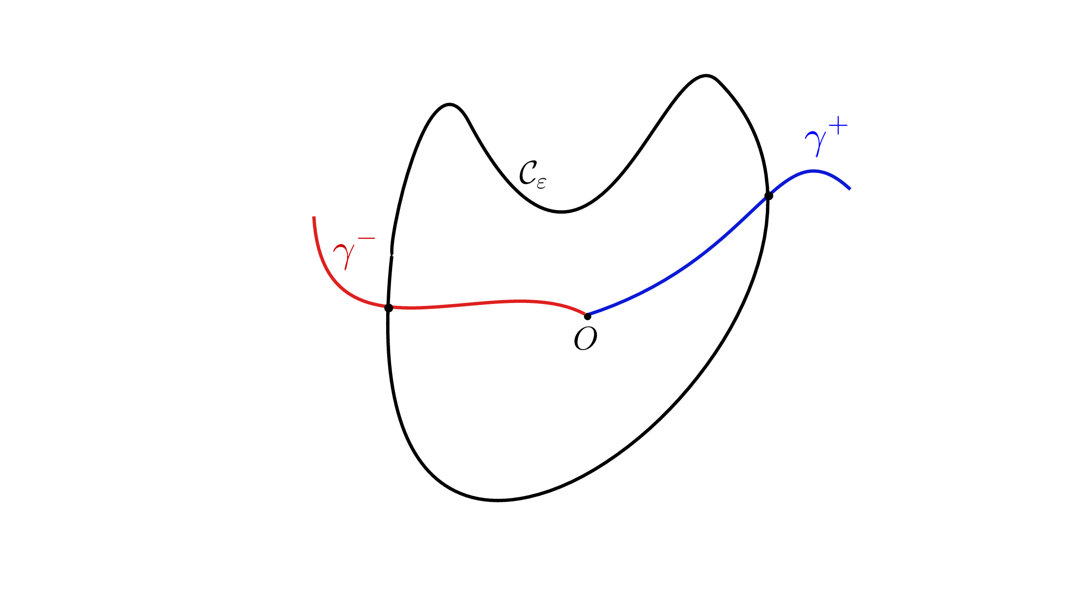 Figure 1
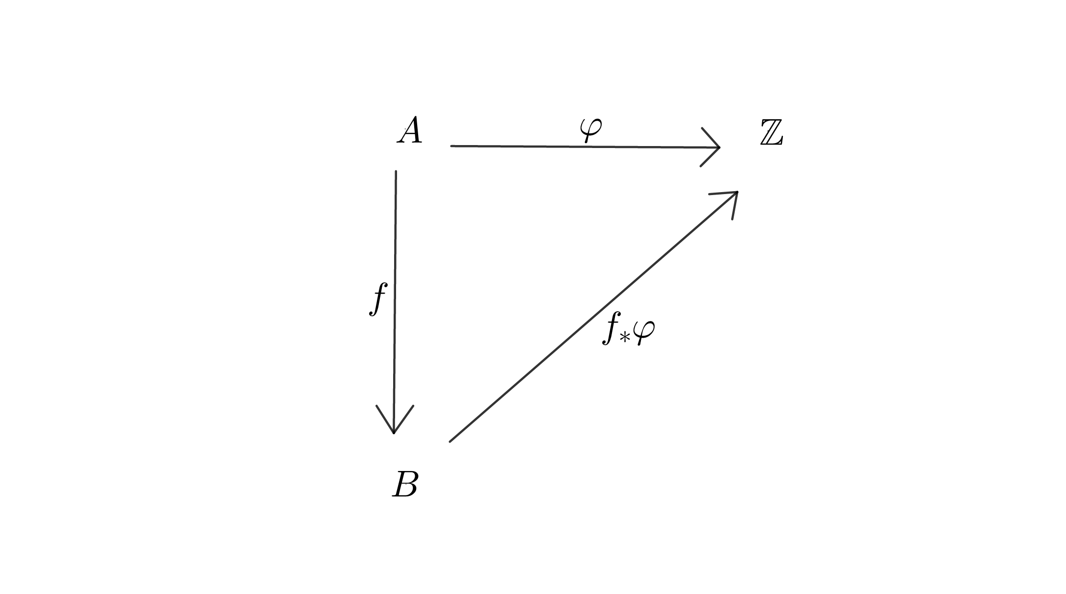 Figure 2
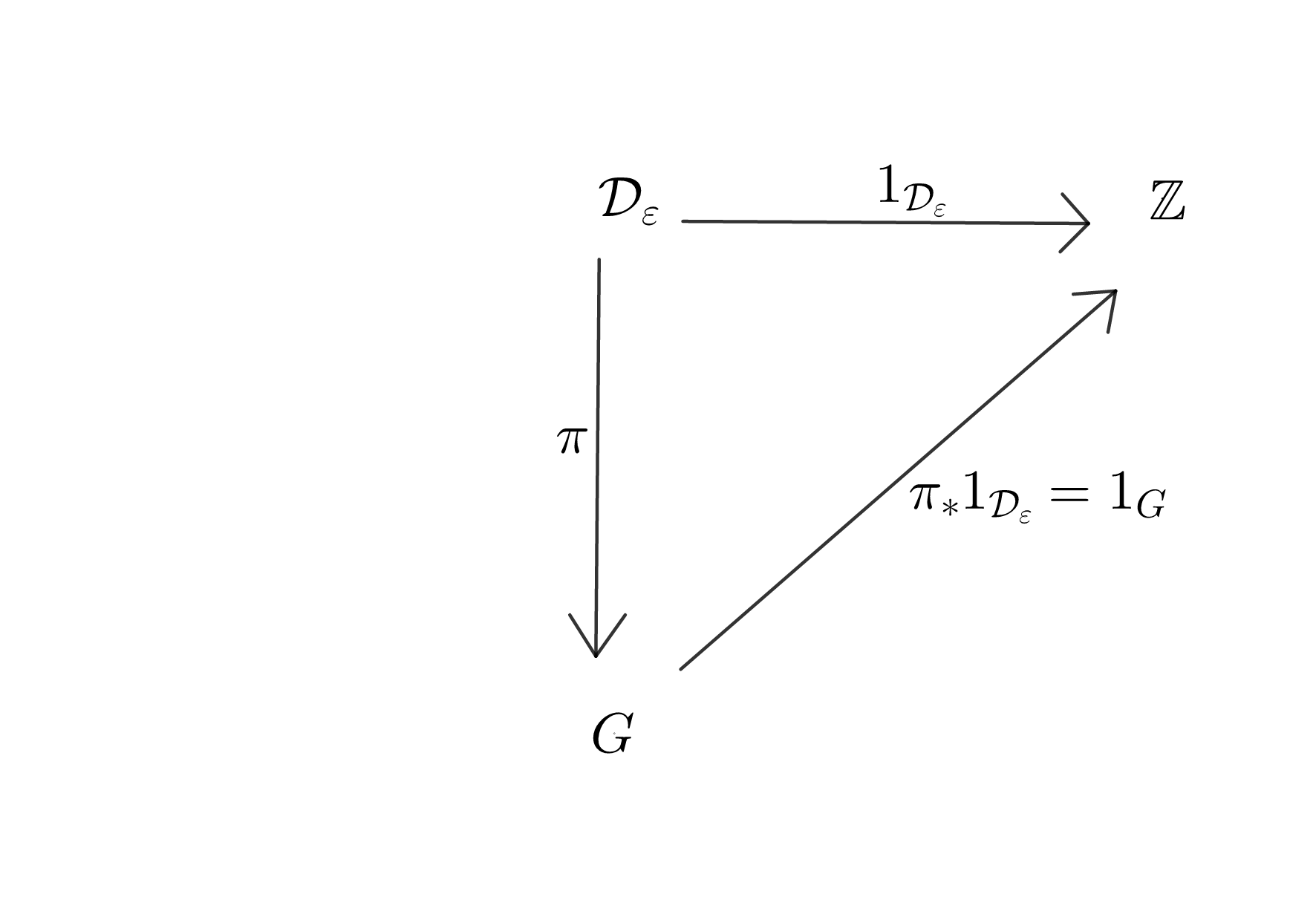 Figure 3
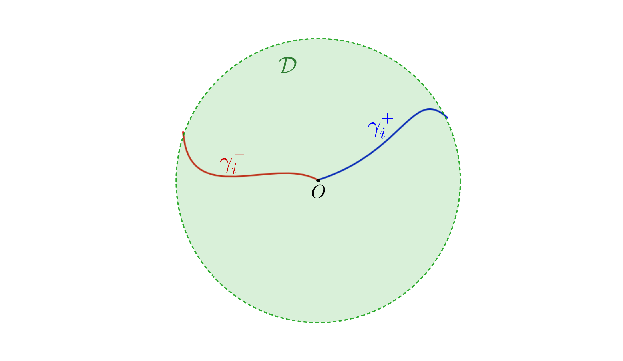 Figure 4
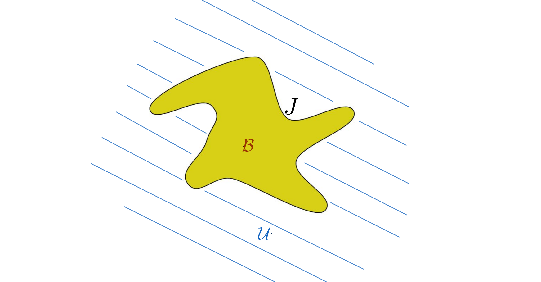 Figure 5
 Figure 6
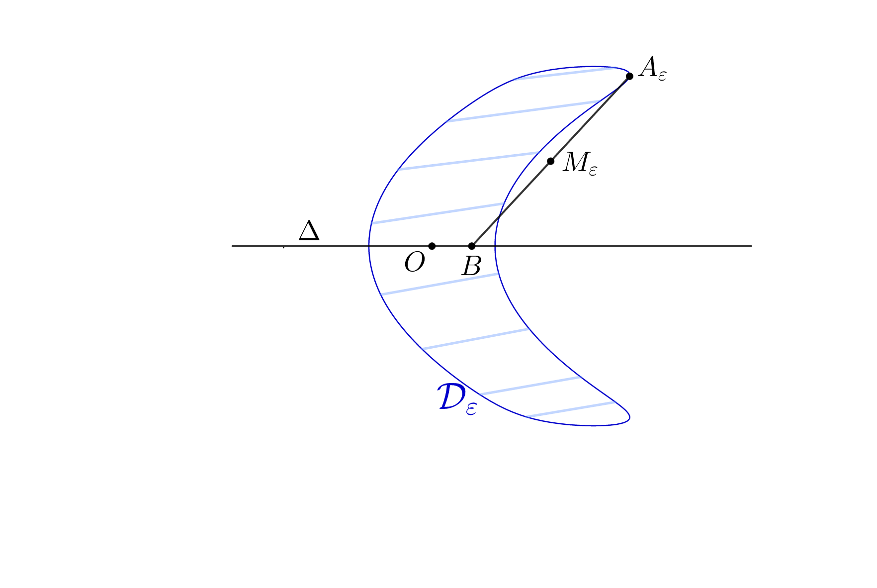 Figure 7
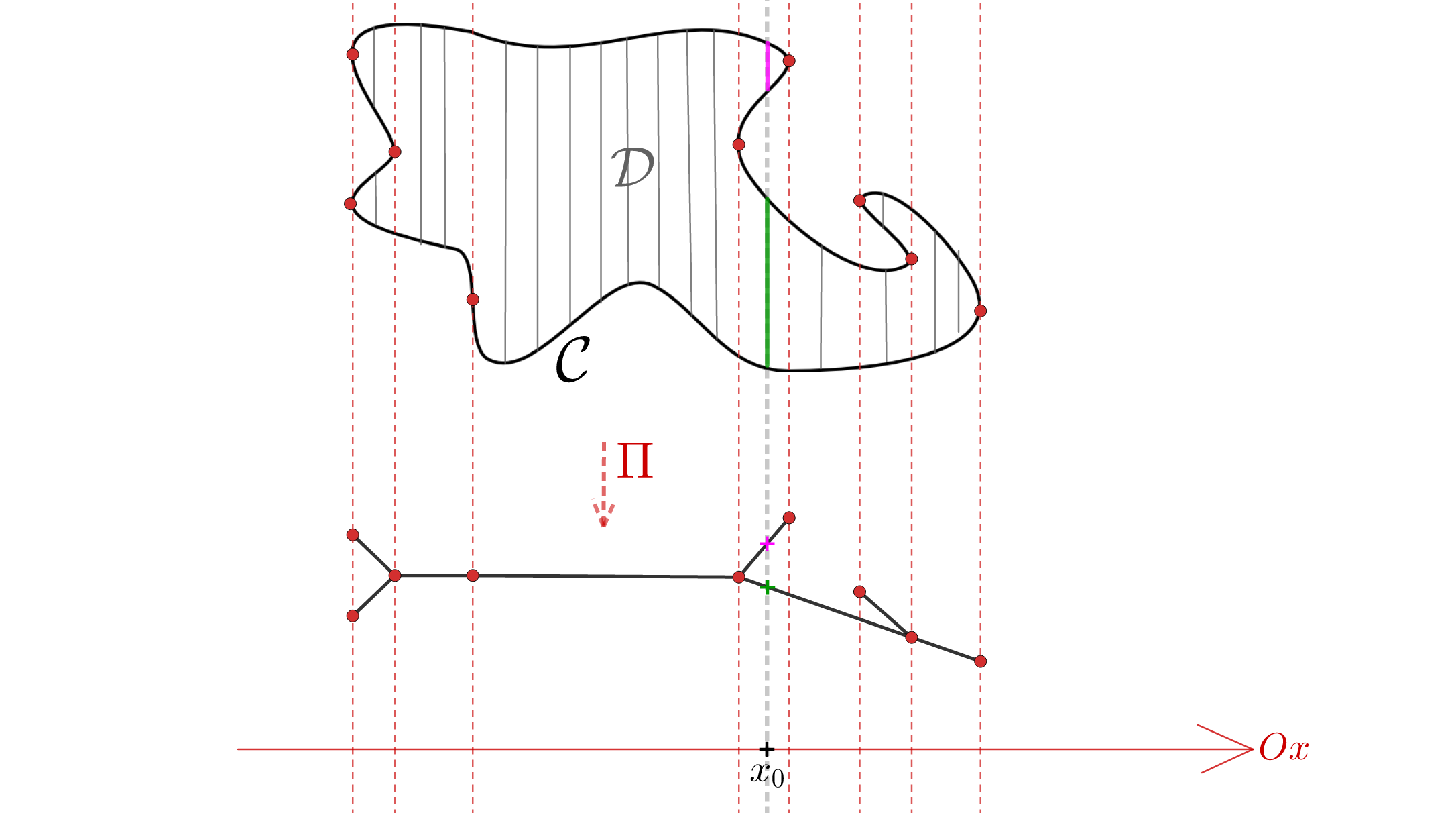 Figure 8
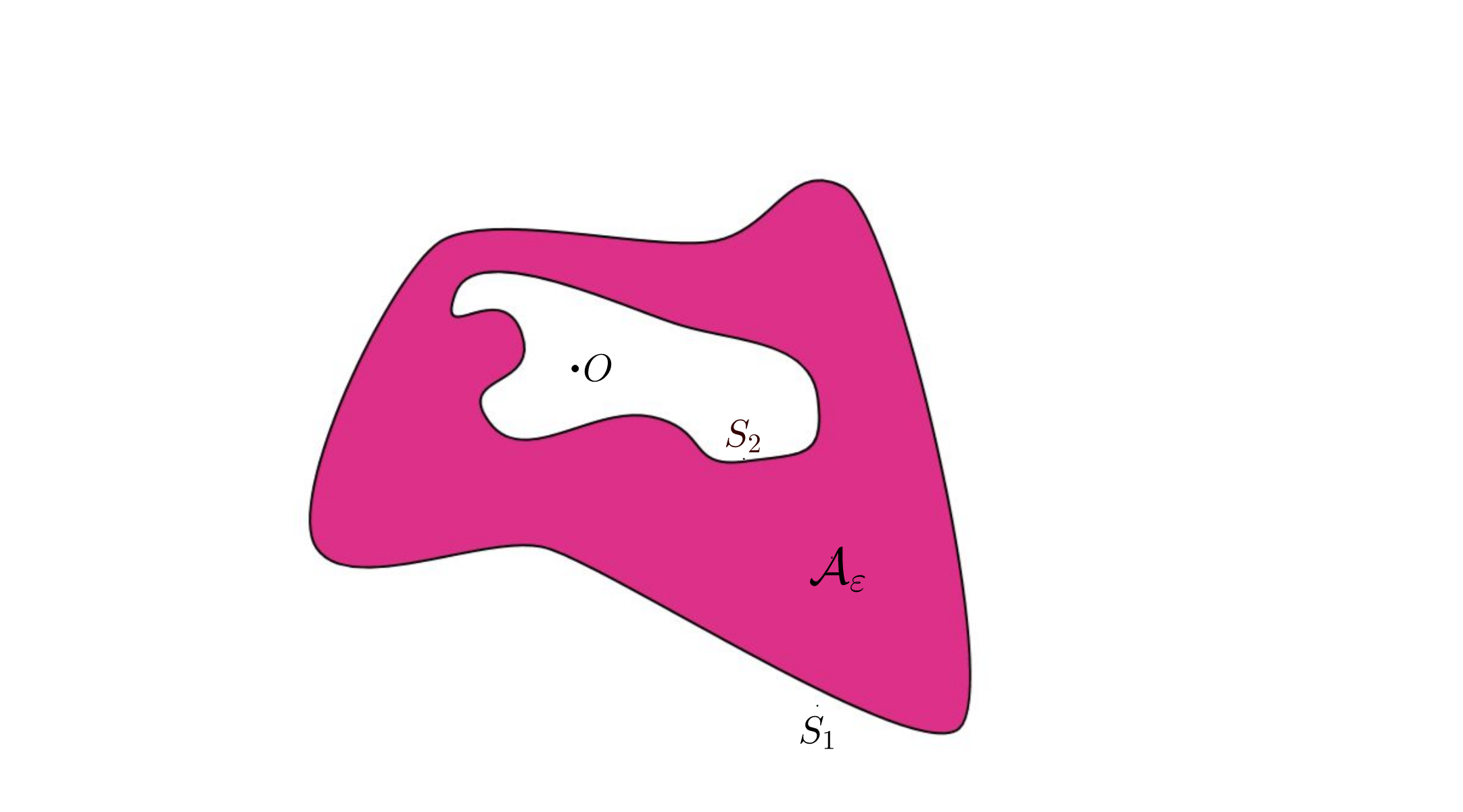 Figure 9
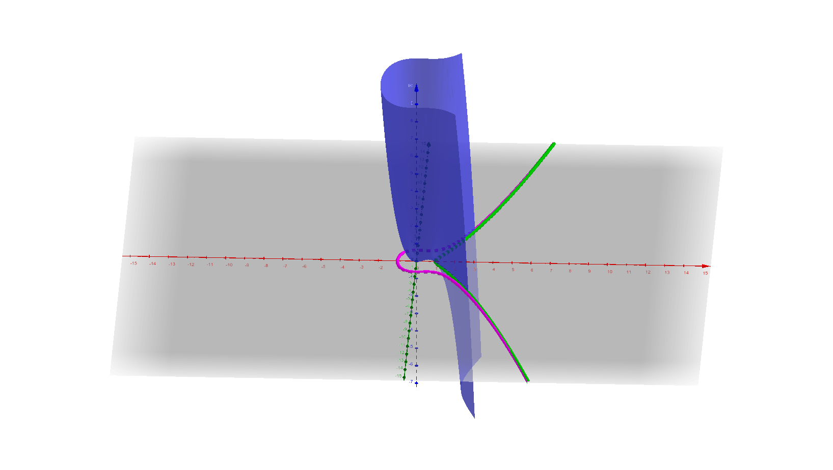 Figure 10
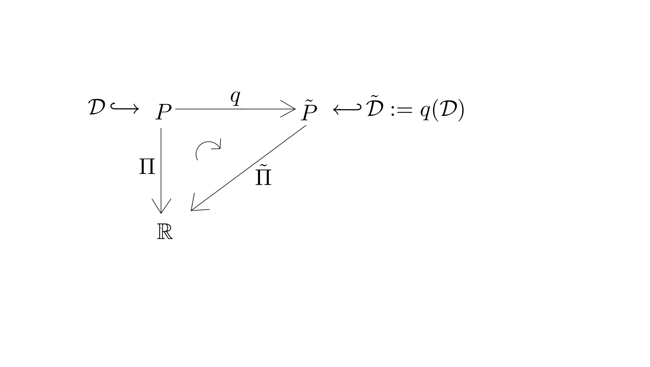 Figure 11
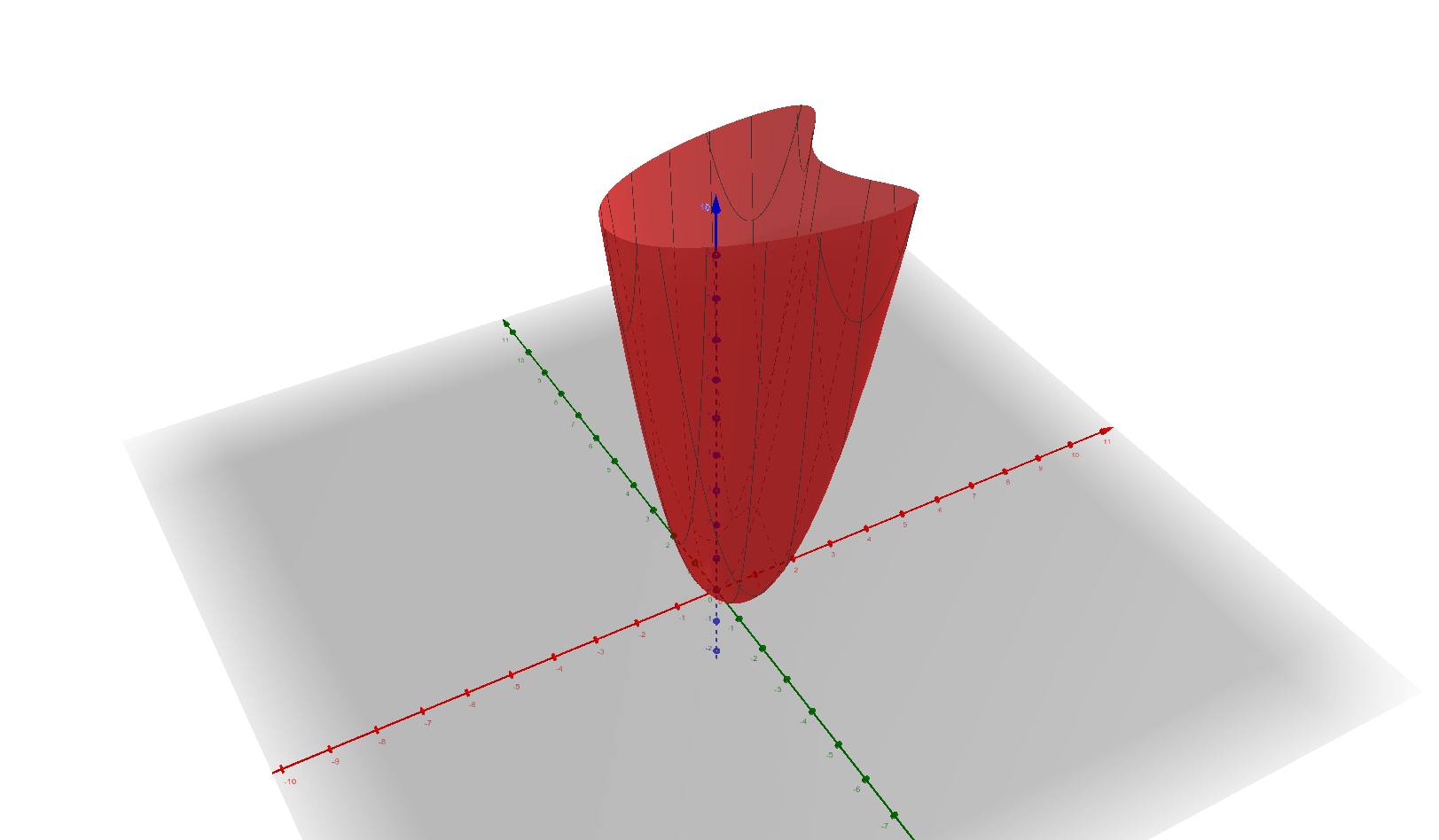 Figure 12
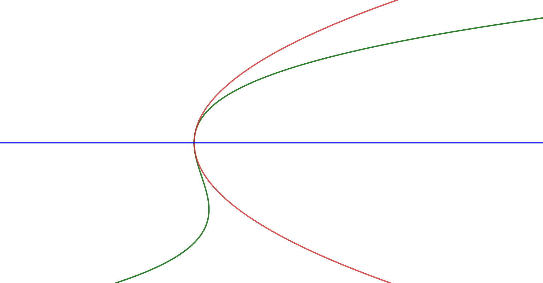 Figure 13
 Figure 14
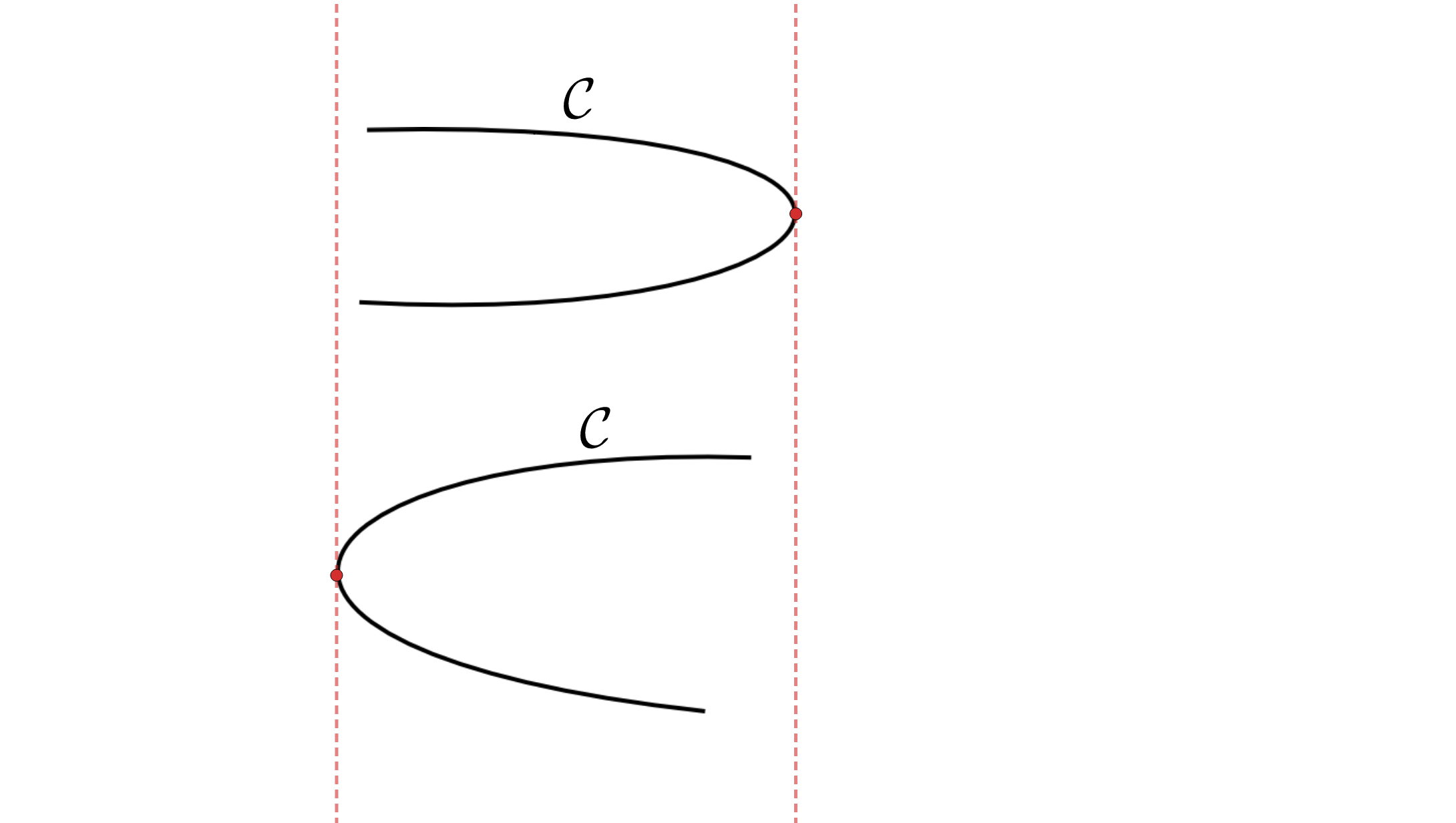 Figure 15
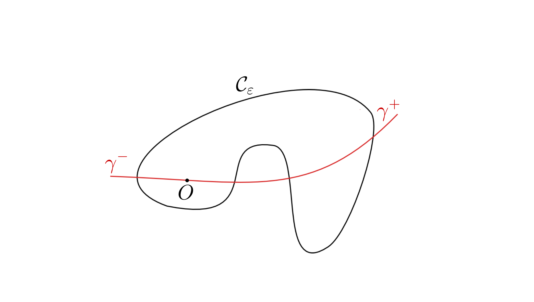 Figure 16
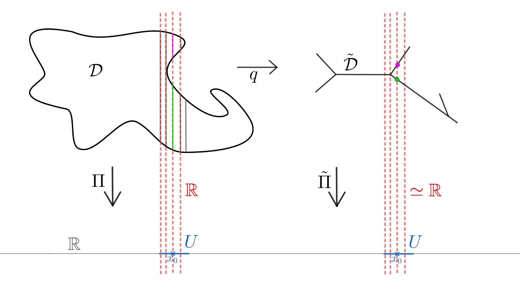 Figure 17
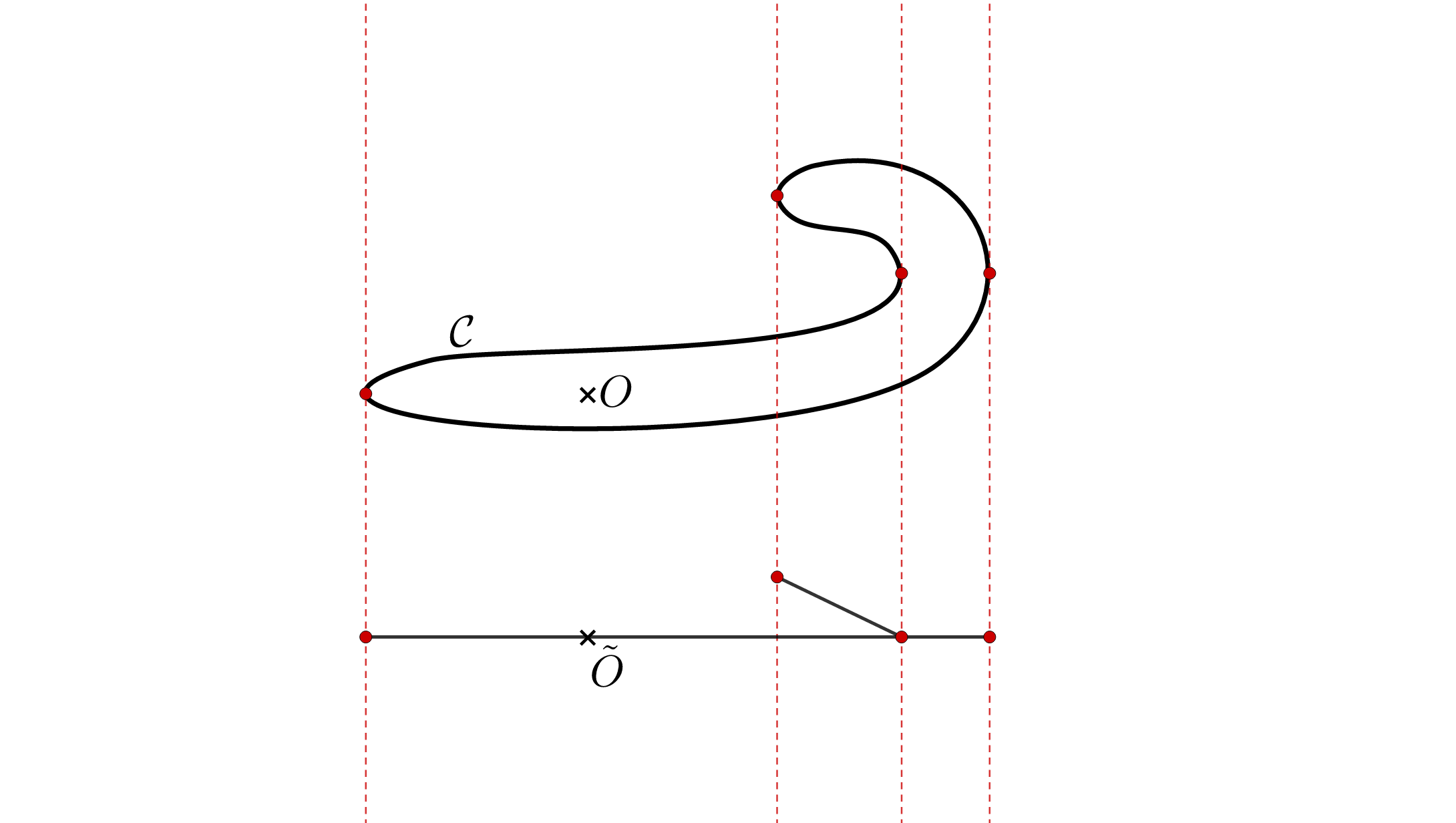 Figure 18
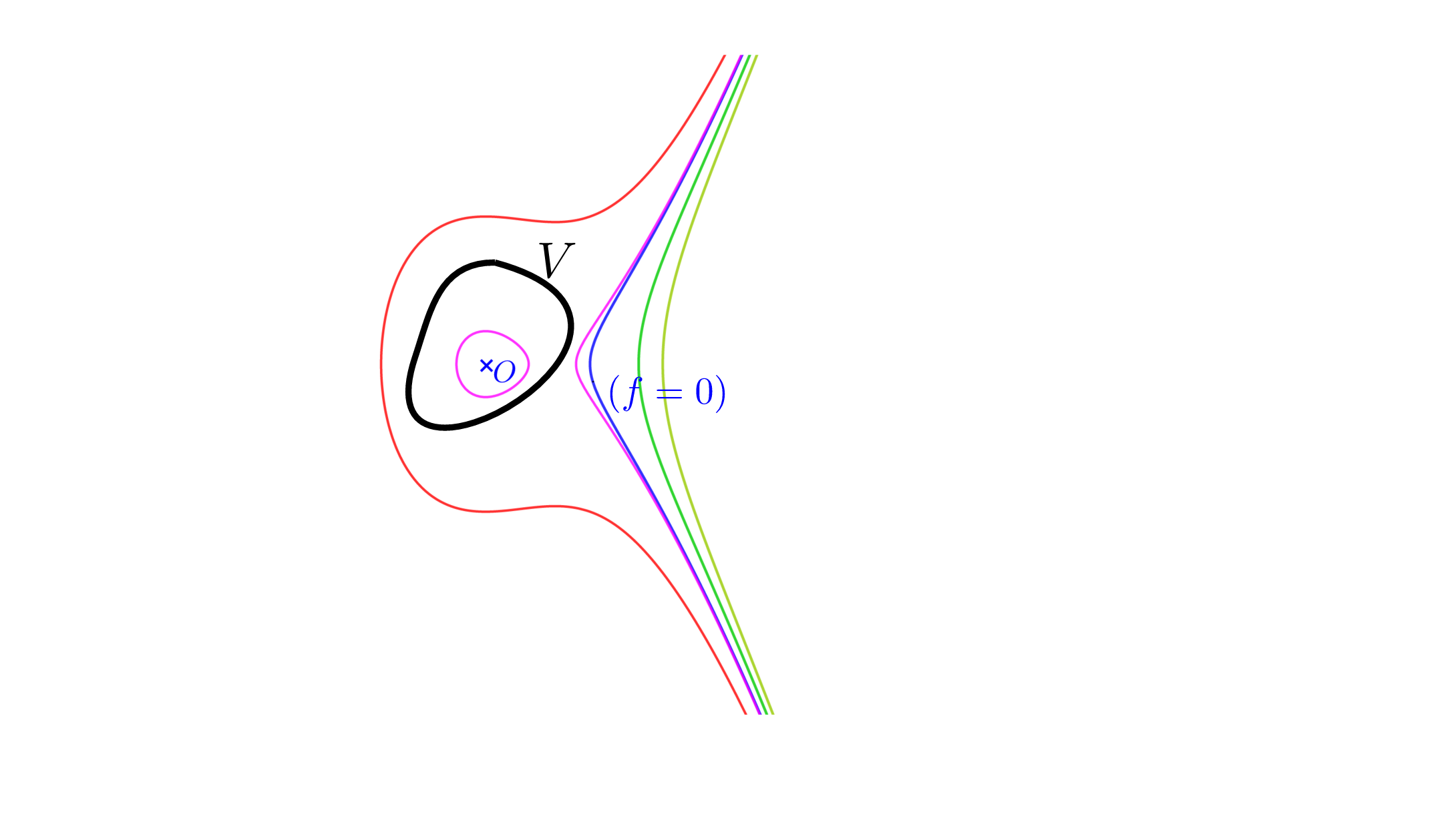 Figure 19
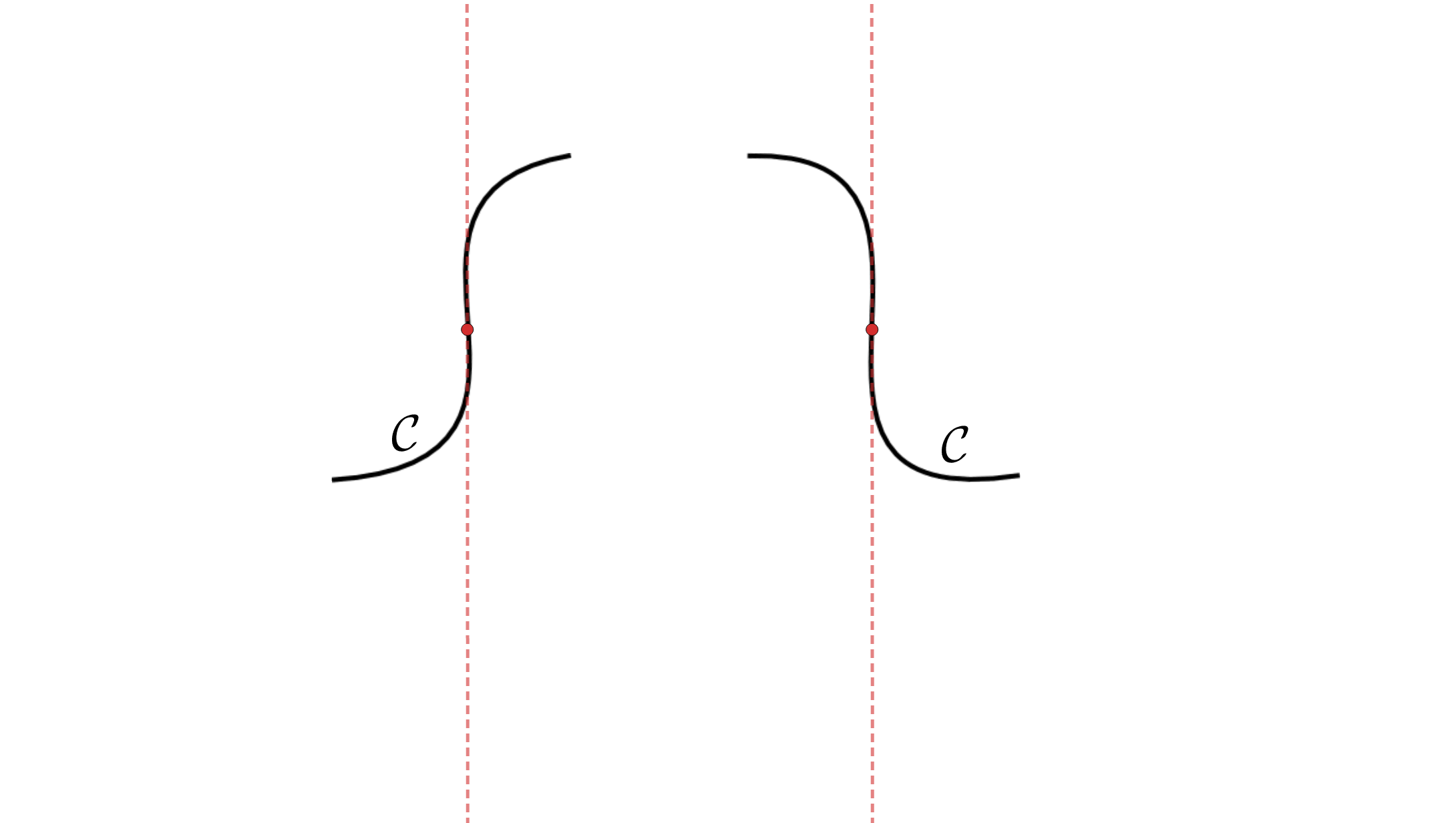 Figure 20
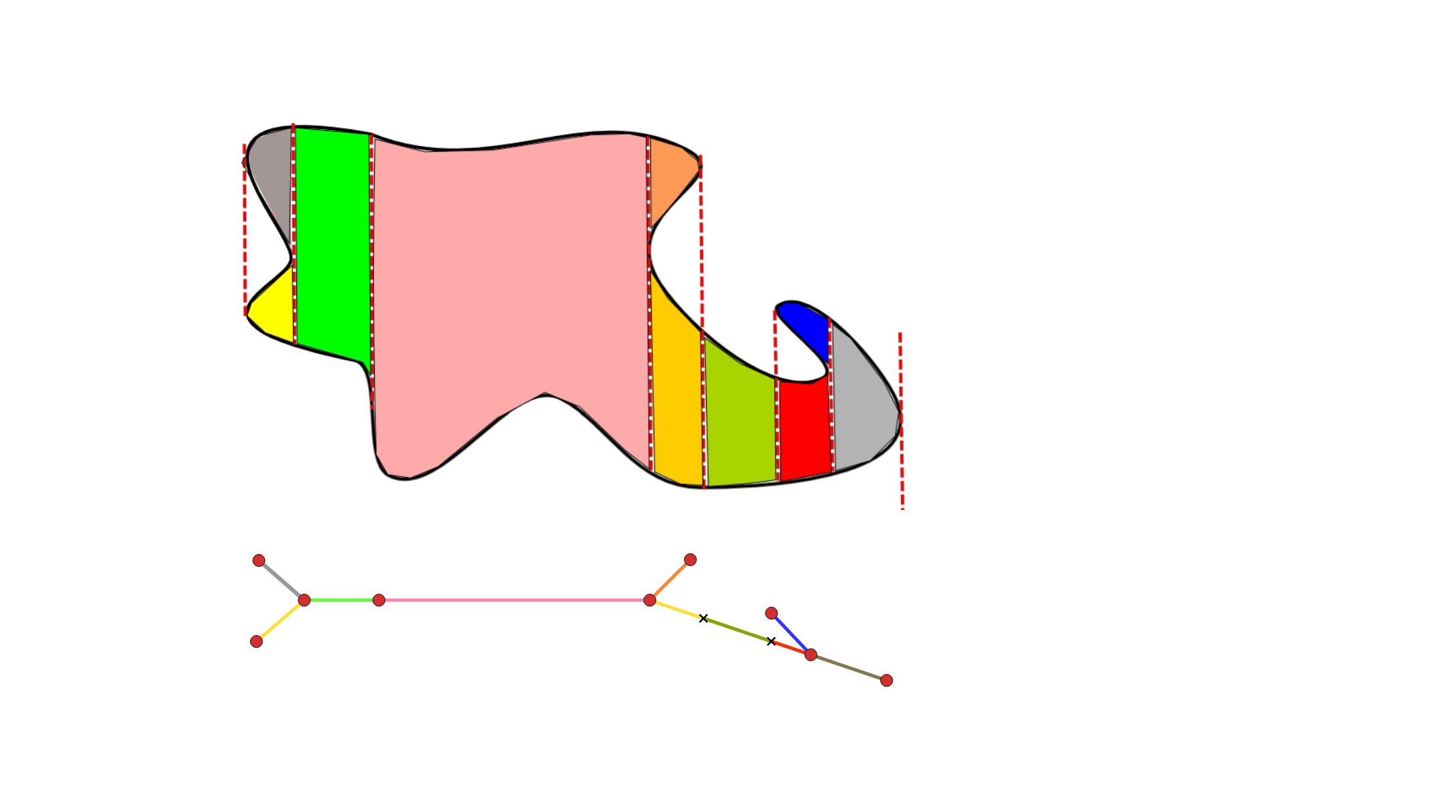 Figure 21
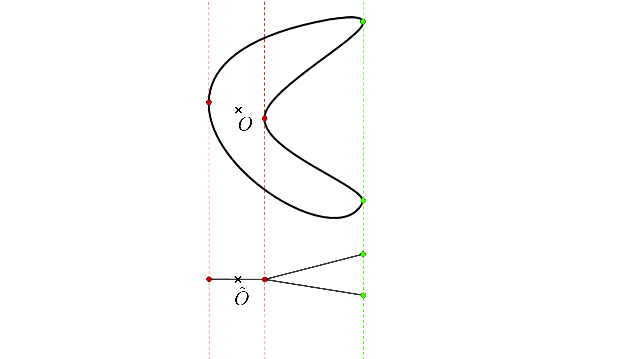 Figure 22
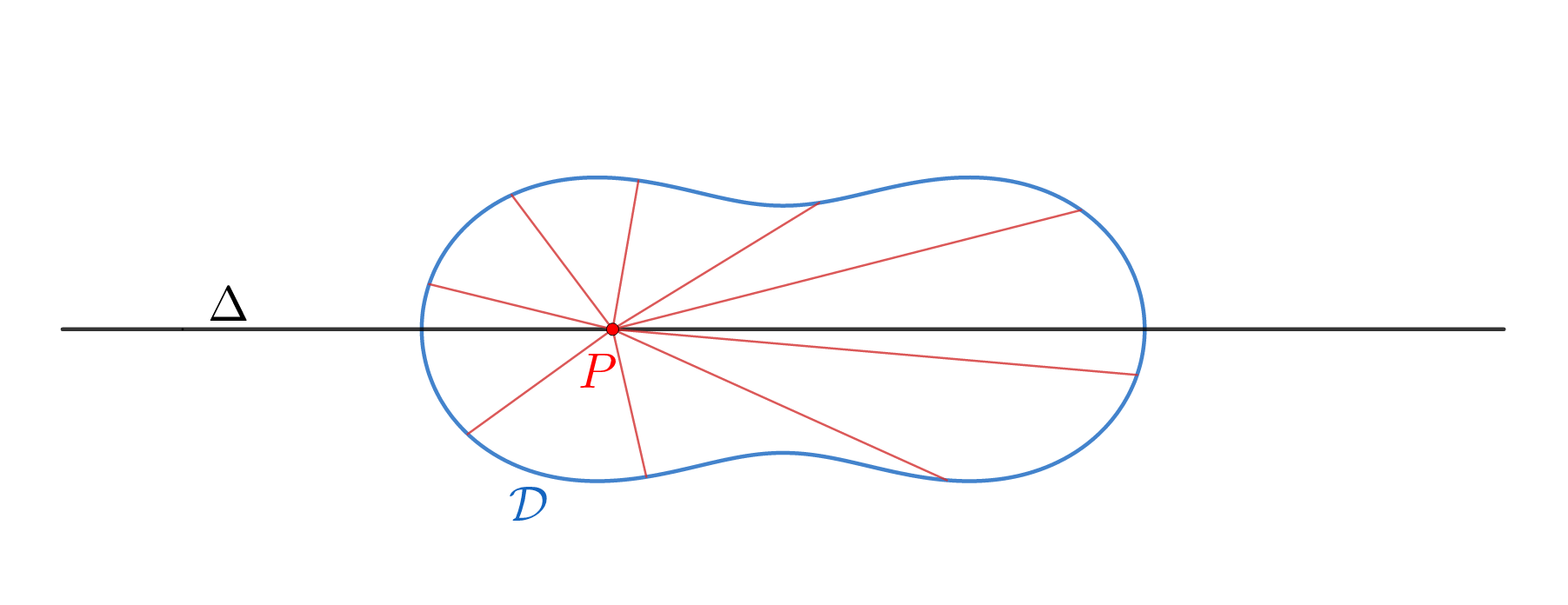 Figure 23
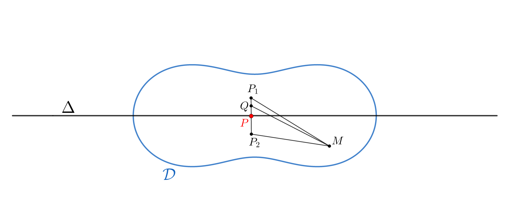 Figure 24
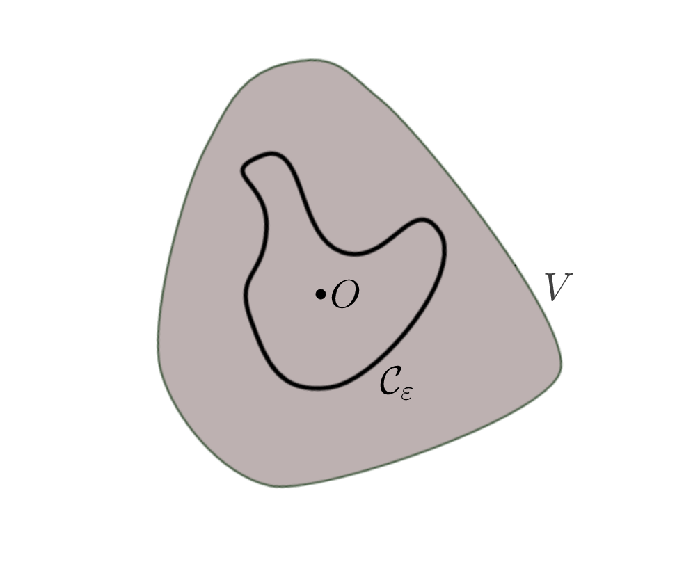 Figure 25
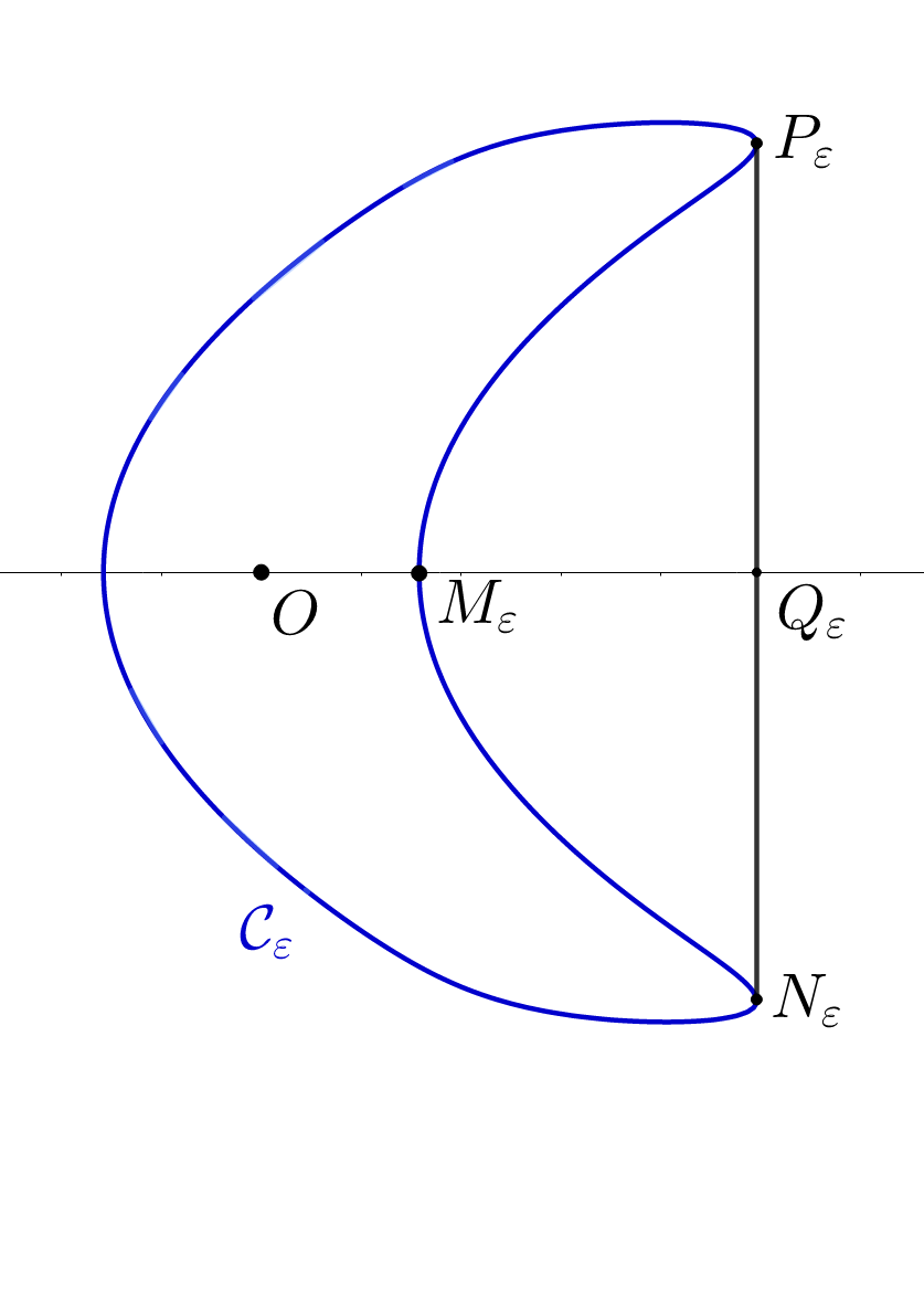 Figure 26
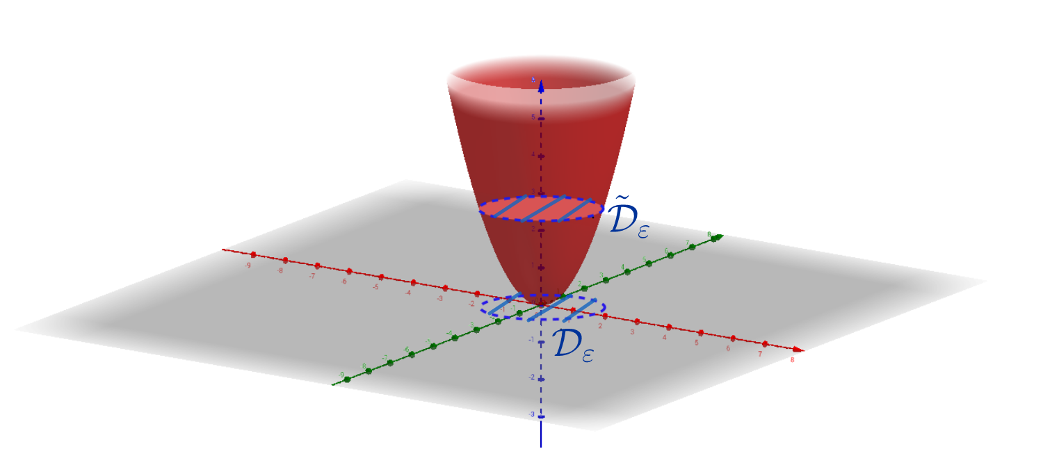 Figure 27
 Figure 28
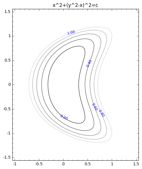 Figure 29
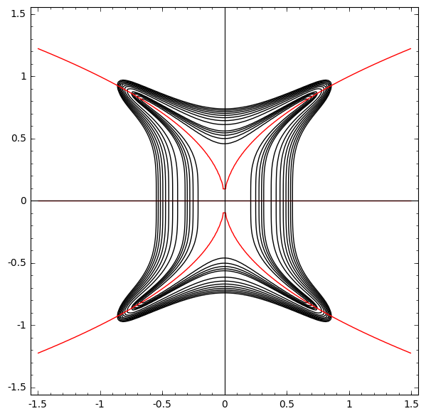 Figure 30
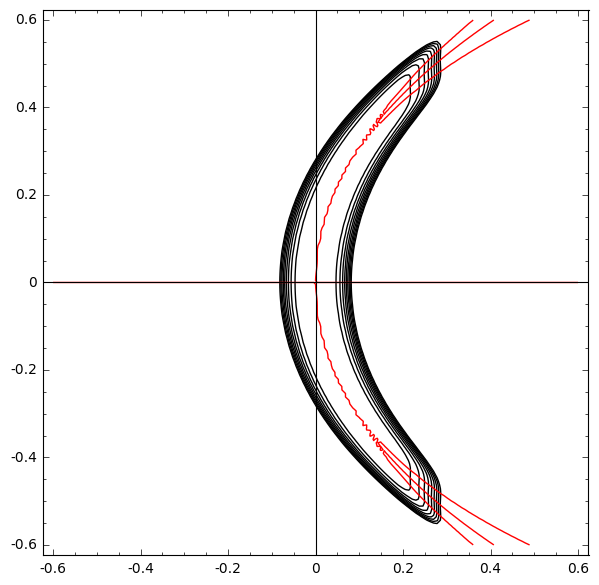 Figure 31
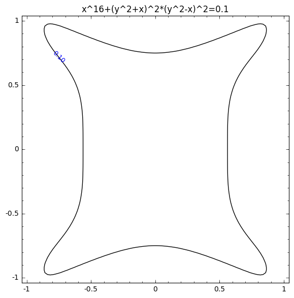 Figure 32
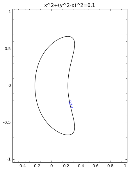 Figure 33
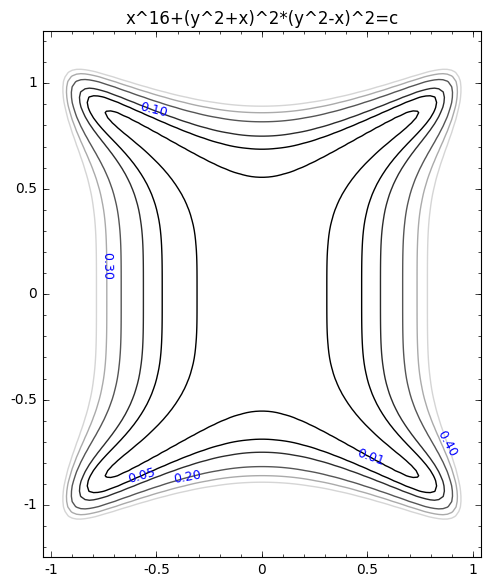 Figure 34
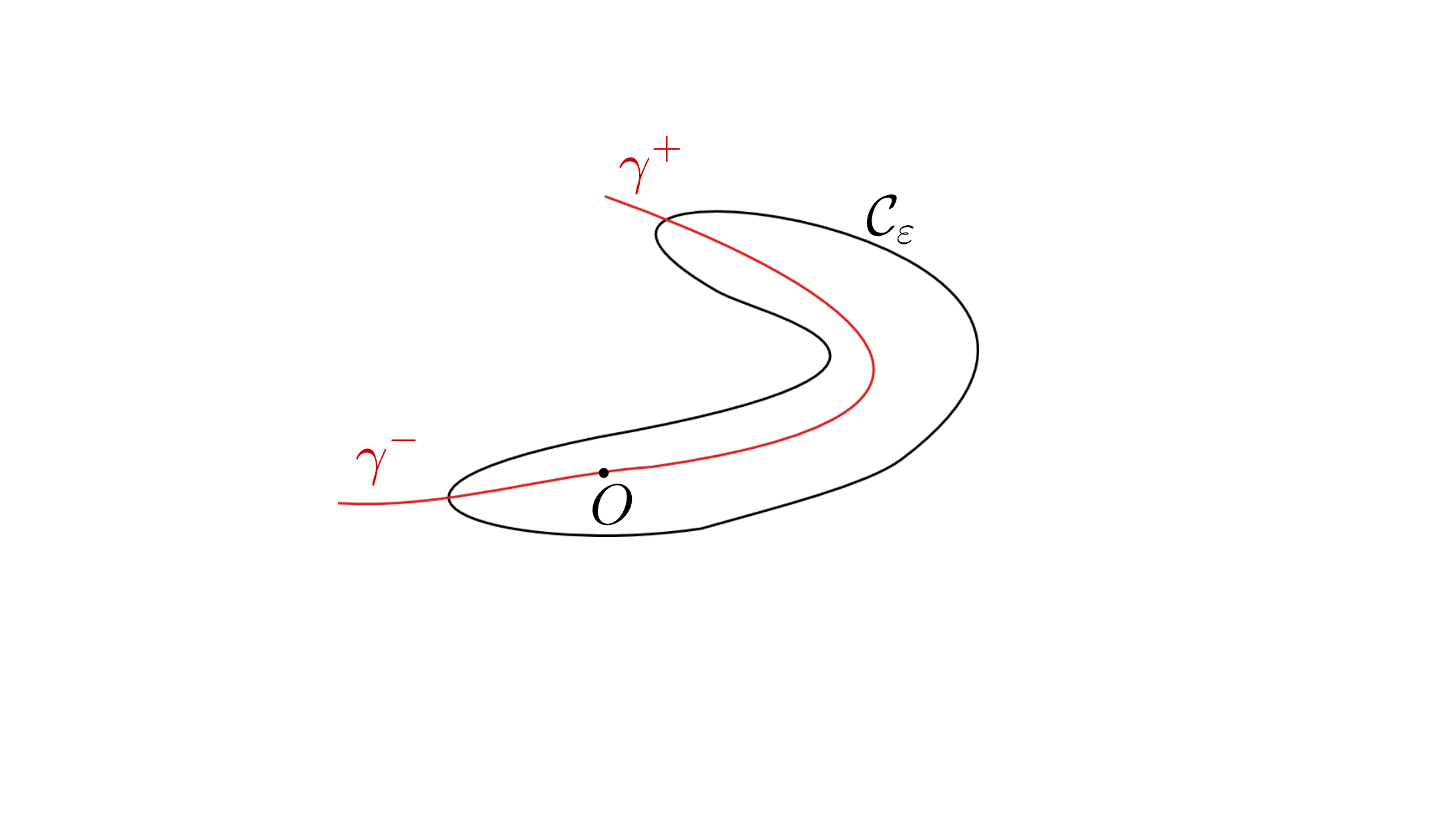 Figure 35
Peer Reviews
No public reviews on file for this paper yet. If you reviewed it on a platform where reviews are public (OpenReview, ICLR, NeurIPS, ICML), you can paste yours below so the community can read it here.
Videos
No videos yet. Explain this paper in a talk, walkthrough, or lecture? Add one.
Taxonomy
TopicsPolynomial and algebraic computation · Advanced Differential Equations and Dynamical Systems · Geometry and complex manifolds
Measuring the local non-convexity of real algebraic curves
Miruna-Ştefana Sorea
Max-Planck-Institut für Mathematik in den Naturwissenschaften, Leipzig, Germany
Key words and phrases:
strict local minimum, Poincaré-Reeb tree, non-convexity, level curve, stabilisation, real algebraic curve, polar curve, star domain, smooth Jordan curve
Abstract
The goal of this paper is to measure the non-convexity of compact and smooth connected components of real algebraic plane curves. We study these curves first in a general setting and then in an asymptotic one. In particular, we consider sufficiently small levels of a real bivariate polynomial in a small enough neighbourhood of a strict local minimum at the origin of the real affine plane. We introduce and describe a new combinatorial object, called the Poincaré-Reeb graph, whose role is to encode the shape of such curves and allow us to quantify their non-convexity. Moreover, we prove that in this setting the Poincaré-Reeb graph is a plane tree and can be used as a tool to study the asymptotic behaviour of level curves near a strict local minimum. Finally, using the real polar curve, we show that locally the shape of the levels stabilises and that no spiralling phenomena occur near the origin.
Introduction
This work is situated at the crossroads between the geometry and topology of singularities and the study of real algebraic plane curves. The origins of this subject date back to the works of Harnack, Klein, and Hilbert ([Har76], [Kle73], [Hil91]). Continuous progress and recent interest on these subjects is shown for instance by Coste, de la Puente, Dutertre, Ghys, Itenberg, Sturmfels, and Viro ([CP01], [Dut16], [Ghy17], [IMR18],[Stu+17], [Vir08]).
Our goal is to measure how far from being convex a given algebraic curve is and what is its behaviour near a strict local minimum. Non-convexity plays an important role in many applications, such as optimisation theory or computational geometry (see for instance [JK17] or [Jut+19]). To this end, we construct and study a new combinatorial object called the Poincaré-Reeb tree, whose role is to encode the shape of a smooth compact connected component of a real algebraic plane curve. In particular, we will use this tool to quantify the non-convexity of the curve. The Poincaré-Reeb tree is adapted from the classical construction introduced by H. Poincaré (see [Poi10, 1904, Fifth supplement, page 221]), which was rediscovered by G. Reeb in 1946 (in [Ree46]). Both used it as a tool in Morse theory. Namely, given a Morse function on a closed manifold, they associated it a graph as a quotient of the manifold by the equivalence relation whose classes are the connected components of the levels of the function. We will perform an analogous construction for a special type of manifold with boundary. We prove that in our setting the Poincaré-Reeb graph is a plane tree, and show several other properties of this tree.
Note that there exist results on graphs encoding the topology of real algebraic plane curves (see, for example, [Che+10] and the references therein). Those graphs are different from our novel Poincaré-Reeb construction.
We will now list the main contributions of this paper.
Measuring the non-convexity via the The Poincaré-Reeb tree. Consider a compact and smooth connected component of a real algebraic curve contained in the plane (see Figure 1). Denote by the disk bounded by . Endow the plane with its canonical orientation and with its foliation by vertical lines. The curve , being a connected component of an algebraic curve, has only finitely many points of vertical tangency. The vertices of the Poincaré-Reeb graph are images of the points of the curve having vertical tangent by the projection , . For if the fibre is not the empty set, then it is a finite union of vertical segments. We define an equivalence relation that lets us contract each of these segments into a point. By the quotient map, the image of the initial disk becomes a one-dimensional connected topological subspace embedded in the real plane. More precisely, it is a connected plane graph. In addition to this construction, we prove the following result:
Theorem 0.1** (see Corollary 4.21).**
The Poincaré-Reeb graph associated to a compact and smooth connected component of a real algebraic plane curve and to a direction of projection is a plane tree whose open edges are transverse to the foliation induced by the function . Its vertices are endowed with a total preorder relation induced by the function .
Note that the main tool used in the proof of Theorem 0.1 is the integration of constructible functions with respect to the Euler characteristic (see [Cos05, Chapter 3, page 22]).
Nested level curves of a real bivariate polynomial near a strict local minimum. Let us consider a polynomial function , such that has a strict local minimum at the origin and . We focus on the so-called real Milnor fibres at the origin of , namely the small enough level curves for sufficiently small We prove that they are smooth Jordan curves (see Lemma 5.3). The simplest example is the circle. Whenever the origin is a Morse strict local minimum, we show that the small enough levels become boundaries of convex topological disks. In the non-Morse case, these curves may fail to be convex, as was shown by a counterexample found by Michel Coste. Let us restrict the study of the Poincaré-Reeb trees to the asymptotic setting, namely let us study the trees associated to small enough level curves of a real bivariate polynomial function, near a strict local minimum at the origin of the plane. We show that the tree stabilises for sufficiently small level curves. We call it the asymptotic Poincaré-Reeb tree. Therefore the shape of the levels stabilises near the strict local minimum (see Figure 2).
We also prove the following result:
Theorem 0.2** (see Theorem 5.31).**
The asymptotic Poincaré-Reeb tree is a rooted tree and the total preorder relation on its vertices, induced by the function , is strictly monotone on each geodesic starting from the root.
The strict monotonicity on the geodesics starting from the root allows us to prove that the small enough level curves have no turning back or spiralling phenomena.
In other words, near a strict local minimum, for sufficiently small there are no level curves like the one in Figure 3.
The present paper is organised as follows. After introducing the necessary notations and hypotheses in Section 1, we show in Section 2 that topological disks bounded by the level curves of in a small enough neighbourhood of a Morse strict local minimum are convex sets (see Theorem 2.3). Section 3 is dedicated to Coste’s counterexample (see Example 3.1) in the non-Morse case and our generalisations. In Section 4 we give the construction of a new combinatorial object, called the Poincaré-Reeb graph, whose role is to measure the non-convexity of a compact smooth connected component of a plane algebraic curve in . Using a Fubini-type theorem and integration with respect to the Euler characteristic, we show that the Poincaré-Reeb graph is in fact a plane tree (see Corollary 4.21). Section 5 focuses on the asymptotic case, where the real polar curve plays a key role. We prove that in a small enough neighbourhood of the origin the Poincaré-Reeb trees become equivalent, starting with a small enough level. In other words, the shape of the levels stabilises near the origin. In addition, the Poincaré-Reeb tree allows us to prove Theorem 5.31. Namely we show that asymptotically there is no spiralling phenomenon near the strict local minimum. This is due to the fact that the induced preorder endowing the set of vertices is strictly monotonous on each geodesic starting from the root of the tree.
Acknowledgements
This paper represents a part of my PhD thesis (see [Sor18]), defended at Paul Painlevé Laboratory, Lille University and financially supported by Labex CEMPI (ANR-11-LABX-0007-01) and by Région Hauts-de-France. I would like to express my gratitude towards my PhD advisors, Arnaud Bodin and Patrick Popescu-Pampu, for their guidance throughout this work. I would like to thank Evelia R. García Barroso and Ilia Itenberg for reviewing my PhD thesis and Étienne Ghys for being the president of the committee.
1. Notations and hypotheses
In this chapter, the expressions “sufficiently small ” or “small enough ” mean: “there exists such that, for any , one has …”. We will often denote this by
We will consider a polynomial function in two variables with . Let us fix a neighbourhood of such that:
-
the point is the only strict local minimum of in ;
-
we have
Definition 1.1**.**
Let us consider a polynomial function that vanishes at the origin , exhibiting a strict local minimum at this point. For , consider the set and denote its connected component that contains the origin by . Denote by
Later on (see Lemma 5.3), we shall prove that for sufficiently small, is diffeomorphic to a circle and that is diffeomorphic to a disk, completely included in .
Example 1.2*.*
The surface of the cubic is shown in Figure 6 (see for instance [Wal78, page 57, Figure 2.2]).
We did not choose yet a sufficiently small neighbourhood of the origin. An illustration of such a neighbourhood that satisfies the hypotheses from Section 1 is shown in Figure 7 below. The zero locus of has two connected components: a point and a curve. We take small enough such that it does not intersect the curve, that is the connected component far from the origin.
Examples of functions as in Section 1 are shown in Figure 8, Figure 10, Figure 12.
For the following classical definition see for instance [Mil68, page 10]:
Definition 1.3**.**
Let with , be a polynomial map.
Let be the maximal rank of , where is the Jacobian matrix of evaluated at
Then the set of singular points (called also critical points) of is by definition
[TABLE]
The image of a singular point under is called a singular value of .
A point is called regular of if it is not singular.
Example 1.4*.*
Let be a polynomial function. Then by Definition 1.3, the set of singular points of is
For more examples, see for instance [PP18] or [Wal78, page 57].
2. Morse extrema and convex level sets
The classical well-known statement that follows is meant to present equivalent characterisations of convex functions (see, for instance, [Rek+83, pages 640-650]).
Theorem 2.1**.**
Let us consider a convex set and a function . The following properties are equivalent:
(1) for any two points , , for any we have
[TABLE]
(2) the set is convex;
(3) the Hessian matrix of , denoted by , is everywhere positive definite or positive semidefinite.
Definition 2.2**.**
A function is convex if verifies one of the properties from Theorem 2.1.
Theorem 2.3**.**
Let be a polynomial function of the form where and is a polynomial function of degree of each monomial at least . Then for a sufficiently small , is a convex set in a small enough neighbourhood of the origin.
Proof.
Note that we are situated in a small enough neighbourhood of the origin. We have , , for any in a small enough neighbourhood of . Thus the Hessian matrix is positive definite and we conclude that is a convex function, since we are in dimension and by Sylvester criterion if a symmetric matrix has all diagonal elements and all the leading principal determinants positive, then the matrix is a positive definite matrix (see [Gil91, page 45], or [Rek+83]). Recall the fact that positive definite forms form an open set in the space of all forms. Since the function is , its Hessian form varies continuously.
Therefore, the epigraph of restricted to a convex domain is a convex set. Let us consider sufficiently small. Since we obtain that is a convex set, since it is the intersection of two convex sets. Thus, the projection of on the plane is also convex, in fact it is equal to .
Let us sketch a second proof. Since for any in a small enough neighbourhood of , the Hessian curve of given by , is empty. Thus (see [Wal04, page 71]) for a sufficiently small the level curve has no inflexion points, hence it is convex.
∎
Example 2.4*.*
The circular paraboloid (see in Figure 8 below): are circles.
3. Non-convex level sets
The starting point of this research is the following question:
Question* (E. Giroux to P. Popescu-Pampu, 2004).*
Are the small enough level curves of near strict local minima always boundaries of convex disks (even for non-Morse singularities)?
Answer: The answer to this question is negative, as the following counterexample by M. Coste shows.
Example 3.1*.*
Let us study the counterexample found by M. Coste:
[TABLE]
See Figure 9(b) for the family of its level sets. Figure 10 illustrates the graph of and Figure 9(a) a single level
The idea used by M. Coste was that instead of taking the sum of squares of functions defining transverse curves like in (i.e. the lines defined by and are transverse), to take the sum of squares of and , which define two curves that are tangent at the origin.
Note that the function was also mentioned in [JK11], [Bol80].
Proposition 3.2**.**
The topological disks from Example 3.1 are never convex for .
Proof.
Indeed, if we denote by , by and by , then we get , , , and , (see Figure 11).
Denote by the midpoint of . Then . Since and there is no other point to the right of , we conclude that Hence there exist the points and such that the segment is not included in In conclusion, we proved that there exists at least a point outside the disk on the segment . ∎
3.1. Generalisations
In the sequel we give some new examples of functions with a strict local minimum at the origin , whose level sets are all boundaries of non-convex disks for a sufficiently small .
The shape of these level curves stabilises for sufficiently small , as we shall prove in this paper.
Example 3.3*.*
Let us take the following polynomial:
[TABLE]
For a family of level curves of , see Figure 12.
Example 3.4*.*
Let us consider the following polynomial:
[TABLE]
The shape of its level curves is sketched in Figure 13.
3.2. Star domains
The following definition is well-known:
Definition 3.5**.**
[AB06, page 168] A set in the Euclidean space is called a star domain with respect to if for all the line segment from to is in .
Proposition 3.6**.**
The polynomial function
[TABLE]
for , has the following properties: is a strict local minimum and for sufficiently small , the set is not a star domain with respect to any point .
Before the proof, let us first present the following Lemma:
Lemma 3.7**.**
If a set is a star domain with respect to a point and if admits a symmetry axis, say (see Figure 14), then there exists a point such that is a star domain with respect to .
Proof.
By hypothesis, the given set is a star domain with respect to a point. Denote this point by . If , there is nothing to prove. Let us consider , as pictured in Figure 15.
By hypothesis, is a symmetry axis for Let us denote by the symmetric of with respect to Denote by the midpoint of the segment . Hence, and by symmetry, is a star domain also with respect to Let us now prove that is a star domain with respect to any point hence is a star domain with respect to the point .
Let . Since is a star domain with respect to both and we have that , and are included in . Thus, both the triangle and its interior are included in since the interior is the union of , for all . In particular, for any point we obtain Namely, is a star domain with respect to any point In conclusion, is a star domain with respect to ∎
In the following let us present the proof of Proposition 3.6.
Proof.
By Lemma 3.7, it is sufficient to prove that is not a star domain with respect to any point on such that , because the line is a symmetry axis for
Consider the point see Figure 16. Then the midpoint of the segment (see Figure 16 below) is the point
[TABLE]
We will prove that
Since we have For sufficiently small , we have sufficiently small, thus Hence
We have .
There are two cases to consider.
First, if , then we have for a sufficiently small
Secondly, if then Since and we obtain Thus, for a sufficiently small and for
In both cases, we get hence and thus the segment is not included in even though In other words, is not a star domain with respect to any ∎
4. The Poincaré-Reeb tree
4.1. The Poincaré-Reeb construction
The main purpose of this section is to introduce a new combinatorial object that measures the non-convexity of a smooth and compact connected component of a real algebraic curve in . We will define the Poincaré-Reeb graph, associated to the given curve and to a direction of projection . It is adapted from the classical construction introduced by H. Poincaré (see [Poi10, 1904, Fifth supplement, page 221]), which was rediscovered by G. Reeb (in [Ree46]). Both used it as a tool in Morse theory (see [Mat02]). Namely, given a Morse function on a closed manifold, they associated it a graph as a quotient of the manifold by the equivalence relation whose classes are the connected components of the levels of the function. We will perform an analogous construction for a special type of manifold with boundary, namely for a topological disk bounded by a smooth and compact connected component of a real algebraic curve. We prove that in our setting the Poincaré-Reeb graph is a plane tree.
Let us consider a smooth and compact connected component of a real algebraic curve in , denoted by . Let denote the topological disk bounded by (see Figure 17 below). Moreover, let us define the projection
Definition 4.1**.**
For each , is a finite union of connected vertical segments. Let us define the equivalence relation as follows: if and are two points in the real plane then if and only if they belong to the same vertical connected component of the fibre .
Given the above equivalence relation, let us consider the canonical quotient map
[TABLE]
Denote by and by The coordinates in are with
The function descends to the quotient in a function The function is continuous, since is continuous.
We obtain the following commutative diagram (see Figure 18):
Our next aim is to prove that is homeomorphic to . First we show that endowed with the function is a fibre bundle, i.e. that satisfies a local triviality. We will prove that it is locally a cartesian product of two sub-spaces. Furthermore, we shall prove that the local trivialisation of the fibre bundle implies that is a trivial fibre bundle, i.e. it is not just locally a product of two spaces, but globally.
Proposition 4.2**.**
The topological space endowed with the function is a fibre bundle.
Proof.
By the definition of the fibre bundle (see for instance [Frè13, page 51]), what we need to prove is that there exists a local trivialisation of . Let us consider a point in the base space, that is the -axis. Take an open neighbourhood of called We want to show that the set is homeomorphic to here by R we mean a space that is homeomorphic to the real line To this end, we have the following two arguments:
-
If on a vertical line we contract a finite number of segments into points (by the quotient map described above), we obtain a topological space that is homeomorphic to Denote this space by
-
The set is a finite union of intervals (some of them empty intervals), whose extremities depend continuously on (see Figure 19), except when is a critical point.
Hence we have the local triviality: is homeomorphic to Thus the image of the plane , by the quotient map , is a fibre bundle.
∎
Proposition 4.3**.**
The topological space endowed with the function is a trivial fibre bundle.
Proof.
The base space of the fibre bundle is the -axis, namely , and is contractible to a point. Thus we conclude that is a trivial fibre bundle, since by [Osb82, Proposition 3.5, page 75] a fibre bundle over a base space that is contractible to a point is trivial. To be more precise, we have homeomorphic to ∎
Corollary 4.4**.**
The topological subspace is embedded in a real plane.
Theorem 4.5**.**
The topological subspace is connected.
Proof.
The image of a connected space by a continuous function is connected. Since , the topological disk is connected and the quotient map is continuous, the proof is complete. ∎
Theorem 4.6**.**
The topological subspace is a one-dimensional subspace of . In each of the regular points of , we have transverse to the foliation of the plane by vertical lines, induced by .
Proof.
Since the curve is a connected component of a real algebraic curve, that is, it is an analytic curve, it has finitely many points of vertical tangency. In other words, there are finitely many critical levels of the projection . Locally near a critical point, one may have a tangency point of even order (see Figure 20(a)) or of odd order (see Figure 20(b)):
Between any two critical levels, we have only what we call “bands” of the initial disk . See, for a better comprehension, Figure 21 below. After taking the quotient, each band contracts into an arc of dimension one, transverse to the vertical foliation of the real plane . Therefore, the topological space is a graph, being a finite union of transverse arcs.
Definition 4.7**.**
[Vic89, pages 13-14] A preorder on a set is a binary relation that is reflexive and transitive.
Definition 4.8**.**
Given the projection let us consider the image of the topological disk bounded by the smooth and compact connected component of a real algebraic curve , where the quotient map introduced before. The image endowed with special vertices, namely the finitely many points corresponding to the critical points of on is called the Poincaré-Reeb graph associated to the curve and to . Endow the real plane with the trivial fibre bundle , then endow the vertices of the graph with the induced preorder.
∎
In conclusion, the Poincaré-Reeb construction that we introduce in this paper gives us a plane connected graph, embedded in a surface that is homeomorphic to . We will prove in the next section that it is in fact a tree.
4.2. Constructible functions and a Fubini type theorem
In this section we will recall the integration of constructible functions with respect to the Euler characteristic and a Fubini-type theorem for it. Then we will apply it to the proof of Proposition 4.20.
We will first introduce the necessary tools: constructible functions. We shall follow the definitions and results from [Cos05, Chapter 3, pages 21-22]. For more details, the reader should refer to [Wal04, page 162]. Constructible functions have applications in the study of the topology of singular real algebraic sets (see for instance [Dut16]). The main tool is the integration against the Euler characteristic, which was first described in Viro’s paper [Vir88].
Definition 4.9**.**
[Cos02, page 25] A basic semialgebraic set is a subset of satisfying a finite number of polynomial equations and inequalities with real coefficients.
Example 4.10*.*
All algebraic sets are basic semialgebraic.
Unions of finitely many points and open intervals in are basic semialgebraic sets.
Definition 4.11**.**
[Cos02, page 29] Let us consider two basic semialgebraic sets and . We say that a continuous map is a semialgebraic map if its graph is a semialgebraic subset of .
Definition 4.12**.**
[Cos05, Chapter 3, page 21] A constructible function on a semialgebraic set is a function which takes finitely many values and such that, for every , is a semialgebraic subset of .
Remark 4.13*.*
[Wal04, page 162] Each constructible function is an integer linear combination of characteristic functions of constructible sets , i.e. of semialgebraic subsets of :
[TABLE]
where and is the characteristic function of .
Definition 4.14**.**
[Cos05, Chapter 3, page 22] Let be a constructible function on a semialgebraic set . The integral of with respect to the Euler characteristic is by definition:
[TABLE]
where denotes the Euler characteristic.
Definition 4.15**.**
[Cos05, Chapter 3, page 22] Let us consider a continuous semialgebraic map and let be a constructible function on . The pushforward of along (see Figure 22) is the function ,
[TABLE]
Remark 4.16*.*
If we apply the definition of push-forward to the application from a set towards a point, we obtain the function that associates at this point the integral with respect to the Euler characteristic of the starting function on .
Remark 4.17*.*
The diagram from Figure 22 is not commutative. If, for example, , , where are points in , a semialgebraic map such that and a constructible function on such that , , then by definition we compute Thus while . Therefore
Remark 4.18*.*
The following proofs can be extended to semianalytic sets, with the more general hypothesis that is analytic.
Theorem 4.19**.**
[Cos05, Chapter 3, page 22]** Fubini Type Theorem: Let be a semialgebraic map and a constructible function on . Then
[TABLE]
We are ready now to prove the main result of this section, namely Proposition 4.20.
Proposition 4.20**.**
The Poincaré-Reeb graph of a topological disk bounded by a smooth and compact connected component of a real algebraic curve in is a tree.
Proof.
In Definition 4.15 let us replace with the disk with the graph obtained after the Poincaré-Reeb contraction , the function with the Poincaré-Reeb contraction and with the characteristic function , as in Figure 23:
In other words, we apply the Fubini Type Theorem 4.19 for the pushforward of the constructible function .
Now for , we obtain:
[TABLE]
since is a connected component of the fibre, i.e. a segment. Thus
[TABLE]
By Theorem 4.19, we have now
[TABLE]
Since we obtain:
[TABLE]
Therefore, Since is a disk, we have In Section 4 we proved that is a connected graph, thus the Betti number . We have Since we proved that its Euler characteristic is we get that the Betti number . Thus we conclude that has no cycles, hence is a tree.
∎
Corollary 4.21**.**
The Poincaré-Reeb graph associated to a compact and smooth connected component of a real algebraic plane curve and to a direction of projection is a plane tree whose open edges are transverse to the foliation induced by the function . Its vertices are endowed with a total preorder relation induced by the function .
Definition 4.22**.**
A transversal tree is a finite tree embedded in a real oriented plane endowed with a trivialisable fibre bundle , such that each one of its edges is transversal to the fibres of .
Two transversal trees and are considered to be equivalent if there exists an orientation preserving homeomorphism sending one pair into the other one and one fibre bundle into the other one (in the sense that there exists an orientation-preserving homeomorphism such that ).
5. Asymptotic behaviour of curves near a strict local minimum
Let us consider a polynomial function with a strict local minimum at the origin (see Section 1). The aim of this section is to study the asymptotic shape of the Poincaré-Reeb trees of sufficiently small levels. We will prove that their shapes stabilise to a limit shape which we shall call the “asymptotic Poincaré-Reeb tree of the strict minimum with respect to the function ”.
5.1. Nested smooth Jordan curves
The following definition and theorem are well-known:
Definition 5.1**.**
[Kra99, page 19] A Jordan curve is the image of a continuous application , where are distinct real numbers, such that and is injective.
Theorem 5.2**.**
The complement in of a Jordan curve consists of two connected components, each of which has as its boundary (see Figure 24). Both components are path-connected and open and exactly one is unbounded.
Proofs of Theorem 5.2 can be found in [Wal72, pages 119, 133].
Lemma 5.3**.**
Under the notations and hypotheses listed in Section 1, for all sufficiently small , the curve is a Jordan curve; more precisely, is diffeomorphic to and is diffeomorphic to a disk. If one denotes by the bounded connected component of , then
Proof.
Let us start by giving a slightly different definition of . At the end of this proof, we will have justified Definition 1.1.
Suppose that is the union of connected components of near the origin.
First step: let us prove that is a one-dimensional manifold.
By hypothesis (Section 1), is an isolated local minimum of , thus for a sufficiently small , the level curve has no critical points. Therefore, is a one-dimensional manifold. By [Mil65, Appendix “Classifying 1-manifolds”, page 65], the manifold is diffeomorphic to a disjoint union of circles , or of some intervals of real numbers: the real line , the half-line or the closed interval .
Second step: we prove that one cannot obtain components of which are diffeomorphic to closed or semiclosed segments in .
Let us show that has no connected components diffeomorphic to or . The reader should recall that is a regular value of , thus (see [GP74, Preimage Theorem, page 21]) the set is a submanifold of of dimension . Let be a point. If is an open disk centered at , then is diffeomorphic to an open interval , where the image of is in . Since the point was chosen arbitrarily, we conclude that one cannot obtain connected components of diffeomorphic to either closed or semiclosed segments in .
Third step: let us prove that is a disjoint union of connected components which are all diffeomorphic to the circle
We fix small enough, and we fix the neighbourhood to be such that is the only critical point of in the disk Firstly, we have is a closed set, since the preimage of a closed set by the continuous function is closed. Since is also bounded, it is compact.
Secondly, we will show that . Since for sufficiently small, the curve lies sufficiently close to the origin there exists such that for all We want to prove that there exists such that for all We argue by contradiction. Suppose there exists a sequence such that namely Hence, for any there exists a point , namely , such that If , then one obtains a sequence with the following properties:
- (a)
2. (b)
.
Since is a compact, there exists a convergent subsequence of . More precisely, is a strictly increasing and unbounded sequence of natural numbers. Let us denote by One obtains and by the continuity of , Therefore, there exists , , such that This gives a contradiction with our hypothesis that is the isolated local minimum of in Hence, is bounded.
In conclusion, we proved that . Hence we conclude that the level set could be a disjoint union of connected components which are either diffeomorphic to the segment , or to the circle Since we have excluded the closed segments at the first step of our proof, is a disjoint union of connected components which are all diffeomorphic to the circle
Fourth and last step: we prove that
We argue by contradiction. Let us suppose that is a disjoint union of at least two distinct connected components, say and , which are both diffeomorphic to the circle . By the Extreme Value Theorem, in the interiors of both these two connected components there is a local extremum of . Since locally the origin is the only critical point in that admits by hypothesis, we obtain and . Since is not self-intersecting, the configuration from Figure 25(a) below is impossible.
Hence the only two possible situations would be either or Without any loss of generality, let us choose We have Let us consider the closed annulus bounded by the two circles, namely See Figure 25(b) above.
Since is compact, by the Extreme Value Theorem, the function must attain a maximum value and a minimum value on . We recall that is not constant, since is a strict local minimum of . If one extremum value is attained by on and on ( both on and on ), then the other extremum value will necessarily be attained in . Hence we obtain a contradiction with the hypothesis of the unique singularity of in a neighbourhood of the origin. Therefore, we conclude that cannot have more than one connected component diffeomorphic to the circle , thus and
∎
5.2. The polar curve
The notion of a polar curve goes back to the XIXth century, appearing in the work of J.-V. Poncelet ([Pon17]) and M. Plücker ([Plü37]) in the period of 1813-1830 (see for instance [Tei90], [Tei77], [TF16]). Starting with the 1970s, the theory of polar curves (see [BK86, page 589]) was renewed by important investigations and contributions due to Lê ([LMW89]), Teissier, Merle, Eggers, Delgado, García Barroso ([GB00], [GB98], [GB96]), Płoski, Gwoździewicz, Casas-Alvero, Michel, Weber, Maugendre ([Mau99]), Hefez among others. Considerable research on the polar curves has been carried out in the complex setting. However, less is known about the real polar curves.
Definition 5.4**.**
[GB00, Section 4] Let be a polynomial function. The set
[TABLE]
is called the polar curve of with respect to
Remark 5.5*.*
The polar curve consists of the points where the level curves of have a vertical tangent. Note that the vertices of the Poincaré-Reeb tree roughly speaking correspond to points on the level curve with vertical tangent lines. When we study the family of level curves, the points of vertical tangency move along the branches of the polar curve .
However, if has a strict local minimum, then the polar curve does not contain the projection direction (see Proposition 5.6).
Proposition 5.6**.**
If has a strict local minimum at the origin and , then the polar curve does not contain the line
Proof.
We argue by contradiction. If the line is contained in , then we may write , where Then since . Hence does not have a strict local minimum at the origin, because it vanishes on . Contradiction. ∎
Example 5.7*.*
In Figure 2.22 is represented the polar curve of Coste’s example (see Example 3.1: ). It has two irreducible components, with equations .
Example 5.8*.*
Recall our Example 3.3: In Figure 27, the polar curve has three components .
Example 5.9*.*
We can create new examples starting from Coste’s example by taking the parametrisation of a branch of the polar curve , namely , and modify it, as follows.
Consider the new parametrisation , where and . Let us compute the resultant of the polynomials and , in order to find the implicit polynomial whose zero locus is We have the resultant (see for instance [BK86, page 178])
[TABLE]
Thus, (see [BK86, page 181]) we have a new algebraic branch
Take now and obtain the local situation of the polar curve in a small enough neighbourhood of the origin as presented in Figure 28 below.
Example 5.10*.*
Recall our Example 3.4: . In Figure 29, the polar curve has four components.
For more details about Lemma 5.11 below, we refer to [Ghy17, page 105].
Lemma 5.11**.**
[Mil68]** Let be a real algebraic curve. Firstly, there exists a Milnor disk for at the origin: a Euclidean disk such that the boundaries of all the concentric disks inside the Milnor disk are transverse to the curve. Secondly, if the curve is analytically irreducible at the origin, then in such a disk the curve is homeomorphic to a segment.
A proof can be found in [Mil68, Lemma 3.3, page 28] and [Ghy17, page 105]. For recent progress in the complex setting on the intersection between plane curves and Milnor disks, see the very recent work of Bodin and Borodzik ([BB18]).
Definition 5.12**.**
[Ghy17, page 2] A real branch is the germ at the origin of an analytically irreducible curve at this point.
A definition similar to Definition 5.13 can be found, for instance, in [Cas15, page 97].
Definition 5.13**.**
A half-branch (see Figure 30 below) is the germ at the origin of the closure of one of the connected components of the complementary of the origin in a Milnor representative of a branch.
Remark 5.14*.*
We can choose to denote one half-branch by and the other one by .
Definition 5.15 is inspired by [CP01, Section 2].
Definition 5.15**.**
We call polar half-branches the half-branches of the polar curve , in the sense of Definition 5.13. Let be a polar half-branch and let be a good neighbourhood of the origin, as in Definition 5.28. We say that in is a right polar half-branch if If we say that in is a left polar half-branch.
Remark 5.16*.*
By Corollary 5.23, in a sufficiently small we always have that is strictly increasing when restricted to the right polar half-branches and strictly decreasing when restricted to the left polar half-branches.
Remark 5.17*.*
We sometimes call the union of the right polar half-branches the positive polar curve.
A result similar to the following lemma can be found in [FCP96, Lemma 1.1].
Lemma 5.18**.**
Let be a polynomial function with a strict local minimum at the origin and let be an algebraic curve passing through the origin. In a small enough neighbourhood of the origin, for any half-branch , the restriction is strictly monotone. In particular, in the sufficiently small neighbourhood , for a small enough the intersection consists of exactly one point, for each half-branch (see Figure 31). Here the symbol .
Proof.
Let us choose, without loss of generality, to study the behaviour of on Suppose that is not constant. Since is an algebraic curve, it has only a finite number of critical points. Therefore one can assume that in a small enough neighbourhood of the origin , the half-branch has no critical points except maybe the origin . By [Mil68, Lemma 2.7], applied to the polynomial function and to the one-dimensional manifold , which is a subset of the algebraic curve , in the sufficiently small neighbourhood of , the set of the local extrema of is an algebraic set of dimension zero. Thus, by [Eis95, Corollary 9.1, page 227], the set of local extrema is finite. Now let us choose sufficiently small such that in there are no local extrema of the function Thus, in , is strictly monotone. ∎
Corollary 5.19**.**
Given a polynomial function with a strict local minimum at the origin and its polar curve , if is a right polar half-branch, then is always strictly increasing in , when going further from the origin.
Proof.
Apply Lemma 5.18 for the function and the polar curve taking into account that is a strict local minimum. ∎
Example 5.20*.*
Let us present in Figure 32 a configuration which is impossible asymptotically (i.e. for sufficiently small) in : even if is strictly increasing, we have not strictly increasing.
Corollary 5.21**.**
In particular, the shape of in a sufficiently small enough cannot go backwards or be spiral shaped.
Corollary 5.22**.**
We can choose a sufficiently small neighbourhood such that the intersection consists of exactly one point, where .
Proof.
By Corollary 5.19, for any polar half-branch one has is locally strictly increasing, thus for sufficiently small the intersection consists of at most one point. ∎
A consequence of Lemma 5.18, applied to the polar curve of and for the function , is the following result.
Corollary 5.23**.**
Let be a polynomial function with a strict local minimum at the origin and let be its polar curve with respect to . In a small enough neighbourhood of the origin, for any polar half-branch , the restriction is strictly monotone. Here the symbol .
Proof.
Since is not constant on by Proposition 5.6, we can apply Lemma 5.18. ∎
Example 5.24*.*
Let us present in Figure 33 a locally impossible configuration in of with a polar half-branch : even if is strictly increasing, we have not strictly increasing.
Remark 5.25*.*
In particular, the shape of in a sufficiently small cannot “go backwards”. More rigorously, if we choose small enough, then the polar curve has no vertical tangents in . A vertical tangent of a polar half-branch would correspond to a local extremum of the function , which is impossible.
A consequence of Lemma 5.18, applied to the polar curve of a polynomial function with a strict local minimum at the origin and to the function square of the distance to the origin, namely is the following result.
Corollary 5.26**.**
Let be a polynomial function with a strict local minimum at the origin and let be its polar curve with respect to . In a small enough neighbourhood of the origin, for any polar half-branch , the restriction is strictly monotone. Here the symbol .
Corollary 5.27**.**
We can choose a sufficiently small neighbourhood such that for any polar half-branch , the intersection consists of exactly one point.
5.3. Stabilisation. No spiralling
Definition 5.28**.**
Let us consider a polynomial function with a strict local minimum at the origin, such that . Denote by the polar curve of with respect to the direction . Let be a neighbourhood of the origin . We say that the neighbourhood is a good neighbourhood of the origin for the couple if satisfies:
(i) the point is the only strict local minimum of in ;
(ii) we have
(iii)
(iv) is small enough such that on each polar half-branch of we have is strictly monotone;
(v) is small enough such that on each polar half-branch of we have is strictly monotone.
(vi) is small enough such that for any polar half-branch , the intersection consists of exactly one point
Remark 5.29*.*
Condition (i) implies that for any two distinct polar half-branches and , we have
[TABLE]
Definition 5.30**.**
Consider a polynomial function with a strict local minimum at the origin, such that . The asymptotic Poincaré-Reeb tree of relative to is the “limit” Poincaré-Reeb tree of its sufficiently small levels near the origin with respect to . Here by “limit” we mean: for a sufficiently small
Theorem 5.31**.**
Besides the properties of the Poincaré-Reeb tree (see Corollary 4.21), the asymptotic Poincaré-Reeb tree stabilises up to equivalence (see Definition 4.22) when the level gets small enough. It is a rooted plane tree, the root being the image of the origin. The total preorder relation on its vertices, induced by the function , is strictly monotone on each geodesic starting from the root. In addition, the asymptotic Poincaré-Reeb tree is a union of a positive tree (at the right of the origin) and a negative tree (at the left of the origin), the latter two having a common root, that is the image of the origin.
Proof.
Let us first prove the stabilisation. Take two right polar half-branches and . Denote by , respectively their corresponding Newton-Puiseux parametrisations (see [Wal04, Theorem 2.1.1]). Here are convergent analytic parametrisations. Now denote by . We have two possibilities: either i.e. we have a vertical bitangent, or In the second case, by taking a sufficiently small , the sign of the analytic function does not change. Since there are finitely many polar half-branches, we can choose a sufficiently small such that the total preorder stabilises.
In the asymptotic setting, if we consider a polynomial function with a strict local minimum at the origin such that , then the root of the Poincaré-Reeb tree is the image of the origin by the quotient map (see Section 4). By Lemma 5.3, the origin is in the interior of the disk . Since the real plane is cooriented, we distinguish without ambiguity between the positive tree (at the right of the origin) and the negative tree (at the left of the origin), the latter two having the common root, that is the image of the origin.
Moreover, we have the induced application of the projection function to the embedded Poincaré-Reeb tree. By Corollary 5.23: for any polar half-branch , the restriction is strictly monotone. Thus, has no internal local extremum on an edge of To the right, only attains its local maxima on the leaves of the Poincaré-Reeb tree. Similarly, to the left, only attains its local minima on the leaves. In other words, there are no edges which “go backwards” towards the root.
∎
Remark 5.32*.*
The strict monotonicity on the geodesics starting from the root implies that the small enough level curves have no turning back or spiralling phenomena. In particular, for sufficiently small, there are no shapes like the one in Figure 34.
The reference list from the paper itself. Each links out to its DOI / PubMed record.
- 1[AB 06] Charalambos Dionisios Aliprantis and Kim Christian Border “Infinite dimensional analysis” A hitchhiker’s guide Springer, Berlin, 2006, pp. xxii+703
- 2[BB 18] Arnaud Bodin and Maciej Borodzik “Intermediate links of plane curves” In Israel J. Math. 227.1 , 2018, pp. 63–111 DOI: 10.1007/s 11856-018-1716-y · doi ↗
- 3[BK 86] Egbert Brieskorn and Horst Knörrer “Plane algebraic curves” Translated from the German by John Stillwell Birkhäuser Verlag, Basel, 1986, pp. vi+721 DOI: 10.1007/978-3-0348-5097-1 · doi ↗
- 4[Bol 80] Theodore S. Bolis “Degenerate critical points” In Math. Mag. 53.5 , 1980, pp. 294–299 DOI: 10.2307/2689393 · doi ↗
- 5[Cas 15] Roberto Castellini “The topology of A’Campo deformations of singularities: an approach through the lotus.”, 2015 URL: https://www.theses.fr/2015 LIL 10062
- 6[Che+10] Jinsan Cheng et al. “On the topology of real algebraic plane curves” In Math. Comput. Sci. 4.1 , 2010, pp. 113–137 URL: https://doi.org/10.1007/s 11786-010-0044-3 · doi ↗
- 7[Cos 02] Michel Coste “An introduction to semialgebraic geometry” In RAAG network school 145 Citeseer, 2002, pp. 30
- 8[Cos 05] Michel Coste “Real algebraic sets” In Notes de cours , 2005