Exact zero transmission during the Fano resonance phenomenon in non symmetric waveguides
Lucas Chesnel, Sergei A. Nazarov

TL;DR
This paper proves that in non-symmetric waveguides, there is always a real frequency at which the transmission coefficient is zero, meaning complete backscattering occurs, regardless of symmetry assumptions.
Contribution
It demonstrates that zero transmission can occur in non-symmetric waveguides, extending previous results that required symmetry for such phenomena.
Findings
Existence of a real frequency with zero transmission in non-symmetric waveguides
Numerical validation of the theoretical results
Energy is fully backscattered at the zero transmission frequency
Abstract
We investigate a time-harmonic wave problem in a waveguide. We work at low frequency so that only one mode can propagate. It is known that the scattering matrix exhibits a rapid variation for real frequencies in a vicinity of a complex resonance located close to the real axis. This is the so-called Fano resonance phenomenon. And when the geometry presents certain properties of symmetry, there are two different real frequencies such that we have either or , where and denote the reflection and transmission coefficients. In this work, we prove that without the assumption of symmetry of the geometry, quite surprisingly, there is always one real frequency for which we have . In this situation, all the energy sent in the waveguide is backscattered. However in general, we do not have in the process. We provide numerical results to illustrate our theorems.
Click any figure to enlarge with its caption.
 Figure 1
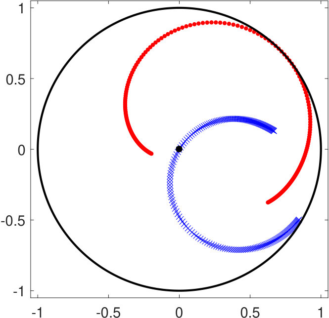 Figure 2
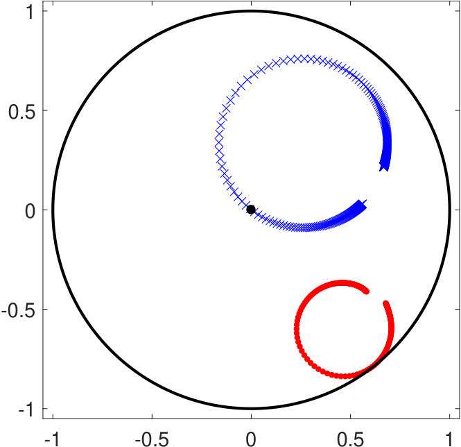 Figure 3
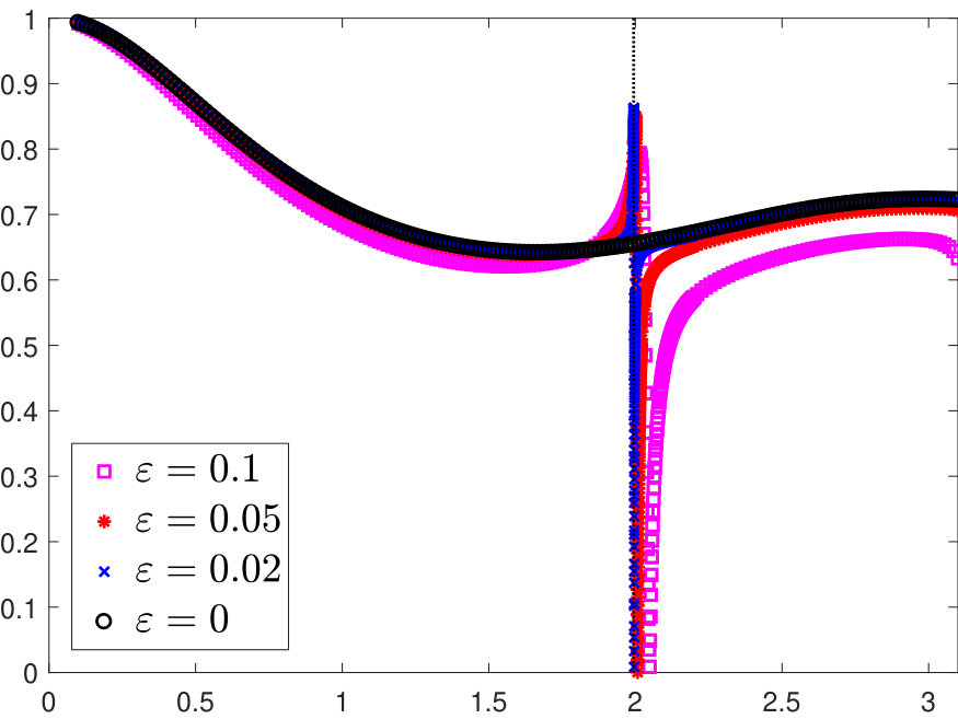 Figure 4
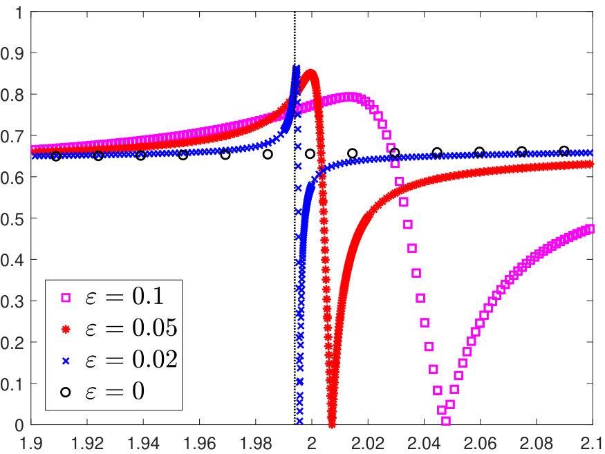 Figure 5
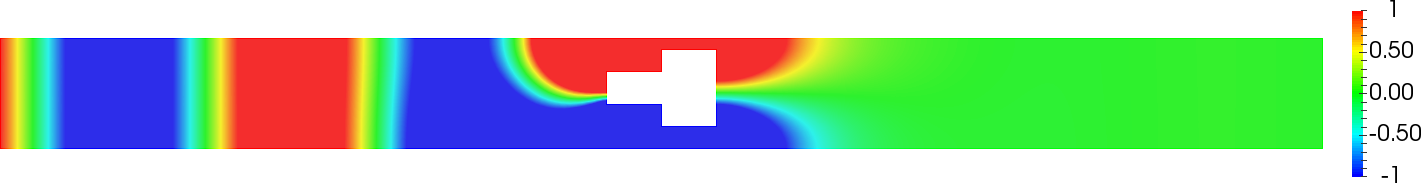 Figure 6
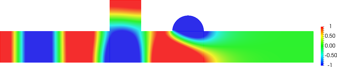 Figure 7
 Figure 8
Peer Reviews
No public reviews on file for this paper yet. If you reviewed it on a platform where reviews are public (OpenReview, ICLR, NeurIPS, ICML), you can paste yours below so the community can read it here.
Videos
No videos yet. Explain this paper in a talk, walkthrough, or lecture? Add one.
Taxonomy
TopicsPhotonic and Optical Devices · Gyrotron and Vacuum Electronics Research · Mechanical and Optical Resonators
**Exact zero transmission during the Fano resonance
phenomenon in non symmetric waveguides**
Lucas Chesnel1, Sergei A. Nazarov2
1 INRIA/Centre de math matiques appliqu es, École Polytechnique, Universit Paris-Saclay, Route de Saclay, 91128 Palaiseau, France;
2 St. Petersburg State University, Universitetskaya naberezhnaya, 7-9, 199034, St. Petersburg, Russia;
E-mails: [email protected], [email protected], [email protected]
(March 13, 2024)
Abstract. We investigate a time-harmonic wave problem in a waveguide. We work at low frequency so that only one mode can propagate. It is known that the scattering matrix exhibits a rapid variation for real frequencies in a vicinity of a complex resonance located close to the real axis. This is the so-called Fano resonance phenomenon. And when the geometry presents certain properties of symmetry, there are two different real frequencies such that we have either or , where and denote the reflection and transmission coefficients. In this work, we prove that without the assumption of symmetry of the geometry, quite surprisingly, there is always one real frequency for which we have . In this situation, all the energy sent in the waveguide is backscattered. However in general, we do not have in the process. We provide numerical results to illustrate our theorems.
Key words. Waveguides, Fano resonance, zero transmission, scattering matrix.
1 Introduction
The Fano resonance is a universal phenomenon in physics which appears in many areas. For a general presentation, we refer the reader to [18] for the seminal paper and to [27, 26] for recent reviews. In this work, we consider its expression on a model problem of propagation of time-harmonic waves in a waveguide which is unbounded in one direction. This problem appears naturally for instance in acoustics, in water-waves theory or in electromagnetism. In this context, the Fano resonance mechanism can be described as follows. Assume that the Neumann Laplacian (for the problem we consider below) has a real eigenvalue embedded in the continuous spectrum. In this case, the corresponding eigenfunctions are the so-called trapped modes which are exponentially decaying at infinity. Then perturbing slightly the setting, for example the geometry or the material index, in general this real eigenvalue will turn into a complex resonance [2, 45, 36]. And for real spectral parameters (proportional to the square of the frequency) varying in a neighbourhood of , the scattering matrix will exhibit a rapid variation. This variation is even quicker as the imaginary part of the complex resonance is small. When is between the first and the second thresholds in the continuous spectrum, so that only two conjugated waves can propagate in the waveguide, the symmetric scattering matrix is composed of two reflection coefficients , and one transmission coefficient (see the notation in (3)). In this case, under certain properties of symmetry of the configuration, one can show that the scattering coefficients take zero values for some real around . Such particular values for , are studied in particular in the context of Perfect Transmission Resonances (PTRs), see e.g. [39, 38, 24, 44, 28]. For the presentation of simple models in optics explaining the Fano resonance phenomenon, we refer the reader to [16, 17]. For more mathematical approaches, one can consult [41, 40, 42, 1, 7]. For computations of complex resonances and numerical investigations of the Fano resonance phenomenon in waveguides, we refer the reader to [12, 6, 13, 19, 21, 20]. For results concerning the existence of trapped modes associated with eigenvalues embedded in the continuous spectrum, see e.g. [43, 14, 15, 11, 25, 29, 34, 35]. Finally, note that another approach to get rigorously a zero transmission coefficient can be found in [8, 9, 10].
The goal of this note is to show that without assumption of symmetry of the configuration, the transmission coefficient still takes the zero value throughout the Fano resonance phenomenon. This was intuited in [23] using a continuation idea from a symmetric setting. In the present work, we prove rigorously the result using a different approach which does not require to start from a symmetric setting. The outline of the article is as follows. First we present the setting in Section 2. Then we perturb the geometry and the frequency of the configuration supporting trapped modes via a small parameter and we recall the results of [7] providing an asymptotic expansion of the scattering matrix with respect to tending to zero. In Section 4, we show that miraculously (we have no physical explanation for that), the main asymptotic term in the expansion of the transmission coefficient passes through zero for real around . Then in Section 5, working as in [10], we demonstrate that the unitary structure of the scattering matrix is enough to deduce that the transmission coefficient itself passes through zero for real around . We provide some numerical results to illustrate this analysis in Section 6. Finally, we give short concluding remarks. The main result of this work is Theorem 5.1.
2 Setting
Let be a domain, that is a connected open set, with Lipschitz boundary which coincides with the reference strip
[TABLE]
for where is fixed (see Figure 1). We assume that the propagation of time-harmonic waves in is governed by the Helmholtz equation with Neumann boundary conditions
[TABLE]
In this problem, is the quantity of interest (acoustic pressure, velocity potential, component of the electromagnetic field,…), denotes the 2D Laplace operator, is a parameter which is proportional to the square of the frequency and stands for the normal unit vector to directed to the exterior of . Note that from time to time, abusively we will call the frequency. We emphasize that we consider an academic problem only to simplify the presentation. Other configurations can be dealt with in a completely similar way. In particular, the analysis is the same in higher dimension and in waveguides for which the two unbounded branches are not aligned. Moreover, we can also impose Dirichlet or periodic boundary conditions in (1) to study quantum waveguides or gratings. For , only the plane waves defined by
[TABLE]
can propagate in . For , the problem (1) has solutions admitting the decompositions
[TABLE]
Here are reflection coefficients and , which is the same both for and due to the reciprocity relation, is the transmission coefficient. Moreover, the dots stand for remainders in which decay as when . Physically, (resp. ) models the scattering of the incident rightgoing wave (resp. leftgoing wave ) by the perturbation in the geometry with respect to the reference strip . We define the scattering matrix
[TABLE]
It is a classical exercise to show that is unitary () and symmetric (). The functions are uniquely defined if and only if trapped modes (non-zero solutions of (1) which are in ) do not exist at the chosen . If trapped modes exist, we define uniquely as the functions admitting the expansions (3) and which are orthogonal to the linear space of trapped modes (which is of finite dimension) in .
We assume that the geometry is such that is a simple eigenvalue of the Neumann Laplacian. In other words, we assume there is a non zero satisfying in , on and that any solution of (1) is proportional to . Note that since the continuous spectrum of the Neumann Laplacian in is , the eigenvalue is embedded in . To set ideas, we impose that . Using decomposition in Fourier series, we obtain the expansion
[TABLE]
where is a constant and is a remainder which decays as when . We assume that has a slow decay as , i.e. . In case , the analysis below must be adapted but can be done. Without lost of generality, we can impose that . Note that the choice of making an assumption on the decay of as is arbitrary. Considering the change , the analysis below can be developed completely similarly imposing the behaviour as .
3 Perturbation of the frequency and of the geometry
Now, we perturb slightly the original setting supporting trapped modes. First, the spectral parameter is changed for
[TABLE]
where is given and is small. Second, we make a perturbation of amplitude of the geometry to change into some new waveguide . More precisely, consider a smooth arc. In a neighbourhood of , we introduce natural curvilinear coordinates where is the oriented distance to such that outside and is the arc length on . Additionally, let be a smooth profile function which vanishes in a neighbourhood of the two endpoints of . Outside , we assume that coincides with and inside , is defined by the equation
[TABLE]
In other words if is parametrized as where is a given interval of , then . Here is the unit vector normal to at point directed to the exterior of . Finally we consider the perturbed problem
[TABLE]
where stands for the normal unit vector to directed to the exterior of . We denote by
[TABLE]
the scattering parameters introduced in the previous section in the geometry at frequency . And for short, we set
[TABLE]
To recall the Theorem 5.1 of [7] describing the behaviour of the scattering matrix as goes to zero, and which will be the basis of our analysis below, we need to introduce a few quantities. Set where are the functions introduced in (3) for . Set also
[TABLE]
Theorem 3.1**.**
* Assume that . Then we have*
[TABLE]
* Assume that is such that . Then we have*
[TABLE]
with and for some unimportant real constants , with . We emphasize that , are independent of , .
Let us comment this result. The methodology to prove it is the following. First, we compute an asymptotic expansion of an auxiliary object called the augmented scattering matrix, which has been introduced in [37, 22] and [30, 32] as . The essential property is that this augmented scattering matrix considered as a function of is smooth at . The procedure and the proof of error estimates are detailed in [31, 32, 33]. Then using the relation existing between the usual scattering matrix and the augmented scattering matrix, we can get the statement of the theorem.
As explained in [7], Theorem 3.1 shows that the scattering matrix is not continuous at the point (setting where trapped modes exist). Indeed, the function valued on different parabolic paths (see Figure 3) have different limits when tends to zero. And for small fixed, the usual scattering matrix exhibits a quick change in a neighbourhood of . Indeed, the map has a large variation for for some arbitrary (which is only a small change for ). Said differently, a change of order of the frequency leads to a change of order one of the scattering matrix. This is nothing but the the Fano resonance phenomenon. For a given , outside an interval of length centred at , is approximately equal to .
Remark 3.1**.**
When is such that , in general a fast Fano resonance phenomenon appears. More precisely, for a given small, the variation of of order one occurs on a range of frequencies of length (instead of when ). We write “in general” because we can also show that for well-chosen geometric perturbations, obtained solving a fixed-point problem, no Fano resonance phenomenon happens and the real eigenvalue embedded in the continuous spectrum keeps this property instead of becoming a complex resonance. In particular, this latter result allows one to construct non symmetric waveguides with eigenvalues embedded in the continuous spectrum (see [32, 33]).
From now, we denote by , the two components of , so that , and we set
[TABLE]
With this notation, the analysis developed in [7] provides the estimate
[TABLE]
where in (12), for any compact set , the constant can be chosen independent of . In particular, we have
[TABLE]
In order to prove that we have for some for small enough, we first show that the map vanishes in . This is the object of the next section.
4 Asymptotic behaviour of the transmission coefficient
Proposition 4.1**.**
Assume that . Then we have
[TABLE]
where is a circle passing through and zero.
Proof.
Classical results concerning the Möbius transform guarantee that coincides with where is a circle passing through . Let us show that also passes through zero. From (12), one finds that for some if and only if there holds
[TABLE]
In order to establish (21), we need to derive some relations between and . To proceed, first we notice that satisfies
[TABLE]
Indeed, the first component of is equal to and using (3), one finds that this function admits the expansion
[TABLE]
From the unitarity of , we infer that has the same expansion as at infinity. Using that are orthogonal to in , we deduce that . Similarly, we show that , which allows us to conclude to (14). Now we exploit (14) to establish the identity
[TABLE]
From the expressions (8)-(10) of , , and the properties of , we obtain
[TABLE]
Then replacing by (identity (14)) in , we get . This proves (15) or equivalently
[TABLE]
Finally, we use (16) to establish (21). The unitarity of imposes . Inserting this relation in the second line of (16) gives
[TABLE]
The first line of (16) implies
[TABLE]
Inserting (18) in (17) and multiplying by leads to
[TABLE]
This is identity (21). ∎
Remark 4.1**.**
The reason why passes through zero is quite mysterious. When , are symmetric with respect to the axis, this can be shown quite simply working with half-waveguides problems (see e.g. [7]). But without assumption of symmetry, we cannot provide a physical interpretation of this fact.
Denote the value of such that and for , define the interval . From (12), for small, we know that the curve
[TABLE]
passes close to zero. It remains to show that passes exactly through zero for small enough.
5 Exact zero transmission
Now, we state and prove the main result of the article. Its proof relies on Proposition 4.1 and an argument presented in [10] (see also [23]).
Theorem 5.1**.**
Assume that . Then there is such that for all , there exists such that .
Proof.
Let us first give the general idea of the proof. Assume by contradiction that for all , does not pass through zero in . Since is unitary, there holds and so
[TABLE]
But if does not pass through zero on , using Proposition 4.1 one can verify that the point must run rapidly on the unit circle for as . On the other hand, tends to a constant in as . This way we obtain a contradiction. We emphasize that the unitary structure of is the key ingredient of this step of the proof. Now we make this discussion more rigorous.
Since the circle passes through zero, there is such that is tangent to the line . Define the quadrants
[TABLE]
see Figure 4. The graph of the map crosses both quadrants and in . On the other hand, we have where is independent of for all . As a consequence, there is such that for all , the graph of the map intersects both and on .
If does not vanish in , since is continuous, we deduce that for all , there are such that and , with , . Taking successively , in the relation preceding (19), we obtain
[TABLE]
Introduce the functions such that
[TABLE]
From (11), we know that there is such that, for all , we have
[TABLE]
where for , denotes the open disk of of radius centred at . From (20), we deduce that we must have both
[TABLE]
This is impossible for small enough because (remember that ). Thus, we deduce that for all , cancels in . ∎
Concerning the zeros of , we can make the following comments. When tends to zero, from (11), we know that the curve gets closer and closer to . The set is a circle. It passes through zero if and only if we have
[TABLE]
Dividing the first line of (16) by and computing the square of the modulus, we obtain the identity
[TABLE]
Using the above equality, we obtain that (21) is satisfied if and only if there holds
[TABLE]
As a consequence, if , for small enough, does not pass through zero. Using the definition of in Theorem 3.1, we observe that we have if and are symmetric with respect to the axis. However, surely it is not necessary to consider symmetric geometries to have (22). But we emphasize that if (22) holds in a non symmetric setting, then we cannot work as in the proof of Theorem 5.1 to get exactly for some . Everything lies in the fact that the identity (19) cannot be exploited similarly for the reflection and the transmission coefficients. Therefore, a priori nothing guarantees that exact zero reflection occurs during the Fano resonance phenomenon in a non symmetric waveguide, even when (22) is satisfied.
6 Numerical results
In this section, we illustrate the results obtained above. In the first series of experiments, we work in the geometry
[TABLE]
pictured in Figure 5 left. In the obstacle is symmetric with respect to the line . According to the results of the literature (see e.g. [15]), we know that there are trapped modes for certain real frequencies in this geometry. Using Perfectly Matched Layers [4, 3, 5], we find that they exist for . Figure 5 right represents such a trapped mode in .
The domain is obtained from by shifting by the obstacle along the axis. Admittedly, this kind of perturbation is not exactly the one considered in (6). However, since there exists an almost identical mapping from to , results are similar. We emphasize that for , has no symmetry property. In Figure 6, we display the values of the complex scattering coefficients , appearing in the decomposition (3) of for and for (note that this interval contains the value ). To proceed, we use a finite element method in a truncated geometry. On the artificial boundary created by the truncation, a Dirichlet-to-Neumann operator with terms serves as a transparent condition. As expected, we observe that passes through zero.
In Figure 7, we display the curves for several and a range of values of . The right picture is a zoom of the left picture around . As expected we observe that for the different , we have for one close to . We also note that the smaller is, the faster the Fano resonance phenomenon occurs. This is also expected. Finally, in Figure 8, we display the real part of (see (3)) in for and . In this setting, there holds . And indeed we observe that the incident rightgoing wave is completely backscattered, this is the mirror effect.
In the second series of experiments, we work in the geometry of Figure 10. Using Perfectly Matched Layers, we find a complex resonance such that . In Figure 9, we display the values of the complex scattering coefficients , appearing in the decomposition (3) of for (note that this interval contains the value ). Though this experiment does not strictly enter the framework presented in this note (we do not start from a situation where trapped modes exist), we observe that the curve passes through zero for in a neighbourhood of . In Figure 10, we display the real part of for . In this setting, we have .
7 Concluding remarks
In this note, we proved that during the Fano resonance phenomenon in monomode regime, without assumption of symmetry of the geometry, the transmission coefficient passes through zero. Physically, when the transmission coefficient is null, the energy of an incident wave propagating through the structure is completely backscattered. As already mentioned, everything presented here is also valid in higher dimension and with Dirichlet or periodic boundary conditions instead of Neumann ones. We considered a geometrical perturbation of the walls of the waveguide. We could also have worked with a penetrable inclusion placed in the waveguide. Then perturbing the material parameter, we would have obtained similar results. Importantly, the above analysis applies only in monomode regime, that is for our geometry when belongs to . It is not clear what happens in multimodal regime (. Moreover, we assumed that is a simple eigenvalue embedded in the continuous spectrum of the Neumann Laplacian. When is not simple, the analysis has to be done.
Acknowledgments
The research of S.A. Nazarov was supported by the grant No. 17-11-01003 of the Russian Science Foundation.
The reference list from the paper itself. Each links out to its DOI / PubMed record.
- 1[1] G.S. Abeynanda and S.P. Shipman. Dynamic resonance in the hign-Q and near-monochromatic regime. In MMET, IEEE , pages 102–107, 2016.
- 2[2] A. Aslanyan, L. Parnovski, and D. Vassiliev. Complex resonances in acoustic waveguides. Quart. J. Mech. Appl. Math. , 53(3):429–447, 2000.
- 3[3] E. Bécache, A.-S. Bonnet-Ben Dhia, and G. Legendre. Perfectly matched layers for the convected helmholtz equation. SIAM J. Numer. Anal. , 42(1):409–433, 2004.
- 4[4] J.-P. Berenger. A perfectly matched layer for the absorption of electromagnetic waves. J. Comput. Phys. , 114(2):185–200, 1994.
- 5[5] A.-S. Bonnet-Ben Dhia, L. Chesnel, and V. Pagneux. Trapped modes and reflectionless modes as eigenfunctions of the same spectral problem. Proc. R. Soc. A , 474(2213):20180050, 2018.
- 6[6] G. Cattapan and P. Lotti. Fano resonances in stubbed quantum waveguides with impurities. Eur. Phys. J. B , 60(1):51–60, 2007.
- 7[7] L. Chesnel and S.A. Nazarov. Non reflection and perfect reflection via Fano resonance in waveguides. Comm. Math. Sci. , 16(7):1779–1800, 2018.
- 8[8] L. Chesnel, S.A. Nazarov, and V. Pagneux. Invisibility and perfect reflectivity in waveguides with finite length branches. SIAM J. Appl. Math. , 78(4):2176–2199, 2018.