Mahler measures of a family of non-tempered polynomials and Boyd's conjectures
Yotsanan Meemark, Detchat Samart

TL;DR
This paper establishes a new identity linking Mahler measures of non-tempered and tempered polynomials, evaluates some Mahler measures via special functions, and proves Boyd's conjectures for certain elliptic curves.
Contribution
It introduces a novel identity connecting Mahler measures of different polynomial families and confirms Boyd's conjectures for conductor 30 elliptic curves.
Findings
Derived an identity relating Mahler measures of non-tempered and tempered polynomials.
Expressed Mahler measures in terms of special values of L-functions and logarithms.
Proved Boyd's conjectures for conductor 30 elliptic curves.
Abstract
We prove an identity relating Mahler measures of a certain family of non-tempered polynomials to those of tempered polynomials. Evaluations of Mahler measures of some polynomials in the first family are also given in terms of special values of -functions and logarithms. Finally, we prove Boyd's conjectures for conductor elliptic curves using our new identity, Brunault-Mellit-Zudilin's formula and additional functional identities for Mahler measures.
Click any figure to enlarge with its caption.
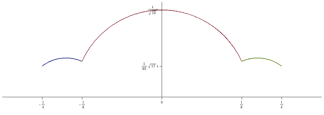 Figure 1
Peer Reviews
No public reviews on file for this paper yet. If you reviewed it on a platform where reviews are public (OpenReview, ICLR, NeurIPS, ICML), you can paste yours below so the community can read it here.
Videos
No videos yet. Explain this paper in a talk, walkthrough, or lecture? Add one.
Mahler measures of a family of non-tempered polynomials and Boyd’s conjectures
Yotsanan Meemark
Department of Mathematics and Computer Science, Faculty of Science, Chulalongkorn University, Bangkok, Thailand 10330
and
Detchat Samart
Department of Mathematics, Faculty of Science, Burapha University, Chonburi, Thailand 20131
Abstract.
We prove an identity relating Mahler measures of a certain family of non-tempered polynomials to those of tempered polynomials. Evaluations of Mahler measures of some polynomials in the first family are also given in terms of special values of -functions and logarithms. Finally, we prove Boyd’s conjectures for conductor elliptic curves using our new identity, Brunault-Mellit-Zudilin’s formula and additional functional identities for Mahler measures.
In memory of John Tate
1. Introduction
The (logarithmic) Mahler measure of a nonzero -variate Laurent polynomial is defined by
[TABLE]
Before stating the problems to be investigated in this article, let us recall the definition of a tempered polynomial in two variables [25, Sect. III].
Definition 1**.**
Let and let be the Newton polygon of . For each side of , we denote the lattice points on (enumerated clockwise) by . Then we associate to the univariate polynomial
[TABLE]
(Note that this is a finite sum since only a finite number of are non-zero.) The polynomial is said to be tempered if, for every side of , the zeroes of are roots of unity. Otherwise, is non-tempered.
In this paper, we mainly study Mahler measures of the following -parametric family of Laurent polynomials:
[TABLE]
It is clear from Definition 1 that, for , is tempered if and only if . In his seminal paper [5], Boyd verified numerically that for many integral values of
[TABLE]
where , is the elliptic curve corresponding to and means the two quantities are equal to at least decimal places. The numerical values of and can be computed rapidly with high precision using standard computer algebra systems such as Mathematica and Magma, yet the identity (1.2) is notoriously difficult to prove in general. In [16], Lalín, Zudilin, and the second author establish an identity relating , for , to ‘half-Mahler’ measures of , where and are algebraic expressions of and use it to prove Boyd’s conjecture
[TABLE]
where has conductor . The (conjectural) equation (1.2) is in fact an instance of a more general conjecture, namely the Bloch-Beilinson conjecture, which predicts a deep connection between regulators and -functions associated to algebraic varieties. The link between this conjecture and Mahler measures was first observed by Deninger [9] and was examined extensively by Boyd and Rodriguez Villegas [5, 25]. Another example of tempered polynomials is the family
[TABLE]
Boyd [5, Tab. 2] found that appears to satisfy an identity analogous to (1.2) for many . Again, due to the limitedness of the known techniques, only a handful of these identities have been proven rigorously, as shown in Table 1.
Temperedness of a two-variable polynomial has certain -theoretic interpretation which potentially leads to a conjecture like (1.2). In fact, if is a tempered polynomial defining an elliptic curve , then is expressible in terms of a regulator integral
[TABLE]
where is a path on . (For more details, the reader is referred to [9, 25].) Non-tempered polynomials, on the other hand, are less well understood. Boyd’s experiment showed that Mahler measures of some non-tempered polynomials in two variables are (conjecturally) -linear combinations of logarithms and -values. For example, he found
[TABLE]
for some and and hypothesized that the logarithmic term arises from the Mahler measure of , which corresponds to a side of the Newton polygon of . The first proven formula in this family (with and ) was given recently by Lalín and Ramamonjisoa [18]. Examples of proven Mahler measure formulas for non-tempered polynomials involving logarithms and -values can be found in [15, 12]. Due to the sparsity of the known results, it is of great importance to gain further examples of non-tempered polynomials whose Mahler measures encode interesting arithmetic information like (1.4).
In the last section of [16], the following identity is stated without proof: for every
[TABLE]
The primary goal of this paper is to give a proof of an extended version of this statement.
Theorem 2**.**
If , then the following identity holds:
[TABLE]
This result, which is proven in Section 2, gives a direct connection between Mahler measures of a non-tempered family and those of a tempered family. Note also that and generically define the same elliptic curve (up to isomorphism), which can be written in a Weierstrass form as
[TABLE]
Using Theorem 2 and the proven identities in Table 1, we immediately obtain some new formulas for which are analogous to (1.4).
Corollary 3**.**
The following evaluations are true:
[TABLE]
Many recent results relating Mahler measures of two-variate polynomials to elliptic curve -values are accomplished using elegant formulas of Brunault, Mellit and Zudilin [26, 7]. However, these formulas are applicable only for finitely many elliptic curves over , which admit a modular unit parametrization [6]. Indeed, the motivation for studying the family is the existence of modular units parametrizing , which is equivalent to a classical result of Ramanujan. This eventually leads to a proof of (1.3). In Section 3 and Section 4, we use a similar approach to tackle Boyd’s conjectures for elliptic curves of conductor [5, Tab. 2], including
[TABLE]
Note that there is only one isogeny class of conductor elliptic curves, so the -values on the right-hand sides of (1.6), (1.7) and (1.8) all coincide. To prove these formulas, we first use a newly-discovered modular unit parametrization for and Brunault-Mellit-Zudilin’s formula to establish a formula for .
Theorem 4**.**
The following formula holds:
[TABLE]
It is clear that (1.6) follows from (1.5) and (1.9). The remaining two formulas can be deduced by comparing the Mahler measures in the level of regulator via isogenies or isomorphisms between elliptic curves. The details of the proof will be given in Section 4. In the end, we are able to settle all conjectural identities of Boyd in conductor .
Theorem 5**.**
The formulas (1.6), (1.7) and (1.8) are true.
It is worth mentioning that Rogers and Yuttanan made some observations about the conductor conjectures in [21] by expressing the -value in terms of certain lattice sums. Using Theorem 5, we are able to confirm all of their related conjectures. For example, we have
[TABLE]
where
[TABLE]
2. Proof of Theorem 2
We follow an approach of Bertin and Zudilin [2] in proving Theorem 2. The crucial idea is to compare the derivatives of and with respect to the real parameter (or if ). These quantities turn out to be expressible in terms of elliptic integrals, which can be manipulated quite easily by changing variables. We divide the proof into two parts, depending on whether is real or purely imaginary.
For the sake of brevity, denote
[TABLE]
We will also make use of the following standard notations for complete elliptic integrals:
[TABLE]
2.1. The real cases
Lemma 6**.**
For , we have
[TABLE]
where and .
Proof.
We denote
[TABLE]
By the quadratic formula, we have
[TABLE]
where If , then and have modulus and are complex conjugates of each other, since . Otherwise, we let
[TABLE]
so that
By Jensen’s formula and the fact that , we obtain
[TABLE]
Note that , since . If , then , so using
[TABLE]
and , one sees that . Therefore,
[TABLE]
Simple calculations yield
[TABLE]
It follows that
[TABLE]
Then we use the substitution to obtain
[TABLE]
Note that the above integral converges for . Using the change of variable
[TABLE]
one can check easily that
[TABLE]
where and . Substituting (2.2) and (2.3) into (2.1) proves the lemma. ∎
Lemma 7**.**
For , we have
[TABLE]
where .
Proof.
It is proven in [2, Sect. 3] that the derivative of can be written in terms of a hypergeometric function. In particular, we have
[TABLE]
for any . Assume first that . Using the substitution , we have , so we can apply [1, p. 112, Thm. 5.6] to deduce
[TABLE]
where the last equality follows from the standard hypergeometric representation of .
The remaining cases can be verified in a similar manner using the substitution and the identity [10, Eq. 19.7.3]
[TABLE]
which is valid for . ∎
We shall compare the derivatives of and using the preceding lemmas.
Lemma 8**.**
For , the equality
[TABLE]
holds.
Proof.
By Lemma 6, Lemma 7, and some rearrangement, it suffices to prove that, for every ,
[TABLE]
where and are as given in Lemma 6. Surprisingly, this is equivalent to a known result due to Jia [14], which arises from certain problems in particle physics. His proof is based on the observation that, after applying the change of variable the function on the left-hand side of (2.5), which he called , satisfies the first-order differential equation
[TABLE]
This can be derived using the derivative formulas for and (see [10, Chapter 19] or [16, p. 13]) and the chain rule. The solution to the above ODE defined on is
[TABLE]
where is a constant. Using some initial conditions, he found that and the proof is completed. ∎
Proof of Theorem 2 for .
The case is trivial since . Suppose . Then we have from Lemma 8 that
[TABLE]
Since and are continuous functions on , it follows that (1.5) is valid for all . ∎
Remark 9*.*
The discontinuity at in Lemma 8 is natural due to the fact that the curve is singular. In particular, the Mahler measures and are not related to elliptic curve -values. On the other hand, Boyd [5, Tab. 2] conjectured that
[TABLE]
where
2.2. The complex cases
We first simplify the problem a bit to avoid working with complex variables. Let where Then we have
[TABLE]
Since , it follows that
[TABLE]
where Here we have applied the transformation and [23, Lem. 7] to modify the Mahler measure slightly on the right-hand side. Consequently, the proof of Theorem 2 for the complex cases boils down to showing that
[TABLE]
for real . We will employ the techniques that we use in the real cases to verify (2.6).
Lemma 10**.**
Let . Then for , which is mapped bijectively to , we have
[TABLE]
where and
Proof.
Let
[TABLE]
Since , we have Hence, by the arguments used in the proof of Lemma 6,
[TABLE]
Then we differentiate both sides with respect to and do some calculations to obtain
[TABLE]
where . Note that the polynomial in the denominator has only two real roots, so the process of writing this integral in terms of elliptic integrals is more involved than that in the proof of Lemma 6. Let us first rewrite the two quadratic polynomials
[TABLE]
where
[TABLE]
Let . Then we have , whence
[TABLE]
Applying partial fraction decomposition results in
[TABLE]
Using the substitution , one sees that
[TABLE]
On the other hand, by the substitution
[TABLE]
Hence we have
[TABLE]
By the same transformation, one can easily deduce
[TABLE]
In the final step, we alter the arguments of the elliptic integrals in (2.7) and (2.8) using the following identities [10, Eq. 15.8.1, 16.16.8]:
[TABLE]
which hold whenever and . ∎
Lemma 11**.**
Under the same assumption as those in Lemma 10, we have
[TABLE]
Proof.
This is again a consequence of [2, Eq. (5)] and [1, p. 112, Thm. 5.6]. See the proof of Lemma 7 for further details. ∎
We can now give a comparison between the two derivatives in the previous two lemmas.
Lemma 12**.**
For ,
[TABLE]
Proof.
By Lemma 10 and Lemma 11, proving (2.9) amounts to verifying that the following identity is true for :
[TABLE]
where and We shall imitate Jia’s arguments, outlined in the proof of Lemma 8, to prove (2.10). Let us denote the function on the left-hand side of (2.10) by . Computing the derivatives of the two elliptic integrals yields
[TABLE]
Hence it is easily seen that satisfies
[TABLE]
This differential equation has a general solution on the interval of the form
[TABLE]
where is constant. Letting , one immediately sees
[TABLE]
and we have (2.10). ∎
Proof of Theorem 2 for .
Integrating both sides of (2.9) results in
[TABLE]
for some constant . Note that as
[TABLE]
As a consequence, as , which implies This proves (2.6), so (1.5) is valid for all ∎
3. Modular unit parametrization in level
The aim of this section is to prove Theorem 4; i.e.,
[TABLE]
Following the notation in [26], for each , we define a level modular unit as
[TABLE]
where . Let and be functions on the upper half-plane defined by
[TABLE]
where is the Dedekind eta function. In the following theorem, we will show that the curve can be parametrized by and .
Theorem 13**.**
The following identity holds:
[TABLE]
Proof.
Let . Then it can be shown using Newman’s theorem and Ligozat’s theorem [20, Thm. 1.64 and 1.65] that
[TABLE]
where denotes the space of weight modular forms for Hence we have
[TABLE]
By Sturm’s theorem [24], a weight modular form for is identically zero if its first Fourier coefficients vanish. Since
[TABLE]
we only need to show that the first twelve coefficients of are zero. These can be easily computed using a computer. ∎
Remark 14*.*
To the best of our knowledge, the modular equation (3.1) never appeared in the literature. We discovered it via a modular parametrization of the conductor elliptic curve
[TABLE]
and the transformations [16, Eq. (11)]
[TABLE]
with the aid of CoCalc [13] and qseries package in Maple [11]. Note, however, that the corresponding and are not modular unit parametrization of . It would be interesting to find one for or the curve .
Consider the following CM points
[TABLE]
We shall denote by the geodesic (a circular arc or a vertical straight line orthogonal to the -axis) connecting and . The geodesics and are illustrated in Figure 1 below.
Let us briefly explain motivation behind the construction of geodesics in Figure 1. It will be shown in the proof of Lemma 17 that can be written as an integral over a path joining two CM points on . This integral can then be transformed into an integral of functions involving and from to on , so the integration path becomes a geodesic in . The strategy is to split into smaller paths on which the value of is real in order to make the calculations simple. Based on some numerical computation, we find it suitable to divide into three geodesics as shown above.
The (normalized) Atkin-Lehner involutions
[TABLE]
of will be invoked frequently in the proofs of the subsequent lemmas, so we record them here for convenience.
Lemma 15**.**
For we have and
Proof.
Let . Then can be written in the form
[TABLE]
so Hence it can be checked easily that
[TABLE]
It follows that sends to their complex conjugates On the other hand, by [8, Cor. 2.2], we have that acts on the two modular functions as follows: . Therefore, we have and , implying and . By symmetry, it is not hard to see that the same result holds for
For , we have , whence
[TABLE]
Thus sends to . Since the action of on and is the same as that of [8, Cor. 2.2], we have the same conclusion as above. ∎
Lemma 16**.**
The following evaluations are true:
[TABLE]
Proof.
Employing the action of , we have
[TABLE]
Hence has modulus . It is clear from Lemma 15 and the definition of that Then we apply Theorem 13 to deduce that is a zero of the polynomial . It is therefore sufficient to consider the sign of numerically in order to get a correct value of The values of and can be obtained using the action of and the same arguments. ∎
For meromorphic functions and on a smooth curve , we define the real differential form on as
[TABLE]
where . Hence if and are real. Moreover, it can be shown in a straightforward manner using the definition above that is bi-additive; i.e.,
[TABLE]
Lemma 17**.**
The following identity is true:
[TABLE]
Proof.
Recall from [16, Sect. 3] that, for any real numbers and , , where is an integral of certain function in variable from to . In addition, we have that if , then
[TABLE]
where and
[TABLE]
Substituting and into these expressions, we obtain
[TABLE]
where and are points on given by
[TABLE]
Here we think of and as rational functions of and via the transformation (3.2) and integrate the differential form on the curve . The points correspond to
[TABLE]
on the curve . By Lemma 16, we have
[TABLE]
One sees from Theorem 13 and symmetry that the function can possibly be corresponding to either or . We need further information to correctly identify . On the path , we have [16, Sect. 3] and, by evaluating numerically, on . Therefore, we have
[TABLE]
where the second equality is obtained by splitting the path into and using (3.3) and the fact proven in Lemma 15 that is real on these paths. It should be noted that we are able to decompose the integration path in freely since the singularities of and are confined to the cusps.
The action of the involution results in and [8, Cor. 2.2]. Thus sends to We also have that sends to and [math] to . Consequently,
[TABLE]
Observe that is real on and , so by splitting into the union of these three paths one sees that
[TABLE]
Plugging this back into the last expression above, we have
[TABLE]
where the last equality follows from the fact that both and are real on ∎
We are now in a good position to apply the following formula of Brunault and Mellit, whose proof is worked out in detail by Zudilin [26], in order to prove Theorem 4.
Theorem 18** (Brunault-Mellit-Zudilin).**
Let be a positive integer and define
[TABLE]
where . Then for any such that and ,
[TABLE]
where is a weight modular form given by
[TABLE]
and
[TABLE]
Proof of Theorem 4.
Let be the normalized newform corresponding to the elliptic curve via the modularity theorem and let be the normalized weight Eisenstein series; i.e.,
[TABLE]
(The reader should be warned not to confuse with the curve in the remaining part of this proof.) Using Lemma 17, Eq. (3.3), and Theorem 18, we have
[TABLE]
where
[TABLE]
Note that and the Eisenstein series in the above expression belong to . Using Sturm’s theorem, we obtain this identification for by comparing the first twelve Fourier coefficients of both sides. Hence is a rational linear combination of an -value of and those of Eisenstein series. For , we have
[TABLE]
Therefore, if , then
[TABLE]
where
[TABLE]
The Laurent series of and around are
[TABLE]
implying . In summary, we have
[TABLE]
Finally, we apply the standard functional equation for to acquire the desired result. ∎
4. Elliptic regulator and proof of Theorem 5
In this section, we will establish relationships between and using their connection with the regulator map on the second -group of the corresponding elliptic curve. We start by recalling some notations and definitions which will be used throughout this section. For more details, the reader is referred to [25].
Let be an elliptic curve defined over and let be its function field. Note that the first cohomology group can be viewed as the dual of the group of homologous cycles . With this identification, the regulator map is defined by
[TABLE]
for [3, 4]. If is defined over , then is conjectured to be a finitely generated abelian group of positive rank, though it is difficult to compute explicitly in general. However, under certain conditions, which are satisfied by curves defined by tempered polynomials, we can identify each element of by that of . On the other hand, Matsumoto’s theorem yields
[TABLE]
Since for some , we can write each point on as , with . The regulator function , originally defined by Bloch [4], is given by
[TABLE]
where the summation excludes . Observe that can be extended linearly to the set of divisors on .
Let be the set of equivalence classes of divisors on under the relation . The diamond operation is defined by
[TABLE]
Following notations in many previous papers, we set
[TABLE]
Recall from Section 1 that the curve is birational to
[TABLE]
Using Jensen’s formula and work of Deninger and Rodriguez Villegas [9, 25], one can rewrite as
[TABLE]
where corresponds to a path on subject to the conditions and . Following this approach, Mellit [19] proved that
[TABLE]
and corresponds to Lalín then applied the regulator machinery to establish the following functional identity [17, Thm. 1.1]: for ,
[TABLE]
The particular cases and of (4.2) can be written as
[TABLE]
implying
[TABLE]
Therefore, knowing a relationship between and any of would be adequate to settle the conductor conjectures. Since there are no known functional identities that give such a relationship directly, we will show that it exists by adapting arguments in the proof of [17, Thm. 1.1].
Theorem 19**.**
The following identity is valid:
[TABLE]
Proof.
For consistency between our notations and those in [17], we define the elliptic curve by
[TABLE]
We have a birational map from the curve to via the change of variables
[TABLE]
The torsion subgroup of has a cyclic subgroup of order generated by . If , then also has a point of order which is independent of , namely . Lalín showed that
[TABLE]
Moreover, setting and , she used the isomorphisms
[TABLE]
to obtain
[TABLE]
For our purposes, we choose so that the above isomorphisms become and and for convenience we shall write and , , for the corresponding functions on , and , respectively. The torsion subgroup of is generated by and and the base point of at infinity will be denoted by . We have from the two equations above that
[TABLE]
Consider the rational functions
[TABLE]
on the curve . Their divisors are
[TABLE]
where and . Applying the diamond operation yields
[TABLE]
It follows that
[TABLE]
Since and are trivial in -theory, we have
[TABLE]
Putting (4.4), (4.5), and (4.6) together, we obtain
[TABLE]
Finally, we apply the regulator function and use (4.1) to translate the above identity into
[TABLE]
as desired. ∎
Proof of Theorem 5.
By (1.5), (1.9), (4.3), and Theorem 19, we have
[TABLE]
Since the curves and are in the same isogeny class, the proof is complete. ∎
5. Concluding remarks
The -parametric family apparently has some interesting arithmetic properties. If we choose properly to be an algebraic expression of , their Mahler measures (or half-Mahler measures) turn out to be related to those of the one-parametric tempered families and , as one can see from [16, Thm. 2] and Theorem 2 in this article. A key feature of these results is that they can be applied to obtain rigorous proofs for some conjectures of Boyd concerning and . The proofs of the two theorems mentioned above rely on, after some manipulations, the existence of identities between the complete elliptic integrals of the first and the third kind. It might be possible to recover other functional identities for Mahler measures by tracking backwards from elliptic integral identities similar to (2.5) and (2.10). It would also be desirable to prove Boyd’s other conjectures using modular equations in different levels.
Acknowledgements This research is supported financially by the Thailand Research Fund (TRF) grant from the TRF and the Office of the Higher Education Commission, under the contract number MRG6280045. Part of this work was done during the second author’s visit to the Vietnam Institute for Advanced Study in Mathematics (VIASM) in the Summer semester of year 2018, partially supported under the institute’s research contract no. NC/2018/VNCCCT. The second author is grateful to the VIASM for their support and hospitality. The authors would like to thank Bruce Berndt and Wadim Zudilin for their valuable comments on an earlier version of this paper. Lastly, the authors thank the anonymous referee for insightful remarks which greatly help to improve the exposition of this paper and for a suggestion about possible approach to completing the proof of Boyd’s conductor conjectures.
The reference list from the paper itself. Each links out to its DOI / PubMed record.
- 1[1] Bruce C. Berndt, Ramanujan’s notebooks. Part V , Springer-Verlag, New York, 1998. MR 1486573
- 2[2] Marie José Bertin and Wadim Zudilin, On the Mahler measure of a family of genus 2 curves , Math. Z. 283 (2016), no. 3-4, 1185–1193. MR 3519999
- 3[3] A. A. Beĭlinson, Higher regulators and values of L 𝐿 L -functions of curves , Funktsional. Anal. i Prilozhen. 14 (1980), no. 2, 46–47. MR 575206
- 4[4] Spencer J. Bloch, Higher regulators, algebraic K 𝐾 K -theory, and zeta functions of elliptic curves , CRM Monograph Series, vol. 11, American Mathematical Society, Providence, RI, 2000. MR 1760901
- 5[5] David W. Boyd, Mahler’s measure and special values of L 𝐿 L -functions , Experiment. Math. 7 (1998), no. 1, 37–82. MR 1618282
- 6[6] François Brunault, Parametrizing elliptic curves by modular units , J. Aust. Math. Soc. 100 (2016), no. 1, 33–41. MR 3436769
- 7[7] by same author, Regulators of Siegel units and applications , J. Number Theory 163 (2016), 542–569. MR 3459587
- 8[8] Heng Huat Chan and Mong Lung Lang, Ramanujan’s modular equations and Atkin-Lehner involutions , Israel J. Math. 103 (1998), 1–16. MR 1613532