Minimizing the expected value of the asymmetric loss and an inequality of the variance of the loss
Naoya Yamaguchi, Yuka Yamaguchi, and Ryuei Nishii

TL;DR
This paper proposes a method to adjust predictions to minimize the expected asymmetric loss and variance of the loss, without estimating regression coefficients, by ensuring the prediction error follows a normal distribution.
Contribution
It introduces a novel approach that corrects predictions to optimize asymmetric loss and variance without traditional coefficient estimation.
Findings
Effective reduction in expected asymmetric loss.
Lowered variance of prediction errors.
Applicable to various prediction scenarios.
Abstract
For some estimations and predictions, we solve minimization problems with asymmetric loss functions. Usually, we estimate the coefficient of regression for these problems. In this paper, we do not make such the estimation, but rather give a solution by correcting any predictions so that the prediction error follows a general normal distribution. In our method, we can not only minimize the expected value of the asymmetric loss, but also lower the variance of the loss.
Click any figure to enlarge with its caption.
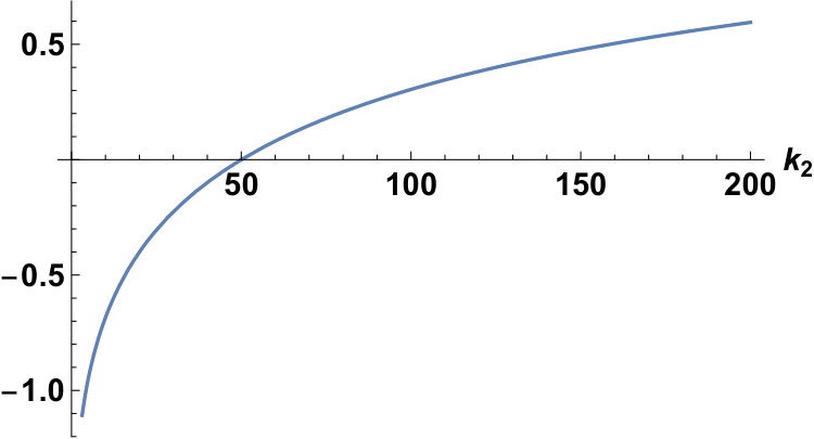 Figure 1
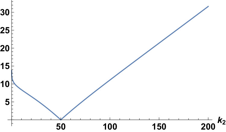 Figure 2
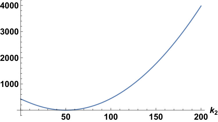 Figure 3
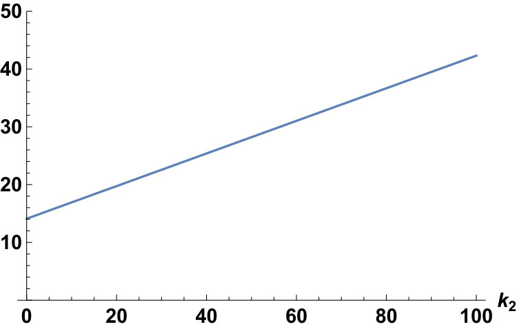 Figure 4
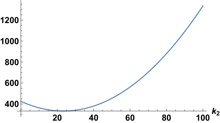 Figure 5
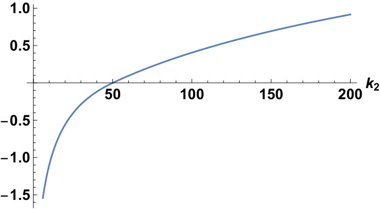 Figure 6
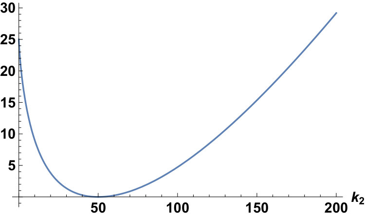 Figure 7
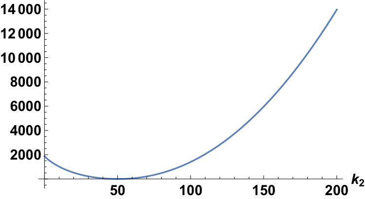 Figure 8
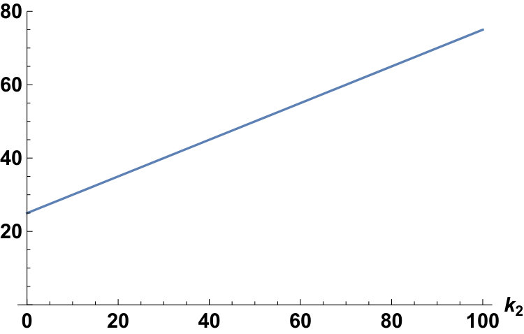 Figure 9
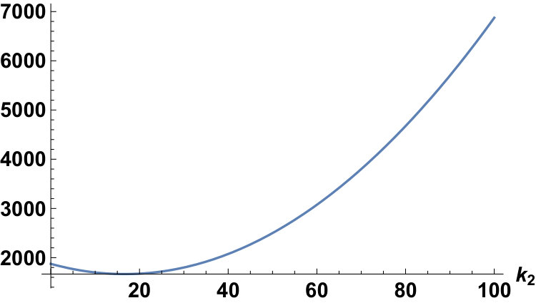 Figure 10
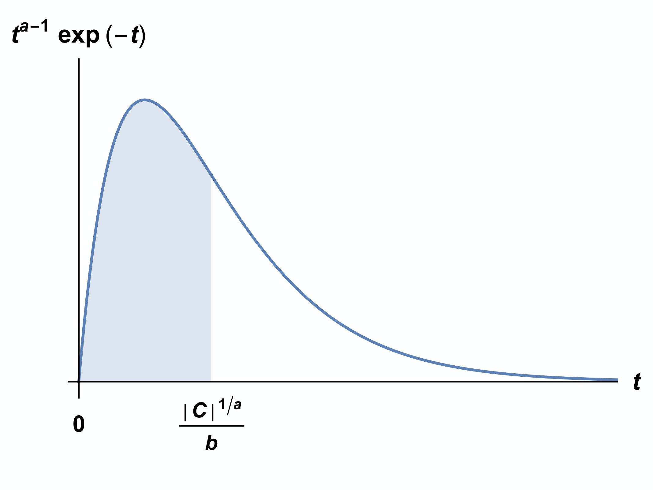 Figure 11
Peer Reviews
No public reviews on file for this paper yet. If you reviewed it on a platform where reviews are public (OpenReview, ICLR, NeurIPS, ICML), you can paste yours below so the community can read it here.
Videos
No videos yet. Explain this paper in a talk, walkthrough, or lecture? Add one.
Taxonomy
TopicsExplainable Artificial Intelligence (XAI) · Statistical Methods and Inference · Bayesian Modeling and Causal Inference
Minimizing the expected value of the asymmetric loss and an inequality of the variance of the loss
Naoya Yamaguchi, Yuka Yamaguchi, and Ryuei Nishii
Abstract.
For some estimations and predictions, we solve minimization problems with asymmetric loss functions. Usually, we estimate the coefficient of regression for these problems. In this paper, we do not make such the estimation, but rather give a solution by correcting any predictions so that the prediction error follows a general normal distribution. In our method, we can not only minimize the expected value of the asymmetric loss, but also lower the variance of the loss.
Key words and phrases:
asymmetric loss function; risk function; minimizing the expectation value; generalized Gauss distribution; gamma function.
2010 Mathematics Subject Classification:
Primary 62A99; Secondary 62E99.
1. Introduction
For some estimations and predictions, we solve minimization problems with loss functions, as follows: Let be a data set, where are vectors and . We assume that the data relate to a linear model,
[TABLE]
where , , and is the matrix having as the th row. Let be a loss function and let . Then we estimate the value:
[TABLE]
The case of is well-known (see, e.g., Refs. [1], [8], and [10]). In the case of an asymmetric loss function, we refer the reader to, e.g., Refs. [3], [5], [7], and [14]. These studies estimate the parameter . In this paper, however, we do not make such the estimation, but instead give a solution to the minimization problems by correcting any predictions so that the prediction error follows a general normal distribution. In our method, we can not only minimize the expected value of the asymmetric loss, but also lower the variance of the loss.
Let be an observation value, and let be a predicted value of . We derive the optimized predicted value minimizing the expected value of the loss under the assumption:
- (1)
The prediction error is the realized value of a random variable , whose density function is a generalized Gaussian distribution function (see, e.g., Refs. [4], [9], and [11]) with mean zero
[TABLE]
where is the gamma function and , . 2. (2)
Let , . If there is a mismatch between and , then we suffer a loss,
[TABLE]
That is, the solution to the minimization problem is
[TABLE]
The motivation of our research is as follows: (1) Predictions usually cause prediction errors. Therefore, it is necessary to use predictions in consideration of predictions errors. Actually, in some cases, it is best not to act as predicted because of prediction errors. For example, the paper [13] formulates a method for minimizing the expected value of the procurement cost of electricity in two popular spot markets: day-ahead and intra-day, under the assumption that the expected value of the unit prices and the distributions of the prediction errors for the electricity demand traded in two markets are known. The paper showed that if the procurement is increased or decreased from the prediction, in some cases, the expected value of the procurement cost is reduced. (2) In recent years, prediction methods have been black boxed by the big data and machine learning (see, e.g., Ref. [6]). The day will soon come, when we must minimize the objective function by using predictions obtained by such black boxed methods. In our method, even if we do not know the prediction , we can determine the parameter if we know the prediction error distribution and asymmetric loss function .
To obtain , we derive for any . Let and be the upper and the lower incomplete gamma functions, respectively (see, e.g., Ref. [12]). The expected value and the variance of are as follows:
Lemma 1**.**
For any , we have
[TABLE]
We write the value of satisfying as . Then, we find that has a minimum value at . Also, it follows from
[TABLE]
that , where , and only when . This equation implies that the ratio of and is . That is, the vertical axis divides the area between and the -axis into .
Substituting in the equation of Lemma 1, from the equation , we have
[TABLE]
This is the minimum value of . From this and the case of the equation of Lemma 1, we have the following corollary:
Corollary 2**.**
We have
[TABLE]
This corollary asserts that the expected value of the loss is reduced by correcting a predicted value to the optimized predicted value . Moreover, the following holds:
Theorem 3**.**
We have
[TABLE]
where equality sign holds only when ; that is, when .
This theorem asserts that the variance of the loss is reduced by correcting the predicted value to the optimized predicted value . To prove this theorem, we use the following lemma:
Lemma 4**.**
For and , we have
[TABLE]
To prove Lemma 4, we use the following lemmas:
Lemma 5**.**
For , we have
[TABLE]
Lemma 6**.**
For , we have
[TABLE]
The remainder of this paper is organized as follows. In Section , we set up the problem. In Section , we introduce the expected value and the variance of , and we determine the value of that gives the minimum value of . In addition, we give a geometrical interpretation of the parameter , and give the minimized expected value . In Section , we prove Theorem 3. In Section , we give some inequalities for the gamma and the incomplete gamma functions, which used to derive the inequality for the variance of the loss in Theorem 3. In Section , we write the calculation of the expected value and the variance of the loss for .
2. Problem statement
In this section, we set a problem. Let be an observation value, let be a predicted value of , and let be the gamma function (see, e.g., Ref. [12, p. 93]) defined by
[TABLE]
We assume the following:
- (1)
The prediction error is the realized value of a random variable , whose density function is a generalized Gaussian distribution function (see, e.g., Refs. [4], [9], and [11]) with mean zero
[TABLE]
where , . 2. (2)
Let , . If there is a mismatch between and , then we suffer a loss,
[TABLE]
We derive the optimized predicted value minimizing . For this purpose, we derive for any in the next section.
3. Expected value and variance of the loss
Here, we introduce the expected value and the variance of , and determine the value of that gives the minimum value of . In addition, we give a geometrical interpretation of the parameter and give the minimized expected value .
3.1. Expected value and variance of the loss
Let and be the upper and the lower incomplete gamma functions, respectively, defined by
[TABLE]
where and . These functions have the following properties:
Lemma 7**.**
For and ,
[TABLE]
Also, for , let . Then, the expected value and the variance of are as follows:
Lemma 8** (Section 1, Lemma 1).**
For any , we have
[TABLE]
See the last two sections for the proof of Lemma 8.
From Lemma 8, we have the following:
[TABLE]
Let be the error function defined by
[TABLE]
for any . We give two examples of and .
Example 9**.**
In the case of , since , we have
[TABLE]
In the case of , since , we have
[TABLE]
With the conditions fixed as and , we can plot and for the Laplace and the Gauss distributions as follows:
3.2. Parameter value minimizing the expected value
Here, we determine the value of that gives the minimum value of . Since
[TABLE]
we have
[TABLE]
We will denote the value of satisfying as . Then, from the first derivative test, we find that has a minimum value at .
[TABLE]
Also, it follows from
[TABLE]
that and only when .
Moreover, equation implies that the ratio of and is . That is, the vertical axis divides the area between , and the -axis into .
Let be the inverse error function. We give two examples of .
Example 10**.**
In the case of , since , we have
[TABLE]
In the case of , since , we have
[TABLE]
Fixing the conditions as and , we can plot for the Laplace and the Gauss distributions as follows:
3.3. Minimized expected value of the loss
We give the minimum value of . Substituting in equation of Lemma 8, from equation , we have
[TABLE]
This is the minimum value of . From this and equation , we have the following corollary:
Corollary 11** (Section 1, Corollary 2).**
We have
[TABLE]
Fixing the conditions as and , we can plot the plots of for the Laplace and the Gauss distributions as follows:
4. An inequality for the variance of the loss
In this section, we derive an inequality for the variance of . Let be the value of giving the minimum value of . Then, the following holds:
Theorem 12** (Section 1, Theorem 3).**
We have
[TABLE]
where equality holds only when ; that is, when .
Fixing the conditions as and , we can plot for the Laplace and the Gauss distributions as follows:
To prove Theorem 12, we use the following lemma:
Lemma 13** (Section 1, Lemma 4).**
For and , we have
[TABLE]
The proof of Lemma 13 is presented in Section . Now we can prove Theorem 12.
Proof of Theorem 12.
It follows from the equation that
[TABLE]
Hence, substituting in equation of Lemma 8, we have
[TABLE]
From this and equation , we obtain
[TABLE]
where, for and , is defined as
[TABLE]
Here, since
[TABLE]
from Lemma 13, we have (, ). Also, holds for . Therefore, we obtain
[TABLE]
where equality holds only when . Moreover, from equation , we find that holds only when . ∎
5. Inequalities for the gamma and the incomplete gamma functions
In this section, we give some inequalities for the gamma and the incomplete gamma functions, which we used to derive the inequality for the variance of the loss in Theorem 12.
5.1. Inequalities for the gamma function
To prove Lemma 13, we use the following:
Lemma 14** (Section 1, Lemma 5).**
For , we have
[TABLE]
Next, to prove Lemma 14, we use the following:
Lemma 15** (Section 1, Lemma 6).**
For , we have
[TABLE]
Furthermore, to prove Lemma 15, we need another lemma:
Lemma 16**.**
We have
[TABLE]
Proof.
Let . Accordingly, we have
[TABLE]
Therefore, we find
[TABLE]
The lemma is thus proved. ∎
Now we can prove Lemma 15.
Proof of Lemma 15.
Let
[TABLE]
To prove for , we use the following formula [2, p.13, Theorem 1.2.5]:
[TABLE]
where is Euler’s constant given by
[TABLE]
Taking the logarithmic derivative of , from the above formula, we have
[TABLE]
for . Moreover, using Lemma 16, we obtain for . This leads to for . The lemma follows from this and . ∎
Now, we can prove Lemma 14.
Proof of Lemma 14.
We use the following formula [2, p.22, Theorem 6.5.1]:
[TABLE]
From this and Lemma 15, we have
[TABLE]
The lemma is thus proved. ∎
5.2. Inequalities for the incomplete gamma functions
We will prove the following lemma:
Lemma 17** (Section , Lemma 13).**
For and , we have
[TABLE]
To prove Lemma 17, we need to prove two other lemmas:
Lemma 18**.**
For and , we have
[TABLE]
Proof.
For and , we define
[TABLE]
Then, we have
[TABLE]
The lemma follows from this and . ∎
Lemma 19**.**
For and , we have
[TABLE]
Proof.
When , it is easily obtained from the definition of . When , using the L’Hôpital’s rule, we obtain
[TABLE]
∎
Now, we can prove Lemma 17.
Proof of Lemma 17.
For and , we define
[TABLE]
Let us prove (, ). For and , we define
[TABLE]
Then, we have
[TABLE]
From these relations, we find that the (positive or negative) signs of and () are equal to each other for and . Let () be the value of satisfying . It is easily verified that and for . Therefore, from the first derivative test, we obtain Tables and . Moreover, using Lemmas 18, 19, and L’Hôpital’s rule, we obtain
[TABLE]
From these results, Lemma 14, and the fact that the signs of and () are equal to each other for and , we obtain Tables and . From Tables and , we can verify that holds for and . This completes the proof of the lemma. ∎
6. Calculation of the expected value and the variance of the loss
Here, we calculate the expected value and the variance of the loss for .
6.1. Expected value of the loss
Here, let us put ; then, we have
[TABLE]
Replace with to get
[TABLE]
When , we have
[TABLE]
When , we have
[TABLE]
From the above, for any , we have
[TABLE]
Now set to get
[TABLE]
where . Therefore, for any , we have
[TABLE]
6.2. Variance of the loss
Now let us calculate the variance of the loss for . Put ; then, we have
[TABLE]
Replace with to get
[TABLE]
When , we have
[TABLE]
When , we have
[TABLE]
From the above, for any , we have
[TABLE]
Now set to get
[TABLE]
where . Therefore, for any , we have
[TABLE]
Also, from , we have
[TABLE]
Therefore, for any , we have
[TABLE]
The reference list from the paper itself. Each links out to its DOI / PubMed record.
- 1[1] John Aldrich. Doing least squares: Perspectives from gauss and yule. International Statistical Review , 66(1):61–81, 1998.
- 2[2] George E. Andrews, Richard Askey, and Ranjan Roy. Special Functions . Encyclopedia of Mathematics and its Applications. Cambridge University Press, 1999.
- 3[3] Jens Breckling and Ray Chambers. M-quantiles. Biometrika , 75(4):761–771, 1988.
- 4[4] Alex Dytso, Ronit Bustin, H. Vincent Poor, and Shlomo Shamai. Analytical properties of generalized gaussian distributions. Journal of Statistical Distributions and Applications , 5(1):6, Dec 2018.
- 5[5] B. Efron. Regression percentiles using asymmetric squared error loss. Statistica Sinica , 1(1):93–125, 1991.
- 6[6] Riccardo Guidotti, Anna Monreale, Franco Turini, Dino Pedreschi, and Fosca Giannotti. A survey of methods for explaining black box models. ACM Computing Surveys , 51, 02 2018.
- 7[7] Roger Koenker and Gilbert Bassett. Regression quantiles. Econometrica , 46(1):33–50, 1978.
- 8[8] A.M. Legendre. Nouvelles méthodes pour la détermination des orbites des comètes . Nineteenth Century Collections Online (NCCO): Science, Technology, and Medicine: 1780-1925. F. Didot, 1805.