Collapse and revival of quantum many-body scars via Floquet engineering
Bhaskar Mukherjee, Sourav Nandy, Arnab Sen, Diptiman Sen, and K., Sengupta

TL;DR
This paper demonstrates how periodic driving in a Rydberg atom chain can induce transitions between ergodic and non-ergodic quantum regimes, revealing a method to control quantum many-body scars and long-term coherence.
Contribution
It introduces Floquet engineering as a tool to tune quantum many-body scars and ergodic behavior in a driven Rydberg system, showing reentrant transitions.
Findings
Drive frequency controls ergodic and non-ergodic regimes.
Floquet spectrum contains scars in non-ergodic regime.
Long-time coherence is linked to Floquet scars.
Abstract
The presence of quantum scars, athermal eigenstates of a many-body Hamiltonian with finite energy density, leads to absence of ergodicity and long-time coherent dynamics in closed quantum systems starting from simple initial states. Such non-ergodic coherent dynamics, where the system does not explore its entire phase space, has been experimentally observed in a chain of ultracold Rydberg atoms. We show, via study of a periodically driven Rydberg chain, that the drive frequency acts as a tuning parameter for several reentrant transitions between ergodic and non-ergodic regimes. The former regime shows rapid thermalization of correlation functions and absence of scars in the spectrum of the system's Floquet Hamiltonian. The latter regime, in contrast, has scars in its Floquet spectrum which control the long-time coherent dynamics of correlation functions. Our results open a new…
Click any figure to enlarge with its caption.
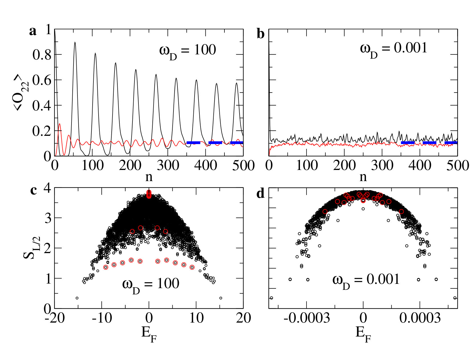 Figure 1
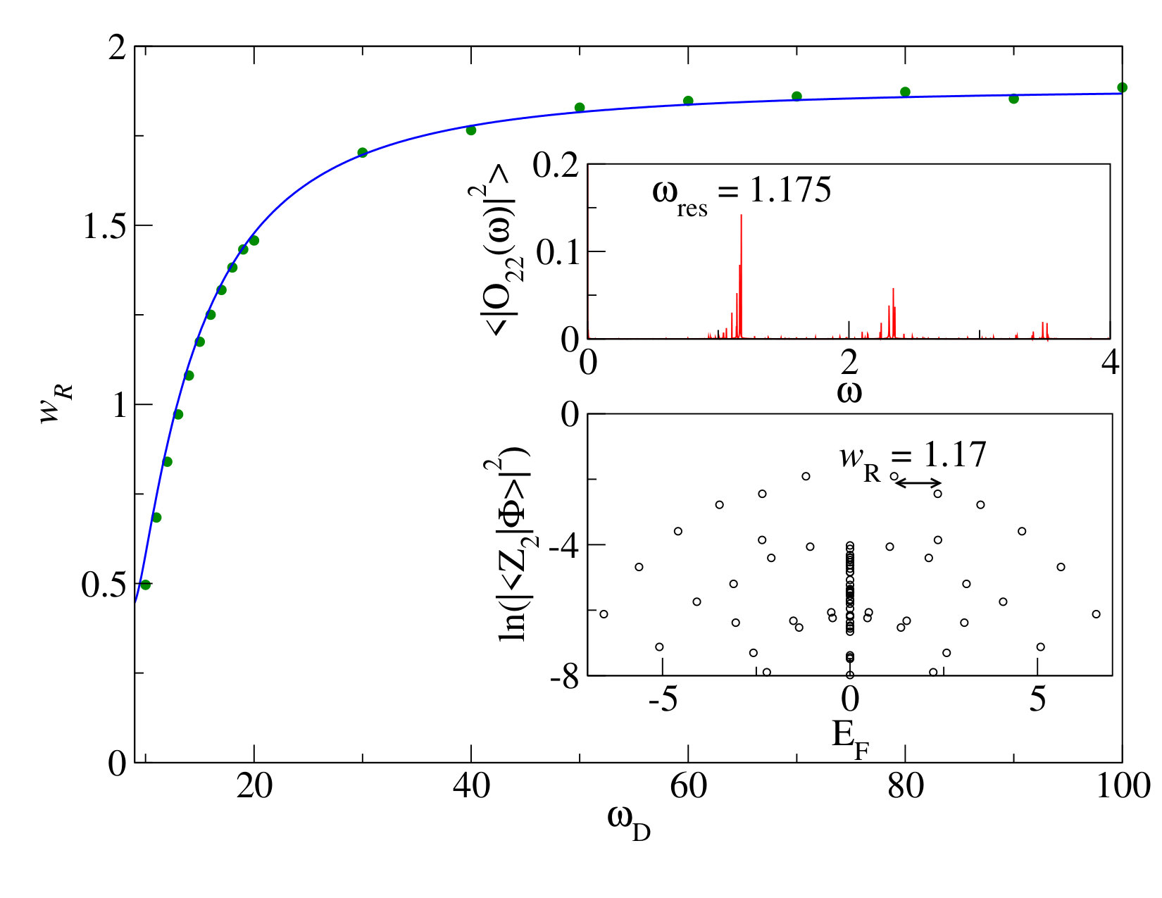 Figure 2
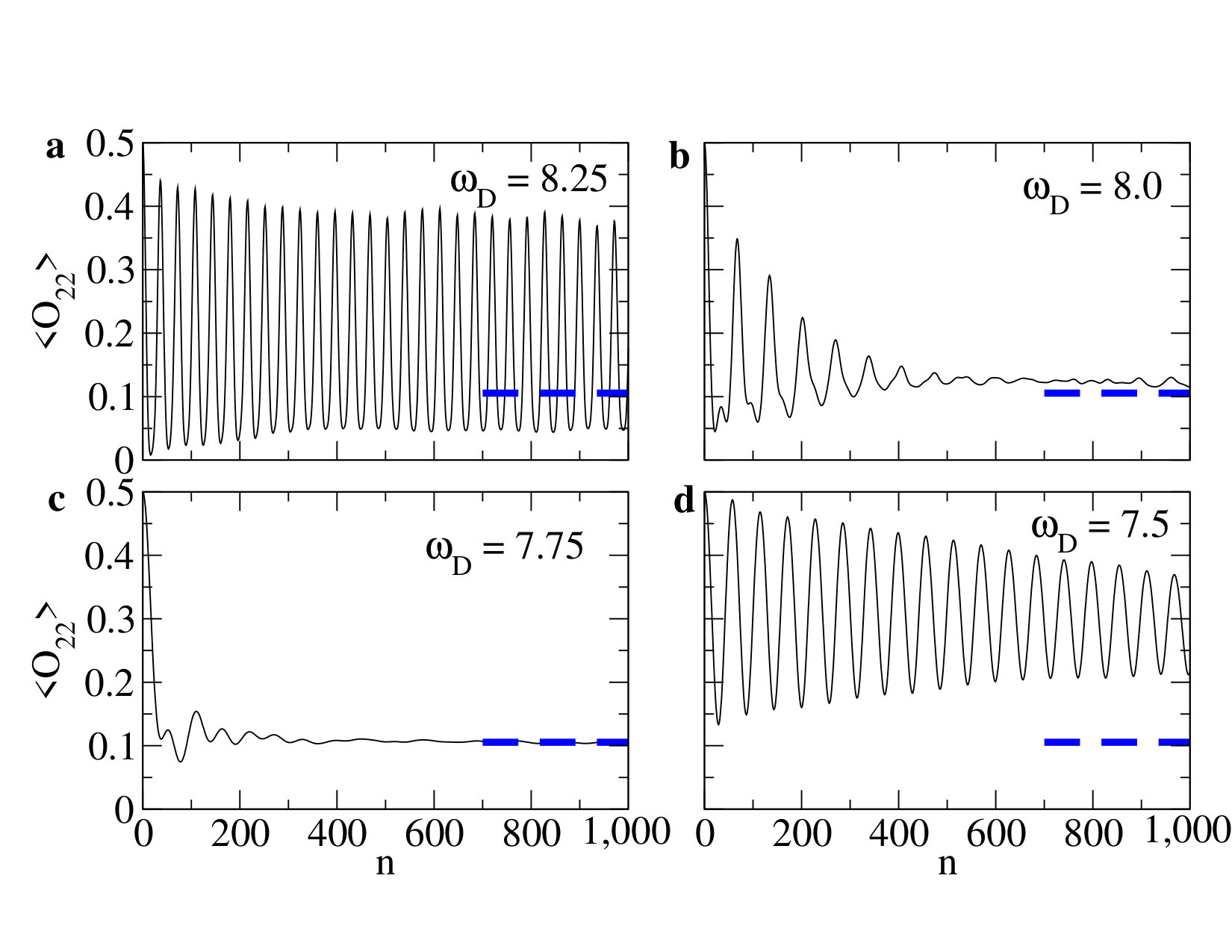 Figure 3
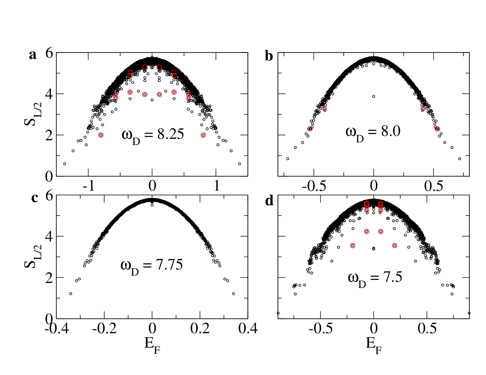 Figure 4
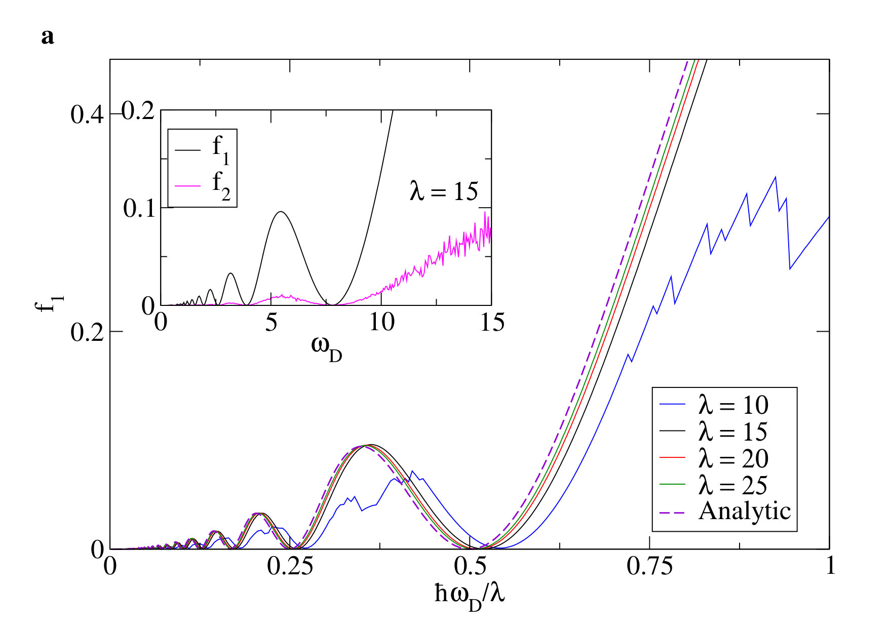 Figure 5
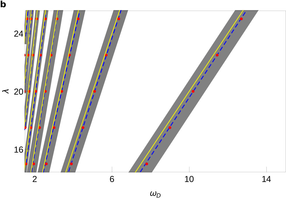 Figure 6
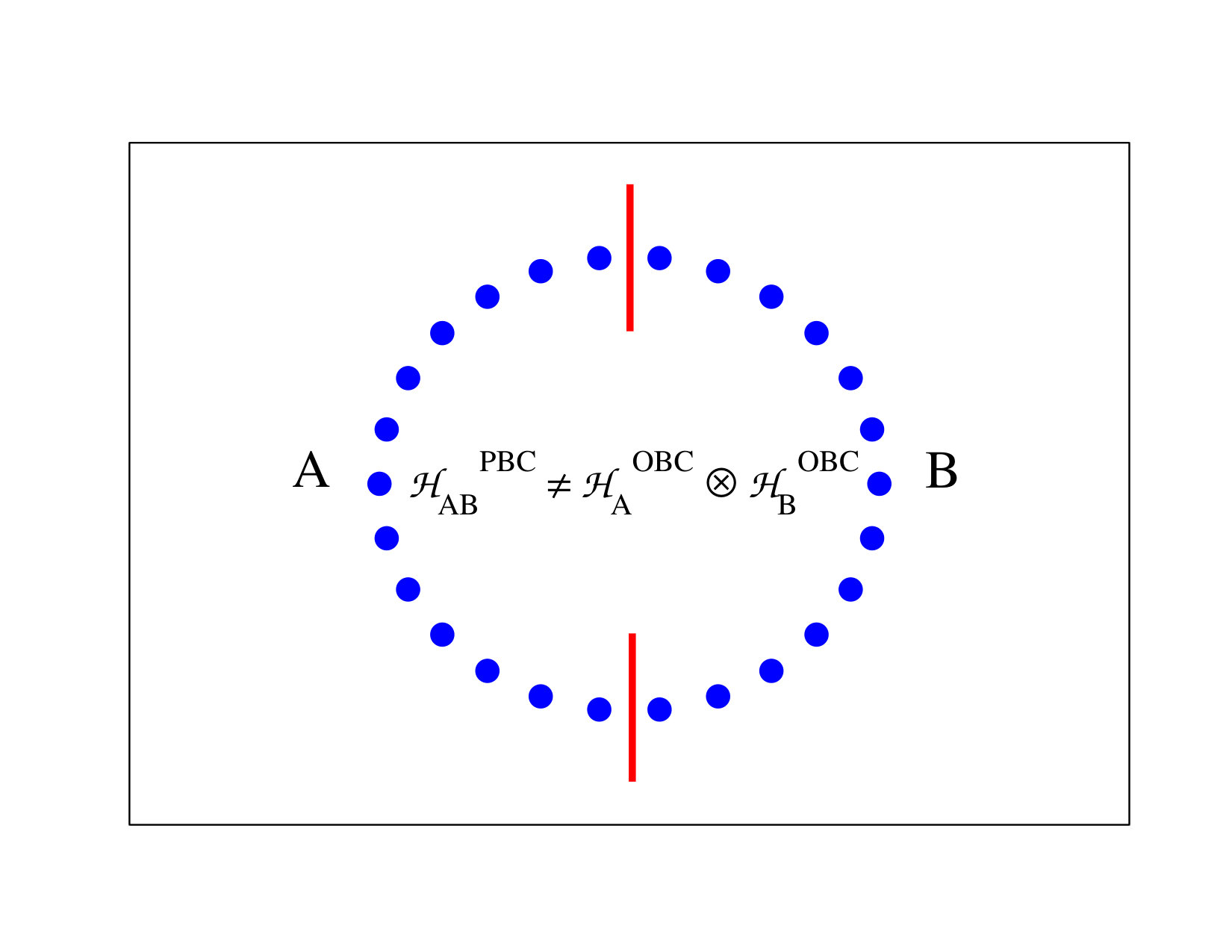 Figure 7
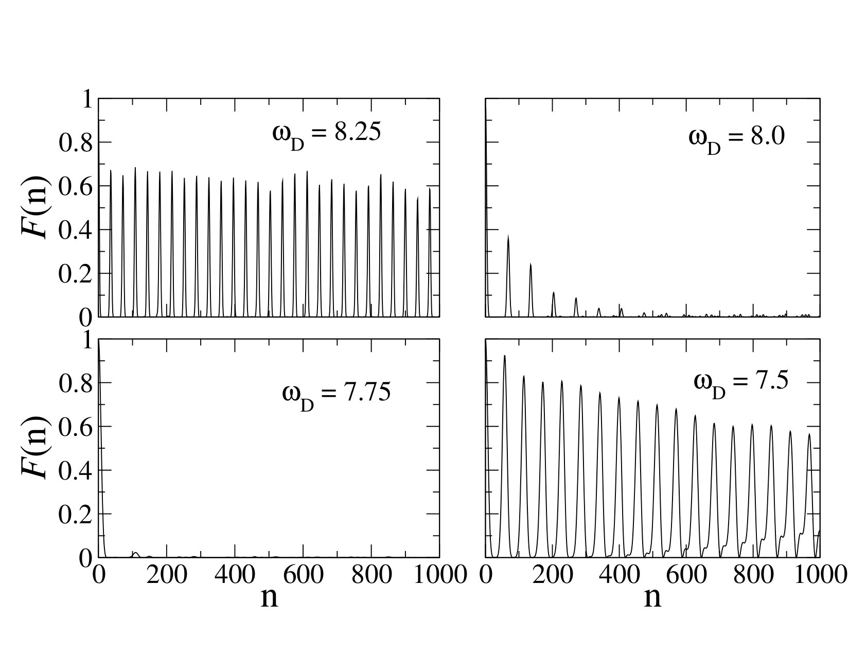 Figure 8
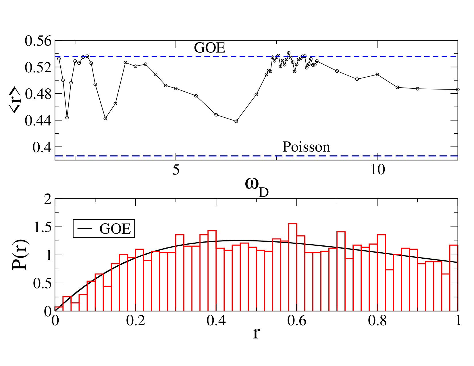 Figure 9
Peer Reviews
No public reviews on file for this paper yet. If you reviewed it on a platform where reviews are public (OpenReview, ICLR, NeurIPS, ICML), you can paste yours below so the community can read it here.
Videos
No videos yet. Explain this paper in a talk, walkthrough, or lecture? Add one.
Collapse and revival of quantum scars via Floquet engineering
Bhaskar Mukherjee1, Sourav Nandy1, Arnab Sen1, Diptiman Sen2, and K. Sengupta1
1School of Physical Sciences, Indian Association for the Cultivation of Science, Kolkata 700032, India
2Centre for High Energy Physics and Department of Physics, Indian Institute of Science, Bengaluru 560012, India
Abstract
The presence of quantum scars, athermal eigenstates of a many-body Hamiltonian with finite energy density, leads to absence of ergodicity and long-time coherent dynamics in closed quantum systems starting from simple initial states. Such non-ergodic coherent dynamics, where the system does not explore its entire phase space, has been experimentally observed in a chain of ultracold Rydberg atoms. We show, via study of a periodically driven Rydberg chain, that the drive frequency acts as a tuning parameter for several reentrant transitions between ergodic and non-ergodic regimes. The former regime shows rapid thermalization of correlation functions and absence of scars in the spectrum of the system’s Floquet Hamiltonian. The latter regime, in contrast, has scars in its Floquet spectrum which control the long-time coherent dynamics of correlation functions. Our results open a new possibility of drive frequency-induced tuning between ergodic and non-ergodic dynamics in experimentally realizable disorder-free quantum many-body systems.
The eigenstate thermalization hypothesis (ETH) is one of the central paradigms for understanding out-of-equilibrium dynamics of closed non-integrable quantum systems rev1a ; rev1b ; rev1c ; rev1d ; rev2 ; deutsch1 ; srednicki1 ; rigol1 . It posits that all bulk eigenstates of a generic quantum many-body Hamiltonian are thermal; their presence ensures ergodicity and leads to eventual thermalization for out-of-equilibrium dynamics of a generic many-body state rev2 . This hypothesis is strongly violated in certain cases, the most famous example being one-dimensional (1D) disordered electrons in their many-body localized phase mblref1 ; mblref2 . More recently another example of a weaker failure of ETH, due to the presence of quantum many-body scar states, has been studied extensively in disorder-free systems scarrefqm1 ; scarref1 ; scarref2a ; scarref2b ; scarref2c ; scarref2d ; scarref2e ; scarref3a ; scarref3b ; scarref3c ; scarref3d ; scarref3e . Scars are eigenstates with finite energy density but anomalously low entanglement scarref1 ; scarref2b ; scarref2c ; scarref2d ; scarref3b which form an almost closed subspace in the system’s Hilbert space under the action of its Hamiltonian. Their presence leads to persistent coherent oscillatory dynamics of correlation functions starting from initial states that have a high overlap with scars. This provides an observable consequence of their presence as verified in recent experiments on quench dynamics of a chain of ultracold Rydberg atoms scarref1 .
Here we study the fate of such ergodicity violation in a periodically driven Rydberg chain. It is well known that the stroboscopic dynamics of a periodically driven quantum system is controlled by its Floquet Hamiltonian rev3 which is related to its unitary evolution operator through , where is the time period of the drive and is the drive frequency. For generic disorder-free systems, such driving is expected to cause thermalization to a featureless “infinite temperature” state steady1b ; steady1c ; steady2 ; steady3 . In what follows, we will study the possibility of the existence of scars in the eigenstates of as a function of and relate their influence on the dynamics of correlation functions. Our initial state will be an experimentally realized symmetry broken many-body state which has one Rydberg excitation in alternate lattice sites scarref1 ; rydramp1 ; rydramp2 ; rydramp3 .
The central results of this study are as follows. First, for large and starting from a initial state, we show the presence of long-time persistent oscillations of the density-density correlator of Rydberg atoms. Such oscillations have characteristic frequencies which are different from indicating a lack of synchronization (a hallmark of thermalization in periodically driven systems). We relate this oscillation frequency to the quasienergy separation between the scar states of the Floquet Hamiltonian indicating the central role of these states in the dynamics. Second, at ultra-low drive frequencies, we find that there are no persistent oscillations, and the behavior of the correlator agrees with that expected from ETH. We show numerically that in this regime, there are no scars in the eigenspectrum of and the dynamics is controlled by a set of thermal states. Finally, we find several drive-frequency-induced transitions between thermal and coherent regimes at intermediate frequencies. These transitions, that have no analogs in the non-driven systems studied earlier scarref1 ; scarref2a ; scarref2b ; scarref2c ; scarref2d ; scarref2e ; scarref3a ; scarref3b ; scarref3c ; scarref3d ; scarref3e , provide a route to controlled switching between ergodic and non-ergodic dynamics of the Rydberg atoms. We chart out the critical drive frequencies at which these transitions occur, provide an analytic understanding of their occurrence, and suggest experiments which can test our theory.
Model: The low-energy properties of an ultracold Rydberg atom chain can be described by an effective two-state Hamiltonian on each site given by scarref1 ; rydramp1 ; rydramp2 ; rydramp3
[TABLE]
The two states correspond to the ground () and Rydberg excited states () of the atoms on site . The dipole blockade in these systems ensures that there is at most one Rydberg excitation per site: , where is the Rydberg excitation number operator, and denotes a Pauli matrix on site which couples the ground and excited states. In Eq. (1), is the detuning parameter which can be used to excite an atom to its Rydberg state, denotes an interaction between two Rydberg excitations, and is the coupling strength between ground and excited states. In experiments, it is possible to reach a regime where so that the Hamiltonian of the model becomes scarref1 ; dipoleexp1 ; dipoleexp2 ; subir1 ; subir2
[TABLE]
and this is to be supplemented by the constraint that for all sites .
This constrained model can be easily mapped into an Ising-like spin model in the presence of both longitudinal and transverse fields of strength and respectively. Within the constrained Hilbert space of the system, one can represent as scarref2c ; scarref2d
[TABLE]
where is a local projection operator, and , , and . Our analysis will be based on this model. Eq. (3) also provides a low-energy description for the 1D tilted Bose-Hubbard model as detailed in the Supplementary Information. For , reduces to the “PXP model” studied in Refs. scarref2c ; scarref2d which is known to host quantum scars among its eigenstates.
Analysis: We analyze the periodic dynamics of for a square pulse protocol: for . The unitary evolution operator at the end of a drive cycle can be written as . The evolution operator can then be expressed as
[TABLE]
where and are eigenstates and eigenfunctions of and . The spin correlation function of the spins between any two sites and can then be obtained, after drive cycles, as
[TABLE]
where for , and is the initial state. Unless explicitly stated otherwise, we will choose to be a symmetry broken state, with . We note that provides direct information of the density-density correlation function of the Rydberg atoms after cycles of the drive. Our numerical analysis will involve computation of and using exact diagonalization for finite chains of size and subsequent evaluation of using Eq. (5).
To obtain an analytical understanding of the nature of the dynamics, we derive the Floquet Hamiltonian corresponding to using a Magnus expansion which is expected to yield an accurate description of the dynamics for high drive frequencies rev3 . Further details are provided in Supplementary Information. To , this calculation leads to , where
[TABLE]
Here we have defined dimensionless quantities and , , and . We find that the terms in (which we denote as PXP terms) constitute a renormalized PXP model (up to a global spin rotation); consequently, for , where the effect of can be ignored, we expect to host scar states similar to those in the PXP model. However at moderate , the terms in (which we denote as non-PXP terms), are expected to become important. The competition between these two classes of terms can be tuned using the drive frequency and will be discussed in detail below.
In what follows, we will be interested in large drive amplitudes for which (). In this regime, as detailed in Supplementary Information, the Floquet Hamiltonian can be perturbatively calculated to for an arbitrary and gives only PXP terms with all non-PXP terms (and further PXP terms) generated at and beyond. To , the Floquet Hamiltonian equals
[TABLE]
Eq. (7) will be used to understand the transitions between ergodic and non-ergodic regimes.
Results: To demonstrate the presence of ergodic to non-ergodic transitions as a function of the drive frequency , we first compute the dynamics of the correlators starting from . For this, we perform exact diagonalization and compute from Eq. (5) as a function of the stroboscopic time (number of drive cycles) for several . In addition we also compute the half-chain entanglement entropy for the eigenstates of the Floquet spectrum by obtaining these via numerical diagonalization of (Eq. (4)). This is followed by a computation of the reduced density matrix for these eigenstates for a half chain from which can be obtained using a standard procedure (see Supplementary Information). Quantum scars have and are thus expected to have much lower entanglement compared to thermal states for which . Thus provides a reliable way to distinguish between thermal states and scars for a finite-size many-body system.
The results of these calculations are shown in Fig. 1. Panel a [b] of Fig. 1 shows the behavior of as a function of for . We find that for , the dynamics exhibits long-time coherent oscillations as expected from the quench dynamics of the PXP model at studied earlier scarref2c ; scarref2d . The frequency of these oscillations differs from indicating a clear lack of synchronization. This behavior is expected from Eq. (6) where the non-PXP terms appear in and hence are small. The presence of scars in the Floquet Hamiltonian in this regime may be confirmed from Fig. 1 (c)which shows for Floquet eigenstates (denoted by henceforth) as a function of the Floquet quasienergies . The scar states are seen as clear outliers in this plot. The eigenstates with large overlaps with () are circled in red; from this we find that the scars have maximal overlap with and thus control the dynamics leading to violation of ETH scarref2d .
In contrast, for , all the states including those controlling the dynamics are thermal (Fig. 1 (d)). Consequently, there are no persistent oscillations for (Fig. 1 (b)) and one finds thermalization consistent with ETH. We also note that the oscillatory behavior seen in Fig. 1 is a property of the initial state; a similar study of the dynamics for any drive frequency starting from the Rydberg vacuum state always provides fast thermalization consistent with ETH (red curves in Fig. 1 (a) and (b)).
The quasienergy separation of the scars for as a function of is shown in Fig. 2. We note that starts to decrease when ; such a behavior follows from the decrease of the norm of the PXP terms in at with increasing (Eq. (7)) which gives , where is the scar quasienergy separation for the undriven PXP model. Fig. 2 shows the exact match of the numerical result with that obtained analytically. The lowering of implies a sharp decrease in the oscillation frequency of as a function of in this regime. To check this, we extract as a function of from the Fourier transform of (upper inset of Fig. 2) which matches the corresponding values of almost perfectly (lower inset of Fig. 2) and shows a clear decrease with . This provides a drive-induced control over the quasienergy separation of the scars and hence on the oscillation frequency which has no analog in earlier quench studies. (Interestingly, the bottom inset of Fig. 2 shows a large number of states with zero quasienergy. They arise due to a symmetry of the Floquet operator as discussed in Supplementary Information).
Next, we analyze the regime where we encounter the reentrant transitions between coherent and thermal regimes. Here, we follow Ref. scarref2c ; scarref2d and use the state as our initial state, where denotes the spin-flipped version of . This allows us access to larger chain length since has weight only in the sector with zero total momentum and spatial inversion (parity) symmetry.
The result of evolution of in this subspace is shown in Fig. 4 near the first reentrant transition. Fig. 4 (a) shows non-ergodic persistent oscillatory dynamics at . As we reduce , these oscillations dampen (Fig. 3 (b)); such a behavior can be interpreted as a precursor to ergodic dynamics and thermalization. Upon further reduction of , ergodic dynamics consistent with ETH sets in and the fastest thermalization is seen around (Fig. 3 (c)). Finally, at lower , the persistent oscillations return (Fig. 3 (d)).
Such transitions between non-ergodic and ergodic dynamics as a function of drive frequency can be tied to the presence or absence of scars in the spectrum of . This is shown in Fig. 4. Figs. 4 (a)() and (d) () clearly indicate the presence of scars having high overlap with . This is consistent with the presence of non-ergodic dynamics characterized by persistent long-time oscillations (Figs. 3 (a, d)). These scar states start to merge with the thermal band around (Fig. 4 (b)) indicating precursor to the thermal behavior (Fig. 3 (b)). Fig. 4 (c) at shows complete absence of scars resulting in ergodic dynamics of and fast thermalization predicted by ETH (Fig. 3 (c)).
To obtain a qualitative understanding of these transitions, we compute the norm of the PXP-like terms in the Floquet Hamiltonian numerically using . To this end, we write the matrix representation of in the basis states of and identify the matrix elements that have . Let us denote this set as which has elements (where is a Fibonacci number defined by with ). We then define and as
[TABLE]
Clearly, represents the contribution from the non-PXP type of terms in . We note that in general will also have contributions from non-PXP terms since such terms may have non-zero matrix elements for some states included in . However, at large , the contributions from these terms are expected to be small by at least . In fact from Eq. (7), to leading order, we find that
[TABLE]
To numerically verify that this is indeed the case, we plot as a function of for several (Fig. 5 (a)). These curves coincide indicating that is almost independent of . Thus in this regime receives negligible contributions from the non-PXP terms in which necessarily depend on (Fig. 5 (a) also shows that lies outside this regime).
Fig. 5 (a) and Eq. (9) also show that is an oscillatory function of . From the inset of Fig. 5 (a), we find that near the minima of at (Eq. (9)) where is a positive integer; in other regions, . The ergodic dynamics of always occur in a finite frequency interval around (where ). This observation sheds light on the cause of the transitions. We note that the PXP Hamiltonian supports scars; consequently, for where is PXP-like (), one expects the presence of scars among its eigenstates. These scars lead to coherent non-ergodic dynamics. In contrast, near the minima of , where , receives significant contributions from the non-PXP terms. In the presence of such terms which can be long-ranged at low , does not support scars. The bulk of its eigenstates around are thermal; consequently the dynamics of displays ergodic behavior consistent with the prediction of ETH. In fact, the level spacing statistics of the eigenvalues of follow a Gaussian orthogonal ensemble for as expected for an ergodic system (see Supplementary Information). The behavior of the fidelity , where is the state after drive cycles, across the transition is also discussed in the Supplementary Information.
The schematic phase diagram for these reentrant ergodic to non-ergodic transitions is summarized in Fig. 5 (b). The ergodic regions, where displays either complete ergodic behavior or a precursor to thermalization, are located in a small frequency window (shown schematically in grey) around (indicated as red dots joined by blue dashed lines in Fig. 5 (b)). The yellow lines indicate the positions of the transitions as obtained from Eq. (7) (i.e., is an even integer), while the white regions denote the ranges of where shows non-ergodic oscillatory dynamics due to the presence of scars in . The thermal regions become denser with decreasing and ultimately merge into a continuum at sufficiently small where non-ergodic coherent dynamics of ceases to exist.
Discussion: To summarize, we have studied the kinematically constrained PXP model, a paradigmatic model for many-body eigenstates called quantum scars that violate ETH, in the presence of a pulsed transverse magnetic field that varies periodically in time. In the limit of large drive amplitude of the field, the instantaneous Hamiltonian does not have any scars but the corresponding Floquet Hamiltonian that controls the stroboscopic dynamics of local quantities can still host them depending on the drive frequency. We find (a) the presence of several non-ergodic (characterized by a coherent oscillatory behavior of density-density correlators and scars in the Floquet Hamiltonian) and ergodic (characterized by a thermal non-oscillatory behavior of density-density correlators and absence of scars) regimes as a function of the driving frequency, and (b) the possibility of tuning the quasienergy spacing of the scars in the non-ergodic regime as a function of the drive frequency to control the frequency of oscillations of the correlators. Both these features are entirely absent in the undriven PXP model and can be tested by standard experiments using finite-size Ryberg chains and starting from an initial state that has one Rydberg excitation at each alternate lattice site. In particular, these reentrant transitions from non-ergodic to ergodic regimes by tuning the drive frequency are possibly the first example of this kind in a system without any spatial disorder.
The mechanism for these transitions is also rather transparent in the large drive amplitude regime as discussed here. Using a Floquet perturbation theory, the Floquet Hamiltonian can be grouped into PXP and non-PXP type terms, with the non-PXP terms being suppressed by at least the inverse of the drive amplitude. The leading PXP terms can be resummed to all orders in the drive frequency which shows that these can diminish and become comparable to the non-PXP terms in the neighborhood of special drive frequencies leading to the emergence of the thermal regime. Lastly, on a theoretical front, it would be interesting to explore the influence of the small non-PXP terms in the non-ergodic regime to see whether they lead to eventual thermalization on a much longer time scale.
Acknowledgments: The work of A.S. is partly supported through the Max Planck Partner Group program between the Indian Association for the Cultivation of Science (Kolkata) and the Max Planck Institute for the Physics of Complex Systems (Dresden). D.S. thanks DST, India for Project No. SR/S2/JCB-44/2010 for financial support.
I Supplementary Material
II Model Hamiltonian
The Hamiltonian of the Bose-Hubbard model with a tilt is given by subir1
[TABLE]
where () denotes the boson annihilation (creation) operator on site of a 1D chain, is the boson number operator, is the hopping amplitude of the bosons, denotes the magnitude of the tilt, is the chemical potential, is the hopping amplitude, and is the on-site interaction between the bosons. The tilt can be generated either by shifting the center of the parabolic trap confining the bosons or by applying a linearly varying Zeeman field which couples to the spin of the bosons. The latter variation can be made time dependent by using a magnetic field which varies periodically in time. It is well known that the low-energy physics of these bosons deep inside the Mott phase, whose occupation number is denoted by , (here we focus on the case ) and where , is given by
[TABLE]
where denotes a dipole annihilation operator on link between sites neighboring and on a 1D lattice, for , is the dipole number operator on link , is the amplitude of spontaneous dipole creation or destruction, and is the chemical potential for the dipoles. This dipole model is to be supplemented by two constraints which make it non-integrable: and for all links. The phase diagram of this model has been studied theoretically in Ref. subir1, and has also been experimentally verified dipoleexp1 . It is well-known that support a quantum phase transition at separating a symmetry broken ground state () for and a featureless dipole vacuum () for . The non-equilibrium dynamics of this model has also been studied for quench, ramp and periodic protocols dipoledyn .
The dipole model described in Eq. (S2) also serves as an effective model for describing the low energy physics of the Rydberg atoms. To see this we first consider the Hamiltonian of such atoms given by scarref1 ; scarref1p5 ; scarref2 ; scarref3 ; rydramp
[TABLE]
Here denotes the number of Rydberg excitations on a given site, is the detuning parameter which can be used to excite an atom to its Rydberg state, denotes the interaction between two Rydberg excitations, denotes the coupling between the ground () and Rydberg excited () states, and is the corresponding coupling strength. In experiments scarref1 , it is possible to reach a regime where ; in this case, the Hamiltonian the model becomes equivalent to that of
[TABLE]
supplemented by the constraint that for all sites . Clearly, this model is equivalent to Eq. (S2) with the identification , and .
Furthermore it is also easy to see that the dipole Hamiltonian (Eq. (S2)) is identical to the PXP model studied in Ref. scarref1, for . The simplest way to see this involves mapping of the dipole operators to Ising spins via the transformation
[TABLE]
where denote the Pauli matrices for . Moreover, the constraint of not having dipoles on adjacent links can be implemented via a local projection operator scarref1p5 ; scarref2 . Using these, one finds the spin Hamiltonian
[TABLE]
where for , and we have ignored an unimportant constant term while writing down the expression for . The physics of within the constrained dipole Hilbert space is identical to that of and . At , reduced to the PXP model studied in Ref. scarref1, . Note that both the constraints of the dipole model are incorporated in via the local projection operators .
Eq. (S6) has been used for the analysis in the main text.
III Magnus expansion
We consider the Hamiltonian given by Eq. (S6) in the presence of a periodic drive characterized by a square pulse protocol with time period , where is the drive frequency: for . In what follows, we will chart out the details of the computation of the Floquet Hamiltonian of such a driven system using a high-frequency Magnus expansion.
For this protocol, the unitary matrix governing the evolution by a time period is given by
[TABLE]
where . For future reference, we also define given by
[TABLE]
such that . The Floquet Hamiltonian can be obtained from as . Using the Baker-Campbell-Hausdorff formula, one can express
[TABLE]
From Eq. (S9) we can find terms of different order in the Floquet Hamiltonian. The computation of these terms up to is straightforward and yields
[TABLE]
where . Note that these terms lead to a renormalized PXP model; it amounts to a change of magnitude of the coefficient of the standard PXP Hamiltonian and also a rotation in spin-space which depends on . Note that the second order term in the expansion has an opposite sign compared to the zeroth order term. As we will see later, this is a general feature of the model; any term in the renormalized PXP model always comes with a opposite sign compared to a term .
The first non-trivial longer-ranged terms in arises in . Its derivation involves some subtle issues. To see this, let us consider the commutator . It is easy to see after a straightforward calculation that
[TABLE]
We note that within the constrained Hilbert space, any term with identically vanishes for . Furthermore, the projection operators on any link satisfy for . Using these results, we can simplify to obtain
[TABLE]
Using Eq. (S12) and evaluating the necessary commutators, we finally get , where
[TABLE]
Here , and we note that in the limit of large . Thus Eqs. (S10) and (S13) yield in the main text while Eqs. (S14 - S16) yield . This completes our derivation of the Magnus expansion to .
Before ending this section we note that if we concentrate on the large limit, it is possible to compute higher-order corrections to the coefficients in and . This can be seen by noting that at each order the contribution to such terms comes from , i.e., the -th order contribution involves commutator of terms involving and one . These commutators provide the leading contribution in the large limit. This structure allows us to compute leading higher-order terms in the Magnus expansion which contribute to the coefficients of the PXP term. A straightforward but cumbersome computation yields
[TABLE]
It will be shown in Sec. IV that the coefficients in can be resummed to yield a closed form valid for arbitrary : .
IV Floquet perturbation theory
We will now present a perturbation theory for a periodically driven system soori . We consider a Hamiltonian , where varies in time with a period , and is a small time-independent perturbation. We will assume that commutes with itself at different times, and will work in the basis of eigenstates of which are time-independent and will be denoted as , so that , and . We will also assume that is completely off-diagonal in this basis, namely, for all . We will now find solutions of the Schrödinger equation
[TABLE]
which satisfy
[TABLE]
For , we have , so that the eigenvalue of the Floquet operator is given by
[TABLE]
We will now develop a perturbation theory to first order in . We assume that the -th eigenstate can be written as
[TABLE]
where for all , while is of order for all and all . Eq. (S18) implies that
[TABLE]
where the dot over denotes . Taking the inner product of Eq. (S22) with and using , we find that . We can therefore choose for all . We thus have
[TABLE]
Hence Eq. (S19) implies that the Floquet eigenvalue is still given by Eq. (S20) up to first order in .
Next, taking the inner product of Eq. (S22) with , where , and integrating from to , we get
[TABLE]
Since we know that Eq. (S23) satisfies
[TABLE]
we must have
[TABLE]
for all . Eqs. (S24-S26) imply that we must choose
[TABLE]
We see that is indeed of order provided that the denominator on the right hand side of Eq. (S27) does not vanish; we will call this case non-degenerate.
The above analysis breaks down if
[TABLE]
for a pair of states and . We then have to develop a degenerate perturbation theory. Suppose that there are states () which have energy eigenvalues satisfying Eq. (S28) for every pair of states. Ignoring all the other states of the system for the moment, we will assume that a solution of the Schrödinger equation is given by
[TABLE]
where we now allow all the ’s to be order 1. Then we again obtain an equation like Eq. (S22) except that the sum over only goes over states. To first order in , we can replace by the time-independent constants on the right hand side of Eq. (S22). Upon integrating from to , this gives
[TABLE]
This can be written as a matrix equation
[TABLE]
where denotes the column (where the superscript denotes transpose), is the -dimensional identity matrix, and is a -dimensional Hermitian matrix with matrix elements given by
[TABLE]
Let the eigenvalues of be given by (). To first order in , is a unitary matrix and will therefore have eigenvalues of the form ; the corresponding eigenstates satisfy . Next, we want the wave function in Eq. (S29) to satisfy . This implies that the Floquet eigenvalues are related to the eigenvalues of as
[TABLE]
Given a Floquet operator , we can define a Floquet Hamiltonian as . Comparing this with Eqs. (S31) and (S32), we see that the matrix elements of are given by
[TABLE]
We will now apply the above analysis to our model, where
[TABLE]
with for and for . We will do Floquet perturbation theory assuming that . To do this, we consider states in the basis. According to the Hamiltonian in Eq. (S35), all such states have an instantaneous energy eigenvalue , which implies that the . Thus the unperturbed Floquet eigenvalue is equal to 1 for all states; we therefore have to do degenerate perturbation theory.
If and are two states which are connected by the perturbation in Eq. (S35), they differ by the value of at only one site and therefore , assuming that and have spin-up and spin-down respectively at that site. We find that the integral in Eq. (S30) is given by
[TABLE]
We therefore see that if
[TABLE]
where is an integer, then the expression in Eq. (S36) vanishes. This means that even in degenerate perturbation theory, there is no change in the Floquet eigenvalues and they remain equal to 1.
We will now use Eqs. (S34) and (S36). If and are two states which are connected by the perturbation , we have . We then obtain
[TABLE]
where . The Floquet Hamiltonian is therefore given by
[TABLE]
This vanishes if Eq. (S37) is satisfied; we will then have to go to higher order in perturbation theory.
We note that Eq. (S39) can also be obtained by a straightforward expansion of the evolution operators . To see this, we first note that for any two different sites and we have
[TABLE]
Thus as long as we are interested in terms of , we can write
[TABLE]
One can then carry out a straightforward expansion of . A few lines of algebra, required to gather terms of , yield
[TABLE]
Using Eq. (S42), one can compute . A re-exponentiation of terms of then yields Eq. (S39) in a straightforward manner.
Next, we note that the magnitude of the right hand side of Eq. (S38) is independent of and . Hence
[TABLE]
where the sum runs over all all pairs of states which are connected by .
Given a system of size and periodic boundary condition (), and the constraint that two up-spins cannot be on neighboring sites in any state, we can find the number of states and the value of in Eq. (S43). To this end, we first define the Fibonacci numbers which satisfy , with ; as increases, quickly approaches , where is the golden ratio. Keeping the up-spin constraint in mind, we define the transfer matrix
[TABLE]
where the indices of can take values 1 (spin-up) and 2 (spin-down). The number of states in an -site system is then given by . To calculate , we note that a spin at, say, site 2, can flip between up and down only if the spins at sites 1 and 3 are both down. The contribution of all such states to is 2 times the number of all possible states for sites 4 to with open boundary condition () and the up-spin constraint; the factor of 2 is because the spin at site 2 can be up or down, giving two states. Since the number of bonds for an system with sites 4 to is , the number of states for such a system is given by the sum of all the matrix elements of . This is equal to . In the above argument, we assumed that there the spin which can flip between up and down is at site 2. However, the site 2 could have been anywhere else in the -site system. We therefore see that . This leads us to define the normalized quantity
[TABLE]
V Symmetry of Floquet operator and zero modes
We will now discuss an exact symmetry of the Floquet operator for our driving protocal. We will then see that this symmetry implies that there will be a large number of states with zero quasienergy.
We define an operator
[TABLE]
which is unitary and satisfies . The eigenvalues of are , and the corresponding eigenstates have an even (odd) number of down spins. Next, we see that anticommutes with the first term and commutes with the second term in Eq. (S6). As a result, the Floquet operator defined in Eq. (S7) satisfies
[TABLE]
This means that if is an eigenstate of with eigenvalue , will be an eigenstate of with eigenvalue . Hence, all the quasienergies must come in pairs, except for quasienergies 0 and which correspond to Floquet eigenvalues equal to . We also see that eigenstates of with eigenvalues can be simultaneously chosen to be eigenstates of ; hence they will be superpositions of states all of which have an even or an odd number of down spins.
Given the Floquet Hamiltonian defined through , Eq. (S47) implies that
[TABLE]
Note that this is an exact symmetry, independent of the Magnus expansion or Floquet perturbation theory. We will now use the arguments given in Ref. scarref1p5, to argue that there will be a large number of eigenstates of with zero eigenvalue; we will call these zero modes. Eq. (S48) implies that can be thought of as defining a tight-binding model of a particle moving on a bipartite lattice, where the two sublattices correspond to eigenvalues of being equal to . For such a tight-binding model, it is known that a lower bound on the number of zero modes is given by the difference of the number of states with equal to .
Next, we use the parity symmetry of our system corresponding to a reflection about the middle of the bond connecting sites labeled and (we will assume that is even). We define a parity transformation which does this reflection. Given an arbitrary state , the parity transformed state is . The superpositions then give two states with even (odd) parity respectively. However, states of the product form
[TABLE]
where each can be spin-up or down, clearly satisfy . Such states therefore lie in the even parity sector; further, they have eigenvalue of equal to since each value of appears twice in Eq. (S49). Let the number of such states be (we will calculate this number below). Now, let denote the number of orthonormal states with (denoting even/odd) and (denoting ). We then see that and . A lower bound on the number of zero modes in the odd parity sector is , and in the even parity sector is . Since
[TABLE]
regardless of the values of and , we see that gives a lower bound on the number of zero modes.
To calculate the number , we note that the string for the first sites in Eq. (S49) must begin and end with a down spin to ensure that the neighboring sites and do not both have spin-up. The number of of such strings is given by the matrix element of ; this gives . Thus the number of zero modes increases exponentially with , as .
VI Half-chain entanglement
Here we detail out the procedure for computation of the half-chain entanglement used in the main text. The procedure could be applied to equilibrium or Floquet eigenstates or to an arbitrary driven state of the given model in Eq. S6.
We first note that the full density matrix () is given by where is the whole system of size with . We divide this system into two parts and of size each with as schematically shown in Fig. S1.
Next, we calculate the reduced density matrix of any of the subsystems by integrating out the other subsystem. This leads to
[TABLE]
This procedure involves taking a partial trace over the environment degrees of freedom. For example, the -th element, , of the reduced density matrix is given by
[TABLE]
where and represent product states in , and represent product states in with OBC. However, since the full system () had PBC, the Hilbert space dimension (HSD) of does not match the HSD of with OBC. To see this, we note that and , where denotes the -th Fibonacci number. Since for any , one has for any . Thus, while taking the summation in Eq. (S51), one has to exclude the states for which at any one of the junctions marked in red in Fig. S1, the end points of both and are occupied by a dipole.
Since the Hamiltonian and hence the full density matrix is in the configuration (product) basis, any matrix element of the reduced density matrix can be expressed as a sum of some of the elements of full DM, and we can rewrite Eq. (S52) as
[TABLE]
We stress here that one needs to be careful about this procedure if the density matrix is expressed using some other basis. For example in our case where , are states in the zero total momentum () and even parity () sector. In this case
[TABLE]
This indicates that one needs to search for states , having non-zero overlap with the states and given by
[TABLE]
In this case, -th element of is given by
[TABLE]
and the diagonalization of gives the Von-Neumann entropy since , where are the eigenvalues of . This procedure is used to compute in the main text.
VII Fidelity and Level statistics
In this section, we note that the transitions from the ergodic to non-ergodic behaviors will also manifest themselves in the fidelity and eigenvalue statistics.
The fidelity of the driven Rydberg chain computed after cycles of the drive is defined as
[TABLE]
where denotes the state of the system after cycles of the drive, and is the initial state. In the regime where the dynamics is dominated by scars, the presence of long-term coherent oscillations indicates that one could expect periodic revival of to values near unity; in contrast, the thermal region, is expected to decay rapidly to zero and never revive. These behaviors are numerically confirmed in Fig. S2 near the ergodic to non-ergodic transition around . The top left () and the bottom right () panels display periodic persistent revivals of before and after the first transition. Such revivals are completely absent in the bottom left panel () in the thermal region where decays to zero without any subsequent revival. The top right panel () shows an intermediate behavior displaying a few (smaller) revivals and subsequent decay. This indicates a crossover from a coherent to a thermal regime.
Next we discuss the characteristics of eigenvalue statistics across the transition. To this end, we first arrange the Floquet eigenvalues () (excluding the zero modes) in ascending order in the range , and then calculate the gaps between adjacent eigenvalues. This allows us to compute the distribution of the ratio of successive gaps in the energy spectrum huse
[TABLE]
The distribution of for an ergodic (thermal) system obeys the Gaussian orthogonal ensemble (GOE) and can be computed using random matrix theory Atas to be
[TABLE]
with an average value . In contrast, for a fully non-ergodic (localized) system, the distribution of is Poissonian with . In Fig. S3, we plot vs computed using the eigenvalues of . The plot indicates that reaches its GOE form precisely at the transition points; it remains lower than this value for other . It is to be noted that never reaches its Poisson value which indicates non-integrability of the system for all . This confirms the signature of the transition in the level statistics.
References
- (1) S. Sachdev, K. Sengupta, and S. M. Girvin, Phys. Rev. B 66, 075128 (2002); S. Pielawa, T. Kitagawa, E. Berg, and S. Sachdev, Phys. Rev. B 83, 205135 (2011).
- (2) J. Simon, W. S. Bakr, R. Ma, M. E. Tai, P. M. Preiss, and M. Greiner, Nature (London) 472, 307 (2011); W. Bakr, A. Peng, E. Tai, R. Ma, J. Simon, J. Gillen, S. Foelling, L. Pollet, and M. Greiner, Science 329, 547 (2010).
- (3) K. Sengupta, S. Powell, and S. Sachdev, Phys. Rev. A 69, 053616 (2004); M. Kolodrubetz, D. Pekker, B. K. Clark, and K. Sengupta, Phys. Rev. B 85, 100505 (2012); U. Divakaran and K. Sengupta, Phys. Rev. B 90, 184303 (2014).
- (4) H. Bernien, S. Schwartz, A. Keesling, H. Levine, A. Omran, H. Pichler, S. Choi, A. S. Zibrov, M. Endres, M. Greiner, V. Vuletic, and M. D. Lukin, Nature 551, 579 (2017).
- (5) C. J. Turner, A. A. Michailidis, D. A. Abanin, M. Serbyn, and Z. Papic, Nat. Phys. 14, 745 (2018); ibid, Phys. Rev. B 98, 155134 (2018).
- (6) S. Choi, C. J. Turner, H. Pichler, W. W Ho, A. A. Michailidis, Z. Papic, M. Serbyn, M. D. Lukin, and D. A. Abanin, Phys. Rev. Lett. 122, 220603 (2019); W. W. Ho, S. Choi, H. Pitchler, M. D. Lukin, Phys. Rev. Lett. 122, 040603 (2019); C. J. Turner, A. A. Michailidis, D. A. Abanin, M. Serbyn, and Z. Papic, arXiv:1905.08564 (unpublished); K. Bull, I. Martin, and Z. Papic, Phys. Rev. Lett. 123, 030601 (2019).
- (7) V. Khemani, C. R. Lauman, and A. Chandran, Phys. Rev. B 99, 161101 (2019); S. Maudgalya, N. Regnault, and B. A. Bernevig, Phys. Rev. B 98, 235156 (2018); ibid, arXiv:1906.05292 (unpublished); T. Iadecola, M. Schecter, and S. Xu, arXiv:1903.10517 (unpublished); N. Shiraishi, arXiv:1904.05182 (unpublished); M. Schecter and T. Iadecola, arXiv:1906.10131 (unpublished).
- (8) P. Fendley, K. Sengupta, and S. Sachdev, Phys. Rev. B 69, 075106 (2004); R. Samajdar, S. Choi, H. Pichler, M. D. Lukin, and S. Sachdev, Phys. Rev. A 98, 023614 (2018); R. Ghosh, A. Sen, and K. Sengupta, Phys. Rev. B 97, 014309 (2018).
- (9) A. Soori and D. Sen, Phys. Rev. B 82, 115432 (2010).
- (10) V. Oganesyan and D. A. Huse, Phys. Rev. B 75, 155111 (2007).
- (11) Y. Y. Atas, E. Bogomolny, O. Giraud, and G. Roux. Phys. Rev. Lett. 110, 084101 (2013).
The reference list from the paper itself. Each links out to its DOI / PubMed record.
- 1(1) Dziarmaga, J. Dynamics of a quantum phase transition and relaxation to a steady state. Adv. Phys. 59, 1063 (2010).
- 2(2) Polkovnikov, A., Sengupta, K., Silva, A. & Vengalattore, M. Colloquium: Nonequilibrium dynamics of closed interacting quantum systems. Rev. Mod. Phys. 83, 863 (2011).
- 3(3) Dutta, A., Aeppli, G., Chakrabarti, B. K., Divakaran, U., Rosenbaum, T. F. & Sen, D. Quantum Phase Transitions in Transverse Field Spin Models: From Statistical Physics to Quantum Information (Cambridge University Press, Cambridge, 2015).
- 4(4) Mondal, S., Sen, D. & Sengupta, K. Quantum Quenching, Annealing and Computation , edited by Das, A., Chandra, A. & Chakrabarti, B. K. Lecture Notes in Physics, Vol. 802 (Springer, Berlin, Heidelberg, 2010), Chap. 2, p. 21.
- 5(5) D’Alessio, L., Kafri, Y., Polkovnikov, A. & Rigol, M. From Quantum Chaos and Eigenstate Thermalization to Statistical Mechanics and Thermodynamics. Adv. Phys. 65, 239 (2016).
- 6(6) Deutsch, J. M. Quantum statistical mechanics in a closed system. Phys. Rev. A 43, 2046 (1991).
- 7(7) Srednicki, M. Chaos and quantum thermalization. Phys. Rev. E 50, 888 (1994); The approach to thermal equilibrium in quantized chaotic systems J. Phys. A 32, 1163 (1999).
- 8(8) Rigol, M., Dunjko, V. & Olshanii, M. Thermalization and its mechanism for generic isolated quantum systems. Nature (London) 452, 854 (2008).