Functional model for boundary-value problems
Kirill D. Cherednichenko, Alexander V. Kiselev, Luis O. Silva

TL;DR
This paper introduces a functional model for boundary-value problem operators, offering explicit resolvent formulas via Dirichlet-to-Neumann maps, aiding spectral and parameter-dependent analysis.
Contribution
It provides a novel functional model and explicit resolvent formulas for operators in boundary-value problems, enhancing spectral analysis capabilities.
Findings
Explicit resolvent formulas derived for boundary-value operators
Application of Dirichlet-to-Neumann maps in spectral analysis
Facilitation of parameter-dependent problem analysis
Abstract
We develop a functional model for operators arising in the study of boundary-value problems of materials science and mathematical physics. We then provide explicit formulae for the resolvents of the associated extensions of symmetric operators in terms of the associated generalised Dirichlet-to-Neumann maps, which can be utilised in the analysis of the properties of parameter-dependent problems as well as in the study of their spectra.
Click any figure to enlarge with its caption.
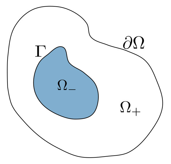 Figure 1
Peer Reviews
No public reviews on file for this paper yet. If you reviewed it on a platform where reviews are public (OpenReview, ICLR, NeurIPS, ICML), you can paste yours below so the community can read it here.
Videos
No videos yet. Explain this paper in a talk, walkthrough, or lecture? Add one.
\draftcopyName
DRAFT 130 \draftcopySetScale65
Functional model for boundary-value problems
Kirill D. Cherednichenko
Department of Mathematical Sciences, University of Bath, Claverton Down, Bath, BA2 7AY, United Kingdom
,
Alexander V. Kiselev
Departamento de Física Matemática, Instituto de Investigaciones en Matemáticas Aplicadas y en Sistemas, Universidad Nacional Autónoma de México, C.P. 04510, México D.F. and International Research Laboratory “Multiscale Model Reduction”, Ammosov North-Eastern Federal University, Yakutsk, Russia
and
Luis O. Silva
Departamento de Física Matemática, Instituto de Investigaciones en Matemáticas Aplicadas y en Sistemas, Universidad Nacional Autónoma de México, C.P. 04510, México D.F. and Department of Mathematical Sciences, University of Bath, Claverton Down, Bath, BA2 7AY, United Kingdom
Abstract.
We develop a functional model for operators arising in the study of boundary-value problems of materials science and mathematical physics. We then provide explicit formulae for the resolvents of the associated extensions of symmetric operators in terms of appropriate Dirichlet-to-Neumann maps, which can be utilised in the analysis of the properties of parameter-dependent problems, including the study of their spectra.
Key words and phrases:
Functional model; Extensions of symmetric operators; Generalised boundary triples; Boundary value problems; Spectrum
2010 Mathematics Subject Classification:
47A45, 47F05, 35P25
1. Introduction
The need to understand and quantify the behaviour of solutions to problems of mathematical physics has been central in driving the development of theoretical tools for the analysis of boundary-value problems (BVP). On the other hand, the second part of the last century witnessed several substantial advances in the abstract methods of spectral theory in Hilbert spaces, stemming from the groundbreaking achievement of John von Neumann in laying the mathematical foundations of quantum mechanics. Some of these advances have made their way into the broader context of mathematical physics [35, 21, 43]. In spite of these obvious successes of spectral theory applied to concrete problems, the operator-theoretic understanding of BVP has been lacking. However, in models of short-range interactions, the idea of replacing the original complex system by an explicitly solvable one, with a zero-radius potential (possibly with an internal structure), has proved to be highly valuable [6, 47, 14, 8, 32, 33, 56]. This facilitated an influx of methods of the theory of extensions (both self-adjoint and non-selfadjoint) of symmetric operators to problems of mathematical physics, culminating in the theory of boundary triples.
The theory of boundary triples introduced in [24, 22, 29, 30] has been successfully applied to the spectral analysis of BVP for ordinary differential operators and related setups, e.g. that of finite “quantum graphs”, where the Dirichlet-to-Neumann maps act on finite-dimensional “boundary” spaces, see [19] and references therein. However, in its original form this theory is not suited for dealing with BVP for partial differential equations (PDE), see [12, Section 7] for a relevant discussion. The key obstacle to such analysis is the lack of boundary traces and for functions (where is a bounded open set with a smooth boundary) in the domain of the maximal operator corresponding to the differential expression considered (e.g. the operator on the domain of -functions such that is in ) entering the Green identity
[TABLE]
in other words Recently, when the works [26, 27, 5, 23, 52, 12] started to appear, it has transpired that, suitably modified, the boundary triples approach nevertheless admits a natural generalisation to the BVP setup, see also the seminal contributions by M. S. Birman [10], L. Boutet de Monvel [4], M. S. Birman and M. Z. Solomyak [11], G. Grubb [25], and M. Agranovich [1], which provide an analytic backbone for the related operator-theoretic constructions.
In all cases mentioned above, one can see the fundamental rôle of a certain Herglotz operator-valued analytic function, which in problems where a boundary is present (and sometimes even without an explicit boundary [2]) turns out to be a natural generalisation of the classical notion of a Dirichlet-to-Neumann map. The emergence of this object yields the possibility to apply to BVP advanced methods of complex analysis in conjunction with abstract methods of operator and spectral theory, which in turn sheds light on the intrinsic interplay between the mentioned abstract frameworks and concrete problems of interest in modern mathematical physics.
The present paper is a development of the recent activity [15, 16, 17, 20] aimed at implementing the above strategy in the context of problems of materials science and wave propagation in inhomogeneous media. Our recent papers [18, 19] have shown that the language of boundary triples is particularly fitting for direct and inverse scattering problems on quantum graphs, as one of the key challenges to their analysis stems from the presence of interfaces through which energy exchange between different components of the medium takes place. In the present work we continue the research initiated in these papers, adapting the technology so that BVP, especially those stemming from materials sciences, become within reach. As in [18, 19], the ideas of [46, 39] concerning the functional model allow one to efficiently incorporate into the analysis information about the mentioned energy exchange, by employing a suitable Dirichlet-to-Neumann map. In our analysis of BVP, we adopt the approach to the operator-theoretic treatment of BVP suggested by [52], which appears to be particularly convenient for obtaining sharp quantitative information about scattering properties of the medium, cf. e.g. [20], where this same approach is used as a framework for the asymptotic analysis of homogenisation problems in resonant composites.
We next outline the structure of the paper. In Section 2 we recall the main points of the abstract construction of [52] and introduce the key objects for the analysis we carry out later on, such as the dissipative operator at the centre of the functional model. In Section 3 we construct the minimal dilation of based on the ideas of [50], which in the context of extensions of symmetric operators followed the earlier foundational work [39]. Using the functional model framework thus developed, in Section 4 we construct a new version of Pavlov’s “three-component” functional model for the dilation [45] and pass to his “two-component”, or “symmetric”, model [46] (see also [39, 50]), based on the notion of the characteristic function for which is computed explicitly in terms of the -operator introduced in Section 2. In Section 5 we develop formulae for the resolvents of boundary-value operators for a range of boundary conditions with from a wide class of operators in including those relevant to applications. The last two sections are devoted to the applications of the framework: based on the derived formulae for the resolvents, in Section 6 we establish the resolvent formulae for the operators of boundary-value problems belonging the class discussed earlier in the functional spaces stemming from the functional model, and in Section 7 we apply these formulae to obtain a description of the operators of BVPs in a class of Hilbert spaces with generating kernels.
2. Ryzhov triples for BVP
In this section we follow [52] in developing an operator framework suitable for dealing with boundary-value problems. The starting point is a self-adjoint operator in a separable Hilbert space with , where as usual, denotes the resolvent set of . Alongside , we consider an auxiliary Hilbert space and a bounded operator such that
[TABLE]
Since has a trivial kernel, there is a left inverse so that We define
[TABLE]
[TABLE]
where neither nor is assumed closed or indeed closable. The operator given in (2.2) is the null extension of , while (2.3) is the null extension of . Note also that
[TABLE]
For , consider the abstract spectral boundary-value problem
[TABLE]
where the second equation is seen as a boundary condition. As asserted in [52, Theorem 3.1], there is a unique solution of the boundary-value problem (2.5) for any . Thus, there is an operator (clearly linear) which assigns to any the solution of (2.5), referred to as the solution operator111The operator-valued function is also sometimes referred to as the -field. for and denoted by An explicit expression for it in terms of and can be obtained as follows. Using the fact that one can show (see [52, Remark 3.3]) that for all one has
[TABLE]
and therefore
[TABLE]
Furthermore, note that
[TABLE]
and so (2.3), (2.6) immediately imply
[TABLE]
By (2.6), one has , but the inverse inclusion also holds. Indeed, taking a vector and writing it in the form , one obtains
[TABLE]
which yields . Thus,
[TABLE]
In view of (2.6), (2.7), the last expression shows that . Putting together the above, one arrives at
[TABLE]
We remark that, since is not required to be closed, is not necessarily a subspace. This is precisely the kind of situation that commonly occurs in the analysis of BVPs.
In what follows, we consider (abstract) BVP of the form (2.5) associated with the operator , with variable boundary conditions. To this end, for a self-adjoint operator in define
[TABLE]
The operator can thus be seen as a parameter for the boundary operator
On the basis of (2.6), one obtains from (2.10) (see [52, Equation 3.7]) that
[TABLE]
Also, according to [52, Theorem 3.2], the following Green’s type identity holds:
[TABLE]
The spectral BVP (2.5) is thus described by the triple , introduced by Ryzhov [52]. His setup stems from the Birman-Krein-Vishik theory [8, 32, 33, 56], rather than the theory of boundary triples [24].
Definition 1**.**
For a given triple , define the operator-valued -function associated with as follows: for any , the operator in is defined on the domain and its action is given by
[TABLE]
The above abstract framework is illustrated (see [52] for details) by the classical setup where is the Dirichlet Laplacian on a bounded domain with smooth boundary so is self-adjoint on . In this case is simply the Poisson operator of harmonic lift, its left inverse is the operator of boundary trace for harmonic functions and is the null extension of the latter to \bigl{[}W^{2}_{2}(\Omega)\cap\mathring{W}^{1}_{2}(\Omega)\bigr{]}\dotplus\Pi L^{2}(\partial\Omega). Furthermore, can be chosen as the Dirichlet-to-Neumann map222 For convenience, we define the Dirichlet-to-Neumann map via instead of the more common . As a side note, we mention that this is obviously not the only choice for the operator In particular, the trivial option is always possible. Our choice of is motivated by our interest in the analysis of classical boundary conditions. which maps any function to , where is the solution of the boundary-value problem
[TABLE]
(see e.g. [55]). Due to the choice of , it follows from (2.10) that
[TABLE]
Note that (2.13) follows from the fact that for . Therefore, the -operator is the Dirichlet-to-Neumann map of the spectral boundary-value problem (2.5), i.e.u\in\bigl{[}W^{2}_{2}(\Omega)\cap\mathring{W}^{1}_{2}(\Omega)\bigr{]}\dotplus\Pi L^{2}(\partial\Omega) is a solution of
[TABLE]
where belongs to and is understood as an unbounded operator333More precisely, is the sum of an unbounded self-adjoint operator and a bounded one, which will be obvious from (2.14). defined on
This example shows how all the classical objects of BVP appear naturally from the triple In particular, it is worth noting how the energy-dependent Dirichlet-to-Neumann map is “grown” from its “germ” at Returning to the abstract setting and taking into account (2.10), one concludes from Definition 1 that
[TABLE]
From this equality, one verifies directly that
[TABLE]
Also, due to the self-adjointness of , one has
[TABLE]
The properties (2.15) and (2.16) together imply that is an unbounded operator-valued Herglotz function, i.e., is analytic, and whenever . It is shown in [52, Theorem 3.3(4)] that
[TABLE]
In this work we consider extensions (self-adjoint and non-selfadjoint) of the “minimal” operator
[TABLE]
that are restrictions of . It is proven in [52, Section 5] that is symmetric with equal deficiency indices. Moreover, [52, Remark 5.1] asserts that
[TABLE]
so does not depend on the parameter operator contrary to what could be surmised from (2.17).
Still following [52], we let and be linear operators in such that and is bounded on . Additionally, assume that is closable and denote its closure by Consider the linear set
[TABLE]
Following [52, Lemma 4.1], the identity
[TABLE]
implies that is well defined on The assumption that is closable is used to extend the domain of definition of to the set (2.18). Moreover, one verifies that is a Hilbert space with respect to the norm
[TABLE]
It follows that the constructed extension is a bounded operator from to
According to [52, Theorem 4.1], if the operator is boundedly invertible for , the spectral boundary-value problem
[TABLE]
has a unique solution where, as above, is a bounded operator on Under the same hypothesis of being boundedly invertible for it follows from [52, Theorem 5.1] that the function
[TABLE]
is the resolvent of a closed operator densely defined in . Moreover, and .
Among the extensions of , we single out the operator
[TABLE]
that is, and . Since in this case and are scalar operators, and , by virtue of (2.18) one has
[TABLE]
The definition of implies that for all
[TABLE]
since, by (2.4) and the fact that one has
[TABLE]
Thus
[TABLE]
where the second equality is deduced in the same way as the first. In what follows, we will use the following relations, which are obtained by combining (2.11) and (2.23):
[TABLE]
It is proven in [52, Theorem 6.1] that the operator of formula (2.21) is dissipative and boundedly invertible (hence maximal). We recall that a densely defined operator in is called dissipative if
[TABLE]
A dissipative operator is said to be maximal if . Maximal dissipative operators are closed, and any dissipative operator admits a maximal extension.
Furthermore, the function
[TABLE]
turns out to be the characteristic function of see [36, 54]. Since is a Herglotz function (see (2.16)), one has the following formula:
[TABLE]
We remark that the function is analytic in and, for each , the mapping is a contraction. Therefore, has nontangential limits almost everywhere on the real line in the strong operator topology [53].
Recall that a closed operator is said to be completely non-selfadjoint if there is no subspace reducing such that the part of in this subspace is self-adjoint. We refer to a completely non-selfadjoint symmetric operator as simple.
Proposition 2.1**.**
If the symmetric operator of (2.17) is simple, then the dissipative operator is completely non-selfadjoint.
Proof.
Suppose that has a reducing subspace such that is self-adjoint. Take a nonzero . Then (2.12) and (2.22) imply Since , one obtains from the last equality that . Therefore, , which means that .
The nontrivial invariant subspace of is a nontrivial invariant subspace of its restriction as long as . This last condition has been established above. Finally, since is symmetric, is actually a reducing subspace of . Clearly is self-adjoint in . ∎
3. Self-adjoint dilations for operators of BVP and a 3-component functional model
Any completely non-selfadjoint dissipative operator admits a self-adjoint dilation [53], which is unique up to a unitary transformation, under an assumption of minimality, see (3.2) below. There are numerous approaches to an explicit construction of the named dilation [13, 39, 40, 41, 45, 46, 50, 51, 54]. In applications, one is compelled to seek a realisation corresponding to a particular setup. In the present paper we develop a way of constructing dilations of dissipative operators convenient in the context of BVP for PDE.
In the formulae below, we use the subscript “” to indicate two different versions of the same formula in which the subscripts “” and “” are taken individually.
Recall that for any maximal dissipative operator its dilation is defined as a self-adjoint operator in a larger Hilbert space with the property
[TABLE]
A dilation is referred to as minimal if
[TABLE]
We start by constructing a minimal dilation of the operator of the previous section, defined by (2.21), following a procedure similar to the one used in [44, 45]. Let
[TABLE]
In this Hilbert space, the operator is defined as follows. Its domain is given by
[TABLE]
where and are the Sobolev spaces of functions defined on and , respectively, and taking values in . We remark that the results of the previous section imply that in our case On this domain, the operator acts according to the rule
[TABLE]
Theorem 3.1**.**
In the dilated space , the operator is a self-adjoint extension of .
Proof.
The fact that is an extension of follows from (2.21) and (2.22). Let us establish the self-adjointness of . Abbreviating we have
[TABLE]
Furthermore, taking into account the conditions defining , one obtains
[TABLE]
It follows by combining (3.6) and (3.7) that is symmetric. To complete the proof, it suffices to show that for all . To this end, consider the operators and in given by
[TABLE]
Here, is the closure in of the set of smooth functions with compact suppport in The operators and are symmetric, with deficiency indices and , respectively. Also, (see [9, Chapter 4, Section 8.4]). Therefore and .
Take any and . It turns out that the vector defined by
[TABLE]
is an element of . Indeed, clearly and since
[TABLE]
Also,
[TABLE]
where to obtain the first equality we use (2.21), and the second equality follows from (2.8) and Definition 1. Thus
[TABLE]
In addition, we have
[TABLE]
where we have used (3.10), (3.8) for the second, (2.8) for the third, and (2.26) for the fifth equality. Due to the expression for in (3.8), we have thus shown that
[TABLE]
The equalities (3.10) and (3.11) imply that see (3.4).
Next, we show that
[TABLE]
On the one hand, it follows from (3.9) and the first line of (3.8) that
[TABLE]
On the other hand, due to the fact that and the property (2.9), one has
[TABLE]
In conformity with (3.5), the identities (3.13), (3.14) yield (3.12). As is an arbitrary element in . we have also shown that for .
Now fix an arbitrary . For any , we redefine
[TABLE]
In the same way as above, it can be shown that and
[TABLE]
which completes the proof. ∎
Remark 1**.**
In the proof of Theorem 3.1, we have obtained the following formulae for the resolvent of for ,
[TABLE]
where is given by (3.8) for and by (3.15) for .
The following technical result will be used to prove that is a minimal dilation of ; at the same time, it is of a clear independent interest.
Lemma 3.2**.**
Each of the sets
[TABLE]
is dense in for every respectively.
Proof.
Due to (2.23) and the fact that is dense in , it suffices to prove the assertion of the lemma about the first set.
Suppose that is such that for all Using (2.11), we obtain and therefore or, in view of (2.6), where . Hence, and as required. ∎
Theorem 3.3**.**
The operator is a minimal self-adjoint dilation of .
Proof.
By Theorem 3.1, the operator is a self-adjoint extension of . The property (3.1) is verified directly on the basis of Remark 1. Thus it only remains to check the minimality condition (3.2). It follows from Remark 1 that, relative to the orthogonal decomposition (3.3), one has
[TABLE]
Since is densely defined, one clearly has
[TABLE]
We next show that
[TABLE]
Assuming that is such that for all one has
[TABLE]
By Lemma 3.2, it follows that
[TABLE]
Finally, fixing and taking the Fourier transform with respect to yields for a.e. , which concludes the proof of (3.16). By a similar argument, one also shows that
[TABLE]
which completes the proof. ∎
For convenience, we introduce the following families of sets in . For any and , define
[TABLE]
where is the orthogonal projection onto Henceforth, we identify and
Lemma 3.4**.**
If defined in (2.17) is simple, then the linear sets
[TABLE]
are dense in the spaces and , respectively.
Proof.
To simplify notation, denote by the closure of the first set in (3.17). It follows from Remark 1 that
[TABLE]
Indeed, putting in (3.15) with , the first inclusion in (3.18) follows. Similarly, by putting in (3.8) with , the second inclusion in (3.18) follows. The inclusions (3.18) imply that the orthogonal complement of is a subset of .
It remains to show that
[TABLE]
Using the formulae for the resolvent of the dilation (see (3.8) for (3.15) for and Remark 1), one immediately obtains
[TABLE]
Suppose that is such that for all Taking into account that vectors in in (3.20) can be chosen independently in the first and second summands, we obtain
[TABLE]
In particular, for we have
[TABLE]
Since , it follows that and hence . Finally, noticing that we conclude that Similarly, we establish that for Since above are arbitrary, it follows that
[TABLE]
The assumption that is simple is equivalent (see [34, Section 1.3]) to the fact that the set on the right-hand side of (3.21) is trivial, and hence This concludes the proof of (3.19).∎
Remark 2**.**
The terms on the right-hand side of (3.20) are linearly independent.
Proof.
Assume that are such that
[TABLE]
Applying and to (3.22) and using the definition of we obtain
[TABLE]
respectively. Substituting the first identity above into the second one yields
[TABLE]
Then the first equality in (3.23) becomes , where the substitution has been used. It follows that . Setting we obtain, in particular, Combined with the property (see (2.15)), this implies , which immediately leads to due to (2.1). Finally, we infer , as required. ∎
4. Two-component spectral form of the functional model
Following [39], we introduce a Hilbert space in which we construct a functional model for the operator family in the spirit of Pavlov [44, 45, 46]. The functional model for completely non-selfadjoint maximal dissipative operators that can be represented as additive perturbations of self-adjoint operators was constructed in [44, 45, 46] and further developed in [39] to include non-dissipative operators. In the context of boundary triples an analogous construction was carried out in [50]. In the most general setting to date, namely the setting of adjoint operator pairs, an explicit three-component model akin to the one we presented in the previous section was constructed in [13], which however stops short of constructing a “spectral”, two-component, form of the model, which is particularly convenient for the development of a scattering theory for operator pairs.444We refer the reader to the paper [51], where a three-component model is constructed for a dissipative operator with at least one regular point in the upper half-plane. In this section we we carry out such a construction, tailored to study operators of BVP, in the case when symbol of the operator is formally self-adjoint (but the operator itself can be non-selfadjoint due to the boundary conditions).
Next, we recall some concepts relevant to the construction of [39]. In what follows, we assume throughout that see (2.17), is simple and therefore is completely non-selfadjoint (see Proposition 2.1).
A function analytic on and taking values in is said to be in the Hardy class when
[TABLE]
(cf. [49, Sec. 4.8]). If , then the left-hand side of the above inequality defines
Any element in can be associated with its boundary values existing almost everywhere on the real line. It will cause no confusion if we use the same notation, , to denote the spaces of boundary functions. By [49, Sec. 4.8, Thm. B], are subspaces of . Also, due to the Paley-Wiener theorem [49, Sec. 4.8, Thm. E]), one verifies that these subspaces are the orthogonal complements of each other (i.e., ).
We now return to the setup of Section 2 and prove a fundamental regularity property for the expressions (2.24), which is crucial for our construction.
Lemma 4.1**.**
Let the operators and be defined by (2.3) and (2.21), respectively. For all , one has and . Moreover,
[TABLE]
Proof.
The resoning goes along the lines of the proof of [50, Lem. 2.4] which in turn is based on the one of [39, Thm. 1].
Suppose that Using the Green’s identity (2.12) and the fact that we obtain, for all
[TABLE]
Since is maximal dissipative, it admits a self-adjoint dilation [53]. (In the case of the operator considered here, this dilation is given explicitly by Theorem 3.3. However, we do not require this fact here.) One concludes, by resorting to the resolvent identity, that
[TABLE]
Denoting by , the resolution of identity [9, Chapter 6] for and setting , one has
[TABLE]
Now, using Fubini’s theorem, we obtain
[TABLE]
Taking supremum with respect to it follows that
[TABLE]
The second inequality in (4.1) of the lemma is proven in the same way. ∎
As mentioned in Section 2, the characteristic function , given in (2.25), has nontangential limits almost everywhere on the real line in the strong topology. Thus, for a two-component vector function the integral555This is in fact the same construction as proposed by [46] and further developed by [39]. Henceforth in this section we follow closely the analysis of the named two papers, facilitated by the fact that essentially this way to construct the functional model only relies upon the characteristic function of the maximal dissipative operator and an estimate of the type claimed in Lemma 4.1 above. A similar argument for extensions of symmetric operators, based on the theory of boundary triples, was developed in [50], [18].
[TABLE]
makes sense and is nonnegative due to the contractive properties of . The space
[TABLE]
is the completion of the linear set of two-component vector functions with respect to the norm (4.2), where a factorisation by vectors on which (4.2) vanishes is assumed. Naturally, not every element of the set can be identified with a pair of two independent functions, however we keep the notation for the elements of this space.
Another consequence of the contractive properties of the characteristic function is the inequalities
[TABLE]
They imply, in particular, that for every sequence that is Cauchy with respect to the -topology and such that for all , the limits of and exists in , so that the objects and can always be treated as functions.666In general, and are not independent of each other, see [28].
Consider the following subspaces of 777In the language of scattering theory [35], the subspaces are “incoming” and “outgoing” subspaces, respectively, for the group of translations of as was first observed in [44].
[TABLE]
It is easily seen [46] that the spaces and are mutually orthogonal in .
Define the subspace
[TABLE]
which is characterised as follows (see [44, 46]):
[TABLE]
The orthogonal projection onto is given by (see e.g.[38])
[TABLE]
where are the orthogonal Riesz projections in onto .
Definition 2** ([50]).**
The mappings are defined by
[TABLE]
and
[TABLE]
Based on the above definition, we will now introduce a map from to which will prove to be unitary. We will then show that serves as a representation space for the spectral form of the functional model discussed in Section 3. We implement this strategy in Lemmata 4.2–4.6.
Lemma 4.2**.**
Fix and consider the map
[TABLE]
where are determined uniquely, by Remark 2, from
[TABLE]
The map satisfies
[TABLE]
Proof.
Taking into account Definition 2, one immediately verifies that (4.7) holds for . Since , are linear, it only remains to prove the assertion when Under this assumption, consider the first row in the vector equality (4.7), where is replaced by the formula (4.6):
[TABLE]
In what follows, we show that
[TABLE]
and
[TABLE]
and therefore (4.8) holds, as required. To verify (4.9) first, consider . Using the second resolvent identity, it follows from (2.26) that
[TABLE]
Therefore, by (2.15), (2.24), one has
[TABLE]
Passing to the limit as approaches a real value, we infer that (4.9) is satisfied for all . To prove (4.10) for all , we proceed in a similar way. By straightforward calculations, one has, for
[TABLE]
Proceeding in the same way as (4.12) was obtained from (4.11), one obtains
[TABLE]
which, by passing to the limit as approaches the real line, yields the required property.
The second entry of the vector equality (4.7) is proved in a similar way. ∎
Lemma 4.3**.**
The mapping , given in Lemma 4.2, is an isometry from onto .
Proof.
Clearly, for all one has
[TABLE]
Thus, taking into account that the spaces and are orthogonal (see the discussion following the formula (4.3)), one has
[TABLE]
Finally note that
[TABLE]
The surjectivity of the mapping follows from the fact that the Fourier transform is a unitary mapping between and by the Paley-Wiener theorem. ∎
Lemma 4.4**.**
The mapping , given in Lemma 4.2 and extended by linearity to
[TABLE]
is an isometry from the set (4.13) to .
Proof.
Due to (4.4) and Lemma 4.3, the assertion will be proved if one shows first that
[TABLE]
and, second, that for all and one has
[TABLE]
In view of the definition of see Lemma 4.2, to establish (4.14) it suffices to verify that, for and chosen as in (4.6), the vectors
[TABLE]
are orthogonal to . To this end, consider . Taking into account the fact that
[TABLE]
we obtain
[TABLE]
Now analytically continuing the function to the lower half-plane and using the fact that
[TABLE]
we conclude that the expression (4.17) vanishes, as required.
In the same way, since
[TABLE]
we conclude that
[TABLE]
It remains to prove (4.15). In view of Lemma 4.2 and Definition 2, one has
[TABLE]
By Lemma 4.1, one has and . Thus, in view of (4.16) and (4.18), one obtains, using the Cauchy formula for Hardy classes, that
[TABLE]
where for obtaining the last equality we use (2.24). Due to (4.6), the formula (4.19) immediately implies (4.15), as required. ∎
Due to Lemma 3.4 and Lemma 4.4, the mapping can be extended by continuity to the whole space , provided that the operator is simple. We will use same notation for this extension.
Lemma 4.5**.**
For all one has
Proof.
We prove the statement for as the case is established in a similar way.
Consider an arbitrary and let be the vector defined by (3.15). It follows from (3.13) that
[TABLE]
Recall that and are the Fourier transforms of and , respectively. According to Definition 2 and (3.15), one has
[TABLE]
where to obtain the expression in the second square brackets we invoke (4.20). Thus, using the resolvent identity and (2.25),
[TABLE]
Consider the third term on the right-hand side of (4) evaluated at Using the property (cf. (3.4))
[TABLE]
we write it as follows:
[TABLE]
where for the second equality is replaced by (3.15), while for the third and fourth equalities we have used (2.8) and the second resolvent identity, respectively. Furthermore, we utilise (2.15) to obtain the fifth equality. The identities (2.24) now yield the final expression (4.21).
It follows that the second and third terms on the right-hand side of (4) cancel each other as approaches the real line. We have therefore shown that
[TABLE]
Similarly, one proves that
[TABLE]
Combining (4.22), (4.23), and Lemma 4.2 yields the claim. ∎
Lemma 4.6**.**
The operator maps onto unitarily.
Proof.
In view of Lemma 4.4, the mapping is an isometry defined in the whole space . It thus suffices to show that the range of is dense in . To this end, suppose is such that
[TABLE]
By Lemma 4.3 and the definition of the subspace see (4.4), this is equivalent to the existence of a nonzero such that (4.24) holds with On the other hand, since one has
[TABLE]
which by Lemma 3.4 yields and hence ∎
Combining the above lemmata, we obtain the following result, concerning the representation of the dilation as the operator of multiplication in the two-component model space
Theorem 4.7**.**
Under the above definitions of and one has
[TABLE]
where is unitary from to
5. Boundary traces of the resolvents of BVP
Our aim here is to derive an explicit formula for the solution operator of the spectral boundary-value problem (2.19). To this end, consider the operator (see (2.20), (5.5), cf. [52, Section 5])
[TABLE]
for all such that . It is convenient to assume that is boundedly invertible, which we do henceforth. Recall, that above (see Section 2) we have also required that is bounded, and is such that and is closable.
We note that is bounded and
[TABLE]
Furthermore, one has and
[TABLE]
In addition, is closed, as a consequence of the general fact that whenever is bounded with a bounded inverse and is closed, the operator is closed. Therefore, is closable and
[TABLE]
Combining (5.1) and (5.2), we obtain
[TABLE]
and [52, Theorem 5.1] implies that
[TABLE]
For convenience, henceforth we use the notation Q_{B}(z):=-\bigl{(}\overline{B+M(z)}\bigr{)}^{-1},
Notice that [52, Theorem 5.1] requires which cannot be guaranteed in the most general setup. In the present article we focus on the PDE setting, where the standard choice of boundary conditions implies that is the Dirichlet-to-Neumann map [52]. This allows us to make some reasonable assumptions that are bound to hold provided the boundary of the spatial domain in the BVP is smooth, so that [52, Theorem 5.1] is applicable and the resulting operator has discrete spectrum in In what follows, we utilise the standard notation the Banach algebra of compact operators [9, Section 11] on the boundary space
Lemma 5.1**.**
Suppose that is the Dirichlet-to-Neumann map of a BVP problem, such that it is a self-adjoint operator with purely discrete spectrum, accumulating to 888Any BVP for a second-order elliptic PDE in a domain with smooth boundary has these properties, as follows from a straightforward argument based on the Poincaré-Wirtinger inequality and the Lax-Milgram lemma. Then for all
Proof.
Choose a finite-rank operator such that has trivial kernel and Such a choice is obviously always possible. Furthermore, by the second Hilbert identity,
[TABLE]
where is a bounded operator. Hence, ∎
Corollary 5.2**.**
Within the conditions of Lemma 5.1, if is bounded, then for all .
Remark 3**.**
Note that if one drops the condition that is bounded, it is possible for to be empty. Indeed, put and (as shown in [52], under these assumptions the operator is the Kreĭn extension [3] of the operator ). Then by (2.14) one has
[TABLE]
which is shown to be compact under the assumptions of Lemma 5.1. However, the following theorem suggests that instead of the restriction that be bounded, it suffices to assume that it is compact relative to in order to ensure that coincides with with the exception of a discrete set.
Theorem 5.3**.**
Suppose that for at least one and at least one (and hence at all ), where is defined by (5.3). If is invertible for for at least one and at least one then
1) The operator has at most discrete spectrum in (accumulating at the real line only).
*2) One has *
Proof.
By the Analytic Fredholm Theorem, see [48, Theorem 8.92], the operator is invertible at all with the exception of a discrete set of points. Therefore, for any such that the inverse exists, one has
[TABLE]
This implies that the “Kreĭn formula”, cf. (2.20), holds at all with the exception of a discrete set of points:
[TABLE]
and therefore is discrete in which proves the first claim.
Furthermore, the right-hand side of (5.5) is analytic whenever its left-hand side is, i.e. on the set which immediately implies the inclusion The second claim of the theorem now follows by comparing this with (5.4). ∎
The formulae in the next lemma are analogous to [50, Eqs. (2.18), (2.22)].
Lemma 5.4**.**
Assume that defined by (5.3) is bounded. Then the following identities hold:
[TABLE]
where and are defined via their inverses:
[TABLE]
Proof.
Fix an arbitrary and define
[TABLE]
so that, in particular, and
In order to prove (5.6), suppose that so the resolvents and are defined on the whole space . Clearly, the vector
[TABLE]
is an element of It follows from and that and and therefore one has
[TABLE]
where in the last equality we also use the fact that together with Definition 1. Hence, by collecting the terms in the calculation (5.10), one has (cf. (5))
[TABLE]
which, in turn, implies that, for one has
[TABLE]
Finally, using the second resolvent identity
[TABLE]
we obtain
[TABLE]
where we use the formula (2.26).
The identity (5.7) is proved by an argument similar to the above, where the vector is replaced with with for and the formula (2.25) is used instead of (2.26). ∎
Remark 4**.**
Note that the boundedness condition imposed on in Lemma 5.4 can be relaxed. Not only can we assume that is such that as suggested by Theorem 5.3, but the latter condition can be relaxed even further by assuming that is bounded relative to with the bound999In the case when is compact relative to the bound is zero, see [7]. less than 1 (see [31]), which clearly suffices for . In present paper, however, we limit ourselves to physically motivated applications to BVP, which renders these considerations unnecessary. For this reason in what follows we will only consider the case when the parameter is bounded.
6. Functional model for non-necessarily dissipative operators
In this section we obtain a useful representation for the resolvent of in the Hilbert space i.e. in the spectral functional model representation of The results of this section generalise those of [50]. We start by proving the following lemma. Throughout we assume that the condition imposed by Lemma 5.1 holds.
Lemma 6.1**.**
Suppose that defined by (5.3) is bounded, and denote
[TABLE]
The following formulae hold for the functions defined in (5.8), (5.9):
[TABLE]
Proof.
By the definition (5.8) and using the representation (2.26), we write, for
[TABLE]
as claimed in (6.1). Similarly, by the definition (5.9) and using (2.25), we obtain (6.2). ∎
The following is the main result of this section and is similar in form to [50, Theorem 2.5] and [39, Theorem 3]. Its proof closely follows the lines of the mentioned works.
Theorem 6.2**.**
Suppose that and are bounded. Then
- (i)
If and , then
[TABLE] 2. (ii)
If and , then
[TABLE]
Here, and denote the values at of the analytic continuations of the functions and into the lower half-plane and the upper half-plane, respectively.
Proof.
We prove (i). The proof of (ii) is carried out along the same lines. For this one should establish the validity of the identities:
[TABLE]
First we compute the left-hand-side of (6.3). It follows from Lemma 5.4 that for one has
[TABLE]
Letting , it follows from the above calculation that
[TABLE]
Combining the expression for from Definition 2 with (6.4) yields
[TABLE]
Hence, in view of the identity which follows from (4.6), we obtain
[TABLE]
On the basis of Lemma 5.4 and reasoning in the same fashion as was done to write (6.5), one verifies
[TABLE]
Let us focus on the right hand side of (6.3). Note that
[TABLE]
where (4.5) is used in the first equality and in the second the fact that if , then, for all ,
[TABLE]
Now, apply to (6.15) taking into account that once again:
[TABLE]
where for the last equality we have used Lemma 6.1. By combining (6.16) with (6.5), we establish the first identity in (6.3).
Finally, applying to (6.15) and using the identity we obtain
[TABLE]
where in the last two equalities we use Lemma 6.1. Comparing this with (6.6), we arrive at the second identity in (6.3). ∎
7. Application: a unitary equivalent model of an operator associated with BVP in a space with reproducing kernel
In the present section we demonstrate that in the setting of operators of BVP, the results of Section 4 lead to the representation of as the Toeplitz operator P_{S}\bigl{(}f(\cdot)(\cdot-z)^{-1}\bigr{)}|_{K_{S}}, where is the orthogonal projection of onto Thus this results of Section 6 can be used to represent the resolvent of as a “triangular” perturbation of the aforementioned Toeplitz operator.
Throughout the section we assume that the condition imposed by Lemma 5.1 holds, the operator is bounded and that the operator is simple.
The following proposition carries over together with its proof from [28].
Proposition 7.1** ([28]).**
If the operator-function is inner (which implies that its boundary values are almost everywhere unitary on , see [53]), then the Hilbert space is unitary equivalent to the spaces and Moreover, the unitary transformations of to and are given explicitly as the restrictions of the operators of Definition 2, respectively, to the spaces . For the spaces and one additionally has the element-wise equality .
Remark 5**.**
It can be verified that the characteristic function is indeed inner if the spectrum of the operator is discrete. The latter is satisfied by the Kreĭn resolvent formula, provided that the conditions of Lemma 5.1 hold and the operator of the BVP with Dirichlet conditions has discrete spectrum, the latter being the case under minimal regularity conditions; however, see, e.g., the discussion in [37] and references therein.
The formula (6.5) applied to the operator and a similar computation in relation to the operator now yield the following result.
Theorem 7.2**.**
The operator for is unitary equivalent to the Toeplitz operator f\mapsto P_{S}^{\dagger}\bigl{(}f(\cdot)(\cdot-z)^{-1}\bigr{)} in the space ; the operator for is unitary equivalent to the Toeplitz operator f\mapsto P_{S}\bigl{(}f(\cdot)(\cdot-z)^{-1}\bigr{)} in the space . Here and are orthogonal projections onto and , respectively:
[TABLE]
[TABLE]
where are orthogonal projections onto Hardy classes , respectively.
For the operators of BVPs defined by different boundary conditions parameterised by the operator , including self-adjoint ones, a similar argument yields the following representation.
Theorem 7.3**.**
The operator for is unitary equivalent to a “triangular” perturbation of the Toeplitz operator f\mapsto P_{S}^{\dagger}\bigl{(}f(\cdot)(\cdot-z)^{-1}\bigr{)} in the space , namely, to the operator
[TABLE]
For the resolvent is unitary equivalent to the operator
[TABLE]
in the space .
Remark 6**.**
It is rather well-known that the spaces and are Hilbert spaces with reproducing kernels, closely linked to the corresponding de Branges spaces in the “scalar” case of . We refer the reader to the book [42] for an in-depth survey of the subject area and of the related developments in modern complex analysis. The applications of the latter Theorem to the direct and inverse spectral problems of operators of BVPs is outside the scope of the present paper and will be dwelt upon elsewhere.
Acknowledgements
KDC is grateful for the financial support of the Engineering and Physical Sciences Research Council: Grant EP/L018802/2 “Mathematical foundations of metamaterials: homogenisation, dissipation and operator theory”. AVK has been partially supported by the Russian Federation Government megagrant 14.Y26.31.0013 and by the RFBR grant 19-01-00657-a. LOS has been partially supported by UNAM-DGAPA-PAPIIT IN110818 and SEP-CONACYT CB-2015 254062. LOS is grateful for the financial support of PASPA-DGAPA-UNAM during his sabbatical leave and thanks the University of Bath for their hospitality.
The reference list from the paper itself. Each links out to its DOI / PubMed record.
- 1[1] M. S. Agranovich, Sobolev Spaces, Their Generalizations, and Elliptic Problems in Smooth and Lipschitz Domains, Springer, 2015.
- 2[2] W. O. Amrein, D. B. Pearson, M 𝑀 M -operators: a generalisation of Weyl-Titchmarsh theory. J. Comput. Appl. Math., 171(1-2):1–26, 2004.
- 3[3] M. S. Ashbaugh, F. Gesztesy, M. Mitrea, R. Shterenberg, G. Teschl, A survey on the Krein-von Neumann extension, the corresponding abstract buckling problem, and Weyl-type spectral asymptotics for perturbed Krein Laplacians in nonsmooth domains. Mathematical Physics, Spectral Theory and Stochastic Analysis, 1–106, Oper. Theory Adv. Appl., 232, Birkhäuser, Basel, 2013.
- 4[4] L. Boutet de Movel, Boundary problems for pseudo-differential operators. Acta Math., 126:11–51, 1971.
- 5[5] J. Behrndt, M. Langer, Boundary value problems for elliptic partial differential operators on bounded domains. J. Func. Anal., 243(2):536–565, 2007.
- 6[6] F. A. Berezin, L. D. Faddeev, Remark on the Schrödinger equation with singular potential. (Russian) Dokl. Akad. Nauk SSSR, 137:1011–1014, 1961.
- 7[7] P. Binding, R. Hryniv, Relative boundedness and relative compactness for linear operators in Banach spaces. Proc. Amer. Math. Society, 128(8):2287–2290, 2000.
- 8[8] M. Š. Birman, On the theory of self-adjoint extensions of positive definite operators. Mat. Sb. N.S., 38(80):431–450, 1956.