Investigating multiple solutions to boundary value problems in constrained minimal and non-minimal SUSY models
Daniel Meuser, Alexander Voigt

TL;DR
This paper explores the mathematical conditions leading to multiple solutions in boundary value problems within constrained SUSY models, analyzing their implications for model exclusion and physical validity.
Contribution
It derives criteria for the emergence of multiple solutions in MSSM and NMSSM boundary value problems and assesses their impact on the exclusion of the CMSSM.
Findings
Multiple solutions can occur under specific mathematical conditions.
The validity of CMSSM exclusion is affected by the presence of multiple solutions.
Criteria for solution multiplicity are established for SUSY models.
Abstract
We investigate the physical origins of multiple solutions to boundary value problems in the fully constrained MSSM and NMSSM. We derive mathematical criteria that formulate circumstances under which multiple solutions can appear. Finally, we study the validity of the exclusion of the CMSSM in the presence of multiple solutions.
Click any figure to enlarge with its caption.
 Figure 1
 Figure 2
 Figure 3
 Figure 4
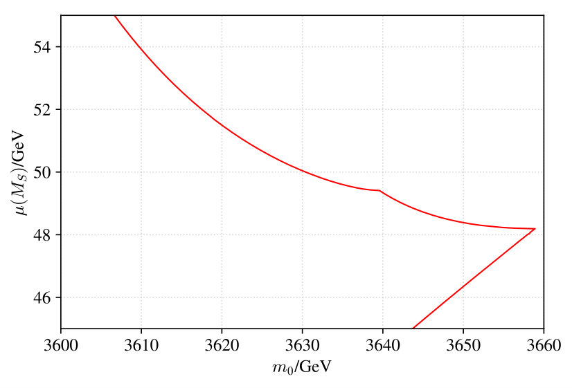 Figure 5
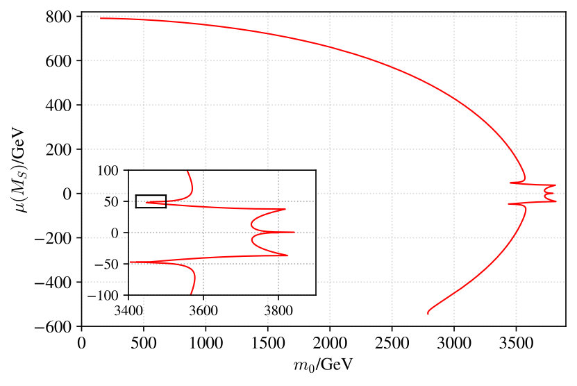 Figure 6
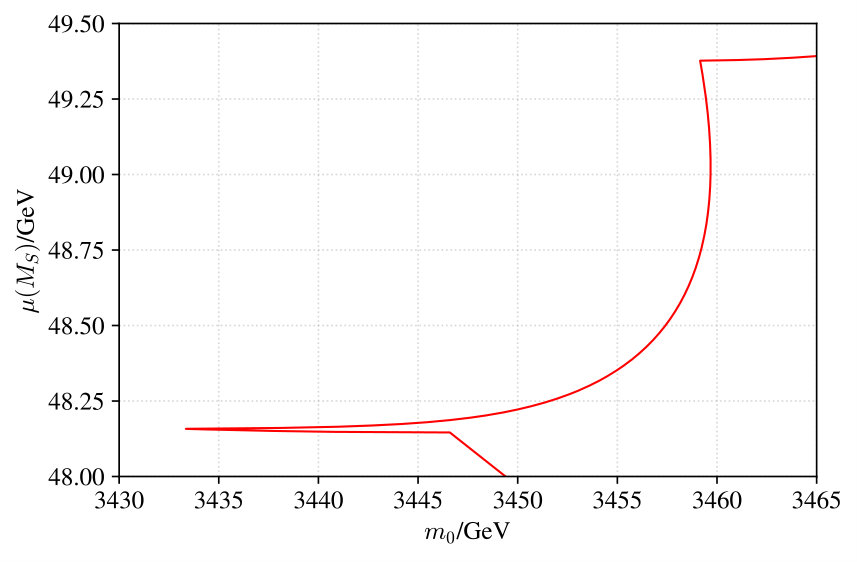 Figure 7
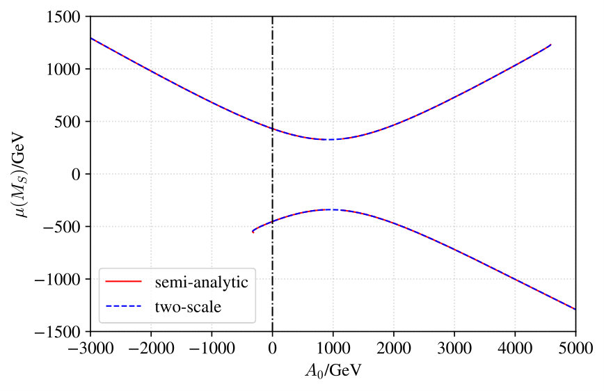 Figure 8
 Figure 9
 Figure 10
 Figure 11
 Figure 12
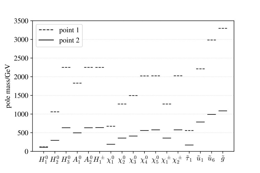 Figure 13
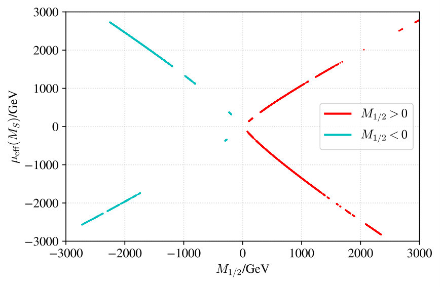 Figure 14
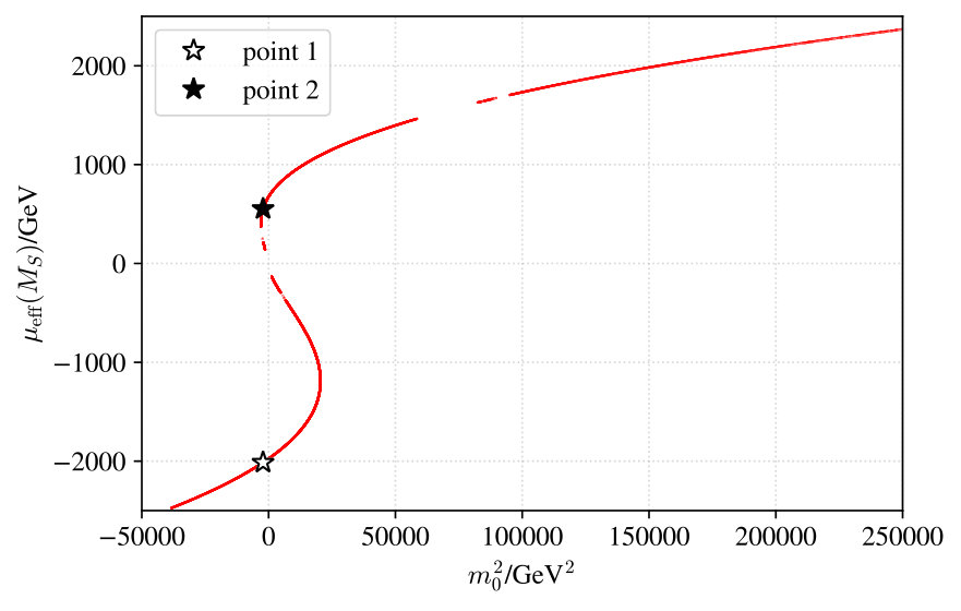 Figure 15
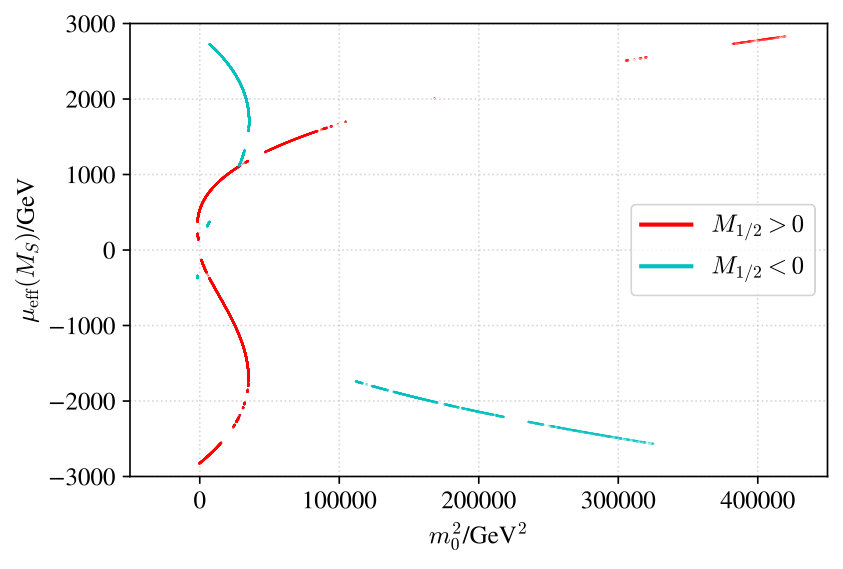 Figure 16
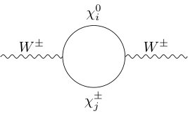 Figure 17
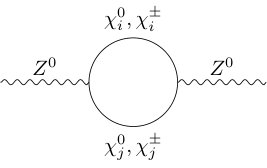 Figure 18
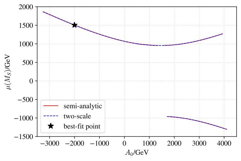 Figure 19
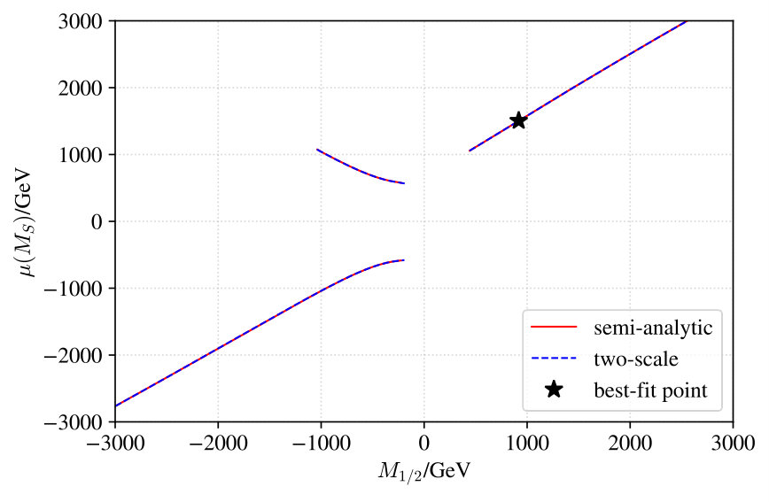 Figure 20
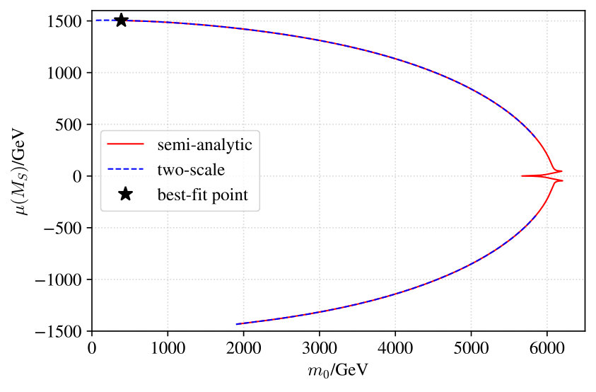 Figure 21
| solver | input | output |
|---|---|---|
| TSS | , , , | , |
| SAS1 | , , , | , |
| SAS2 | , , , | , |
| SAS3 | , , , | , |
| point 1 | point 2 | |
| /GeV | ||
| /GeV | ||
| /GeV | ||
| /GeV | ||
| /GeV | 673.3 | 189.7 |
| /GeV |
Peer Reviews
No public reviews on file for this paper yet. If you reviewed it on a platform where reviews are public (OpenReview, ICLR, NeurIPS, ICML), you can paste yours below so the community can read it here.
Videos
No videos yet. Explain this paper in a talk, walkthrough, or lecture? Add one.
∎
{textblock*}
10em(0.98) DESY 19-129
TTK–19–28
\thankstext
t1This research was supported by the German DFG Research Unit New Physics at the LHC (FOR 2239) and the German DFG Excellence Strategy Quantum Universe (EXC 2121). \thankstexte1e-mail: [email protected] \thankstexte2e-mail: [email protected]
11institutetext: Deutsches Elektronen-Synchrotron DESY, Notkestraße 85, 22607 Hamburg, Germany 22institutetext: Institute for Theoretical Particle Physics and Cosmology, RWTH Aachen University, 52074 Aachen, Germany
Investigating multiple solutions to boundary value problems in
constrained minimal and non-minimal SUSY models\thanksreft1
Daniel Meuser\thanksrefe1,addr1
Alexander Voigt\thanksrefe2,addr2
(Received: date / Accepted: date)
Abstract
We investigate the physical origins of multiple solutions to boundary value problems in the fully constrained MSSM and NMSSM. We derive mathematical criteria that formulate circumstances under which multiple solutions can appear. Finally, we study the validity of the exclusion of the CMSSM in the presence of multiple solutions.
Keywords:
MSSM NMSSM multiple solutions boundary value problem
††journal: Eur. Phys. J. C
1 Introduction
After the discovery of the Higgs boson with a mass of Aad:2012tfa ; Chatrchyan:2012xdj ; Aad:2015zhl and the non-discovery of supersymmetric (SUSY) particles at the LHC, it becomes clearer that pure weak-scale supersymmetry may not be realized in nature. Although the general Minimal Supersymmetric Standard Model (MSSM) may be difficult to fully exclude, the constrained MSSM (CMSSM), which is inspired by minimal supergravity, has been excluded at more than confidence level Bechtle:2015nua ; Athron:2017qdc . One reason for the exclusion is that in the CMSSM, by construction, all sfermion masses are of the same order. In this case, however, observables such as the Higgs boson mass, Dark Matter and the anomalous magnetic moment of the muon cannot be explained simultaneously by the MSSM, because requires multi-TeV stops, while the other observables prefer sub-TeV sleptons.
However, in Refs. Allanach:2013yua ; Allanach:2013cda ; Allanach:2014sea it was discovered that there may be multiple MSSM parameter sets which fulfill the same CMSSM boundary conditions. The mathematical reason for this phenomenon is that the CMSSM is formulated as a boundary value problem (BVP), where the running MSSM parameters are fixed by input values at different renormalization scales. The parameters at the different scales are connected via a set of differential equations, the so-called renormalization group equations (RGEs). Formally, such a BVP may have no, one, or multiple solutions for the MSSM parameters.
In order to make a statement about the validity of the CMSSM, all possible solutions to the BVP must be studied. However, the BVP solving algorithm used in the global fitting analyses of Refs. Bechtle:2015nua ; Athron:2017qdc can at most find one solution and may miss further ones. This raises the question whether the CMSSM is still excluded in the presence of multiple solutions of the BVP.
In the present paper we systematically study the physical origin of the multiple solutions in the CMSSM. In doing this, we go beyond the scope of Refs. Allanach:2013yua ; Allanach:2013cda and derive mathematical criteria that formulate circumstances under which multiple solutions can appear. In addition we study the influence of the chosen low-energy observables that fix the electroweak gauge couplings, which appear to play in important role for the occurrence and the number of multiple solutions. Next, we apply our newly gained insights to the results presented in Ref. Bechtle:2015nua and investigate the influence of multiple solutions on the global fit performed therein. Finally, we extend our analysis to the fully constrained Next-to-Minimal Supersymmetric Standard Model (CNMSSM) and demonstrate that multiple solutions can also occur in constrained non-minimal SUSY models.
2 Boundary value problems
2.1 CMSSM boundary conditions
The CMSSM is formulated as a BVP, where the parameters are fixed at three different scales, see Fig. 1. At the electroweak scale , the gauge and Yukawa couplings () and as well as the SM-like Higgs vacuum expectation value (VEV) are determined from known Standard Model observables and the ratio . At the gauge coupling unification scale (GUT scale) , defined by , the soft-breaking sfermion and Higgs mass parameters and (), the gaugino mass parameters as well as the trilinear couplings () are unified to
[TABLE]
At the SUSY scale , where denotes the -th stop mass, the parameters and are fixed by the two electroweak symmetry breaking (EWSB) equations. This leaves the following five free parameters of the CMSSM:
[TABLE]
2.2 CNMSSM boundary conditions
In the symmetric NMSSM the parameters and are absent and are replaced by the new parameters , , , , and Ellwanger:2009dp . In the following study we consider the fully constrained symmetric NMSSM (CNMSSM) Ellwanger:1993xa ; Ellwanger:1995ru ; Ellwanger:1996gw ; Djouadi:2008yj ; Djouadi:2008uj , where all soft-breaking parameters are unified at the GUT scale as in Eqs. (1) with the additional constraints
[TABLE]
see Fig. 2. This leaves seven free parameters , , , , , , and , of which three are fixed by the NMSSM EWSB equations. Since and are dimensionless parameters that enter all NMSSM functions at sufficiently high order, we take them as input at and fix the parameters , and by the three EWSB equations via the semi-analytic approach, see below. As a result, we are left with the following four free CNMSSM parameters:
[TABLE]
In the following we trade for .
2.3 Matching to low-energy observables
For the study of multiple solutions in the C(N)MSSM, the calculation of the electroweak gauge couplings and is of particular importance. In our analysis we use FlexibleSUSY 2.1.0 Athron:2014yba ; Athron:2017fvs , where the are determined from the electromagnetic fine-structure constant and the weak mixing angle as
[TABLE]
Since version 2.0.0, FlexibleSUSY offers the following two possibilities to calculate :
The pole mass and the Fermi constant can be chosen as input, in which case the weak mixing angle is calculated as
[TABLE]
where is a function of the one-loop and the self-energies Pierce:1996zz . 2. 2.
The pole mass and the pole mass can be chosen as input, in which case the weak mixing angle is calculated as
[TABLE]
In Eq. (7) and denote the and masses, respectively, calculated as
[TABLE]
with and being the corresponding one-loop vector boson self-energy.
Both Eqs. (6) and (7) are equivalent at the one-loop level, but differ at higher orders. The difference involves in particular products of the one-loop vector boson self-energies. This difference is of crucial importance for the existence of multiple solutions at small values of , as is shown in Sect. 3.1.
2.4 Boundary value problem solvers
The most common way to solve the CMSSM BVP is the “two-scale solver” (TSS), also known as “running and matching”. In this approach the spectrum generator numerically integrates the RGEs and imposes the boundary conditions at each scale in an iterative way. If the iteration converges, the algorithm has found one solution of the BVP. In the CMSSM one can use the TSS to choose , , , and as input and the parameters and become an output at the SUSY scale . As an illustration we show in Fig. 3 the relation between and for the parameter set Allanach:2013cda
[TABLE]
and for both signs of . The blue dashed line denotes all points where the TSS could find a solution. We see for instance that for the TSS could find a solution for , but not for . For the TSS finds one solution for each and for no solution is found.
The CNMSSM BVP, however, cannot be solved in this way with the TSS. There, if one chooses , , and as input at the GUT scale, the parameters , and would need to be fixed by the EWSB equations at the scale . Since and are dimensionless parameters which enter most NMSSM functions, the iteration between the scales becomes unstable and the TSS does not converge.
This downside of the TSS led to the development of the semi-analytic solver (SAS) Athron:2009ue ; Athron:2009bs ; Athron:2011wu ; Athron:2012sq ; Athron:2012pw ; Athron:2017fvs , which allows one to exchange the role of input and output parameters in constrained models. To achieve that, the SAS exploits the general structure of the RGEs to decompose the soft-breaking parameters in terms of GUT parameters and dimensionless coefficients Athron:2017fvs :
[TABLE]
The coefficients are scale dependent but independent of the (dimensionful) GUT parameters. They are determined numerically by solving the BVP for different values of , , , and with the TSS. Once the coefficients are known, Eqs. (10) can be solved for the soft-breaking parameters, which become an output of the algorithm.
The property of the SAS to exchange input and output parameters has several advantages over the TSS:
- •
If the relation between input and output parameters is not injective (which occurs in both the CMSSM and CNMSSM), scanning over one parameter while obtaining the other one as output, and vice versa, allows the search for multiple solutions of the BVP. This procedure is shown by the red solid line in Fig. 3, where is used as input and is output. One immediately sees that with the SAS one can find up to four solutions for around , which have not been found by the TSS. In Sect. 3 we use this procedure to study in depth the physical origin of the multiple solutions found in Refs. Allanach:2013yua ; Allanach:2013cda ; Allanach:2014sea .
- •
In models where the TSS would require dimensionless parameters to be output, as for example in the CNMSSM or CE6SSM Athron:2008np ; Athron:2009bs , the SAS enables one to take them as input, which yields a stable iteration between the high and low scales. In Sect. 4 we use this feature in the CNMSSM to take the parameters , , and as input and obtain , , and as output.
On the other hand, there are scenarios where it is advantageous to use the TSS:
- •
If the derivative approaches zero, as happens for example in Fig. 3 around , scanning over is no longer suitable. Invoking the TSS to vary instead and receiving as an output allows to study a region of parameter space which cannot be accessed via the SAS as easily.
- •
In cases where both solvers find the same unique solution it is a priori not clear whether the TSS or the SAS is the better choice. A combination of both allows a more complete study and a comparison validates the equivalence of the two solvers. In those cases, the TSS in general converges much faster than the SAS does.
In the following section we use the semi-analytic approach to systematically search for multiple solutions to the BVP of the CMSSM and study their origin in depth. For our analysis we use the SAS implemented in FlexibleSUSY 2.1.0. Athron:2014yba ; Athron:2017fvs .
3 Multiple solutions in the CMSSM
3.1 Effects from light SUSY particles
In this section we study the occurrence of multiple solutions in the CMSSM for small values of (see Fig. 3), which were first observed in Refs. Allanach:2013cda ; Allanach:2013yua . Without limitation of generality we restrict our analysis to positive values of by making use of the approximate mirror symmetry , which allows two values for for fixed as long as is not too large. As was shown in Refs. Allanach:2013cda ; Allanach:2013yua , even for fixed the function is not necessarily bijective: In the region the function has several turning points where the derivative exhibits singular behavior, see Figs. 4, for the input parameter choice . Interestingly, if is chosen as input, more solutions appear as shown in Figs. 5. In the following we analyze the origin of these singularities and derive a mathematical criterion that describes their positions and count.111The singularity at originates from a massless chargino entering the 1-loop threshold correction for . The region with is therefore strongly constrained by experimental data and is thus not discussed in the following.
First we consider the case where are chosen as input, see Figs. 4. In the enlarged subplot of Fig. 4 one finds one spike at . Zooming in further reveals one additional kink in Fig. 4 at . If are chosen as input (see Figs. 5), the shape of the curve is different: In the zoomed subplot in Fig. 5 one finds two spikes at and , respectively. Zooming in further reveals two additional kinks in Fig. 5 for and , respectively. In total one finds two kinks for positive for and four kinks for .
The origin of these kinks can be traced back to singular chargino and neutralino contributions to the one-loop vector boson self-energies and (see Fig. 6), which are used to calculate the electroweak gauge couplings at the scale , as described in Sect. 2.1. Since the gauge couplings contribute to every function of the MSSM, a singular point in translates into a singular point in . Note that the precise dependence of the on the depends on the chosen set of input parameters, or . This explains the different singularities between Figs. 4 and 5. In the following we describe the intricate dependence of and investigate the source of the singularities of .
The vector boson self-energies depend on via the chargino and neutralino masses, which enter the one-loop diagrams shown in Fig. 6. Expressed in terms the loop functions and Pierce:1996zz , each diagram gives a contribution
[TABLE]
to the self-energies. In Eq. (11) denotes the external momentum squared, are the running masses of the fermions in the loop, and and are vertex coefficients derived from the Lagrangian. All running quantities are evaluated at the renormalization scale . In total there are fourteen electroweakino diagrams contributing to and eight to . Of these, four () and two () contain only higgsino-like charginos and neutralinos, whose masses are approximately given by . Therefore, only those six diagrams are responsible for the kinks.
The singularities in now have the following deeper origin: In the renormalization scheme the finite part of the function appearing in Eq. (11) is given by
[TABLE]
where
[TABLE]
In Fig. 7 the real and imaginary part of are shown exemplary as a function of the mass for fixed . One finds that as soon as becomes small enough such that both particles in the loop go on-shell simultaneously, acquires an imaginary part and the derivatives of the real and the imaginary part are singular for this value of . This is due to the square root function in Eq. (13b) not being differentiable when its argument vanishes. The radicand, which is just the Källén function222 , has two roots
[TABLE]
of which the one with positive sign is located at and the one with negative sign is located at in Fig. 7. Both real and imaginary part are not differentiable at the zero , but they are at the other due to a cancellation between the -terms in Eq. (12). The appearance of an imaginary part is in accordance with the optical theorem from which we expect the self-energy to become complex when the particles in the loop are light enough to go on-shell simultaneously.
With this knowledge one would expect four higgsino-like (and thus -dependent) combinations (, , , ) to give rise to singularities in the self-energy, and two combinations () for the self-energy. Following, there should be four spikes for the input parameters and six for in total. However, there are only two and four spikes in , respectively. Evaluating Eq. (11) in the limit of a vanishing Källén function renders it in a form in which the disappearance of some singularities becomes manifest. To this end we use the identities
[TABLE]
where we have neglected constants as well as terms which are proportional to the one-point function Pierce:1996zz . Plugging Eqs. (15) in Eq. (11) and setting , we arrive at
[TABLE]
We plug the root Eq. (14) with positive sign into Eq. (16) to obtain
[TABLE]
Eq. (17) is the non-vanishing part of a self-energy graph in the limit where the Källén function is zero. From this we infer that whenever is zero in the limit , the corresponding diagram does not contribute a singularity to .
Since the entries of the chargino mixing matrices and are independent, there is no relation which would guarantee the cancellation , as long as at least one chargino appears in the loop. Hence, the diagrams with , , and in the loop contribute non-vanishing singularities to .
The other three relevant diagrams are pure contributions to the self-energy. For a vertex the relation holds Pierce:1996zz . Since the are in general complex quantities, this property is not sufficient for to vanish. If the neutralinos are identical, however, and become real and cancel when added.
We conclude that the self-energy diagrams with identical neutralinos in the loop do never give a spike, since the singular terms in have a vanishing coefficient in the limit . The singularities (kinks or spikes) originate only from diagrams with light , , , or in the loop.
Note, that at the singular points spikes or kinks can appear in the overall vector boson self-energies. However, only spikes lead to multiple solutions, because there the sign of the derivative around the singular point changes, which results in a turning point. Whether a singularity causes a spike or a kink depends on the relative sign between the function which causes the singularity and other loop corrections to the self-energy. The relative signs generally depend on the regarded model as well as on the input parameters.
3.2 Effects from non-linear parameter inter-dependencies
In Refs. Allanach:2013cda ; Allanach:2013yua another CMSSM parameter region with multiple solutions was found around , see Fig. 8. In this section we investigate this parameter region with multiple solutions, which we find are not caused by light particles in vector boson self-energies, but by intricate nonlinear parameter inter-dependencies.
The non-monotonic behavior of in the region is depicted in Fig. 8. Multiple solutions appear in this region, because the function changes its sign such that has a minimum at . For too small values of there is no physical solution because the running masses of the neutral Higgs bosons become tachyonic in this region of parameter space. In the following we study the parameter interplay which is responsible for the existence of the minimum.
To this end, we derive an approximate relation between and . Our starting point is the tree-level EWSB equation
[TABLE]
which is imposed at the SUSY scale . Hence, all renormalization scale dependent quantities are evaluated at . For our set of input parameters, holds and we can also neglect the -term, which implies
[TABLE]
To relate those parameters to , we make use of the RGEs
[TABLE]
At leading order the functions are independent of and fulfill the hierarchy . This hierarchy arises because the up-type function is proportional to the squared top-Yukawa coupling whereas the down-type one contains only down-type fermion contributions. It causes to be close to and at the same time allows to become negative—which is usually necessary for EWSB to occur. We will therefore only replace in Eq. (19) by Eq. (20) and arrive at
[TABLE]
This, to leading order, implies that a minimum of appears when
[TABLE]
For our choice of parameters, a numerical analysis leads to
[TABLE]
so Eq. (22) is fulfilled for . A comparison with Fig. 8 validates that this indeed is the position of the minimum around which multiple solutions occur. For differently chosen input parameters the existence of a point where the derivative of is of the appropriate size to create a minimum is not ensured. An example for this is given in Sect. 3.4.
3.3 Multiple solutions for and
The SAS allows one to exchange input and output parameters of constrained (SUSY) models. This property was used in the previous sections to exchange the role of and in the CMSSM to examine the function for (non-)injectivity. However, the SAS is not restricted to the exchange (SAS1) and further choices are possible, see Table 1. In the following we apply the SAS to study the relations (SAS2) and (SAS3) to investigate the implications of their non-bijectivity.
The semi-analytic solver can treat the GUT parameter as output and as input (SAS2) by solving the EWSB equations for . To do so, one makes use of the semi-analytic ansatz Eqs. (10) again. The equation involving the is quadratic in , in contrast to being linear in , which allows for up to two distinct solutions for fixed . In Figs. 9(a) and 9(b) we scan over (SAS2) and (TSS) for , and two different values . As expected, the semi-analytic solver finds two branches, one for each solution of the quadratic equation. The TSS only finds solutions which are obtained from SAS2 as well. The solutions at (vertical black lines) are the same as found in Sect. 3.1 using SAS1. Thus, scanning over while using as an output parameter does not give new solutions compared to the case where is output.
Similarly to SAS2, can be treated as output parameter by solving the EWSB equations for (SAS3) instead. Also in this case the ansatz is quadratic in , so up to two distinct solutions are possible. In Figs. 10(a) and 10(b) we show and for , , and . We find that for (Fig. 10(b)) the SAS can scan over both solution branches, while for (Fig. 10(a)) the two branches have merged. The multiple solutions around have vanished and a region without solutions () has emerged. The curve becomes flat around and SAS3 is not suitable to find solutions in the region where the two solution branches merge; the two-scale solver, however, is able to find more solutions in this case. Besides this, the multiple solutions that we obtain for SAS3 are again the same as found for SAS1 in Sect. 3.1.
In conclusion, scanning over while receiving either or as output does not give us any new solutions compared to the output search strategy. We nevertheless have been able to reproduce the previous results in a consistent manner and also our expectation of finding two branches of solutions for parameters of mass dimension one has been fulfilled. Furthermore, the same singular structures for small values of have appeared for SAS2 and SAS3. Note also, that both the two-scale and the semi-analytic solver had to be used to find all solutions in the considered parameter regions.
3.4 Is the CMSSM still excluded?
In this section we investigate the relevance of multiple solutions for globally fitting the CMSSM to experimental and observational data. As a reference point we use Ref. Bechtle:2015nua (“Killing the CMSSM softly”), in which the program Fittino was used. The idea was to scan over a reasonable region of the CMSSM input parameter space and to determine the fit point which is the most compatible with the considered observables. Furthermore, this paper was the first to derive a consistent -value for the CMSSM from toy experiment.
3.4.1 The Results of “Killing the CMSSM Softly”
We briefly list the observables which have been used in the analysis of Ref. Bechtle:2015nua . As for the precision observables there are the anomalous magnetic moment of the muon , the effective weak mixing-angle , the top quark and boson masses as well as the b quark/B meson branching ratios. Additionally, different combinations of Higgs observables, like e.g. the SM Higgs boson mass and its decay channels, as observed by the ATLAS/CMS experiments at the LHC, and the dark matter relic density , as measured by the Planck collaboration, are incorporated.
The following parameter values were found to give the best accordance between measured and predicted observables and are hereinafter referred to as “best-fit point” parameters:
[TABLE]
It should be noted that these values were determined with the spectrum generators SPheno 3.2.4 Porod:2003um ; Porod:2011nf and FeynHiggs 2.10.1 Heinemeyer:1998yj ; Heinemeyer:1998np ; Degrassi:2002fi ; Frank:2006yh ; Hahn:2013ria ; Bahl:2016brp ; Bahl:2017aev ; Borowka:2014wla ; Heinemeyer:2007aq ; Hollik:2014bua ; Hollik:2015ema , whereas the following analysis is based on the predictions of FlexibleSUSY 2.1.0.
For these input parameters and 333The solution with negative is located in an unphysical region where the -odd Higgs boson becomes tachyonic. FlexibleSUSY finds
[TABLE]
The chargino masses are determined by and . The lightest chargino is thus able to escape the LEP bound Tanabashi:2018oca . The lightest supersymmetric particle (LSP) is the lightest neutralino with mass and provides a dark matter candidate. At the best-fit point the predicted dark matter relic density is in agreement with the experimental observations.
The Standard Model prediction for the anomalous magnetic moment of the muon deviates from the observed value at a level. To account for this, a successful SUSY model is expected to give an additional contribution to of the order Davier:2010nc . The best-fit point predicts a correction , which is far too small.
Ref. Bechtle:2015nua concludes by giving the following -value for the CMSSM:
[TABLE]
When performing a global fit of a model to known observables, all possible mathematical solutions to the formulated boundary value problem need to be taken into account. The TSS of SPheno, however, which was used in Ref. Bechtle:2015nua , does not necessarily find all solutions. For this reason we study in the following section whether further solutions to the CMSSM BVP can be found around the best-fit point with the semi-analytic approach.
3.4.2 Multiple Solutions around the Best-Fit Point
In this section we perform an analysis similar to the one of Sect. 3.3 for the best-fit point (cf. Eq. (24)). All except one of the free CMSSM GUT input parameters are set to their best-fit values and the remaining parameter is varied subsequently with the TSS of FlexibleSUSY. To find possible multiple solutions we repeat the same procedure but scan over by means of the semi-analytic solvers SAS1–SAS3. The results are shown in Figs. 11.
As for Fig. 11 we recognize the same overall relation between and as in Fig. 3 and the multiple solutions around appear as well. At the lower end of the curve, the multiple solutions due to non-linear parameter inter-dependencies are non-existent. There, for instance,
[TABLE]
and so Eq. (22) is not fulfilled.
In Figs. 11 and 11 the semi-analytic solver does not find any additional solutions compared to the two-scale solver. In the case of Fig. 11 the curve becomes too flat around to allow an efficient scan over with the SAS3. For some values of the scan parameters, for instance the region where in Fig. 11, we do not find a physical solution due to either tachyonic down-type sleptons, up-type squarks, or Higgs bosons.
Concluding, we find that the best-fit point is far off from the regions in which multiple solutions can occur. One reason is that around the best-fit point all SUSY particles are heavy enough to escape the experimental constraints, while our previous analysis has shown that additional solutions tend to occur in regions of parameter space where at least some superpartners become light.
4 Multiple solutions in the CNMSSM
In this section we study the occurrence of multiple solutions for a given set of parameters , , in the CNMSSM. Exchanging with allows us to search for multiple solutions in a similar fashion as we did for the CMSSM. It has to be noted, however, that we now also take the GUT parameters and to be output of our algorithm and not input as we did in the CMSSM.
4.1 Study of multiple solutions with the semi-analytic approach
As described in Sect. 2.2, the CNMSSM is formulated as a BVP with the universal GUT parameters , , . In order to study multiple solutions in the CNMSSM, we make use of the semi-analytic equations, which allows us to take the SUSY scale parameters , , as input. Specifying the dimensionless quantities and yields a good stability of the underlying solving algorithm. can now be used as a scan parameter as was done for the CMSSM. As a result, we formulate the CNMSSM BVP in terms of the input parameters
[TABLE]
and obtain , , as output.
In Figs. 12 we show a scan over for fixed values of , , and . The output parameters , , are shown on the abscissae. The curves are discontinuous due to the existence of two distinct solutions branches, which differ from each other in their sign of . In order to distinguish the branches, solutions with are marked as red and cyan dots, respectively. If we were able to pre-select one of the branches, a scan should yield a continuous relation between the output parameters and .
In contrast to the CMSSM, where we found multiple solutions, now we do not find any physical solutions in the parameter region at all. The reason for this is that, in our scenario, as tends to 0, the dimensionful output parameters become small and tachyons appear in the particle spectrum, i.e. the solutions of the BVP have to be discarded. Furthermore we find a highly non-linear dependence of on for each , see Fig. 12, which results in up to three solutions around . This non-linear dependence can be understood as follows: When determining the three GUT parameters from the three EWSB equations of the CNMSSM, the strongest restriction to the value of comes from the equation Ellwanger:2009dp
[TABLE]
For small and , the parameters and are approximately constant between the GUT and the EW scale Djouadi:2008uj , i.e. and . To obtain while keeping small, we have to allow for and can approximate
[TABLE]
From Fig. 12 we can also see with some positive function , which depends only weakly on , and so
[TABLE]
for . The term with positive sign is only approximately quadratic in and takes the shape of a slightly tilted parabola. It is the sum of both terms which causes the function to behave in the observed non-monotonic way.
The relation between and is nearly linear, as one would expect for two parameters of mass dimension one. The two branches with different are related to one another by an approximate central symmetry, see Fig. 12. The reason for the resulting discontinuous cross-like shape is that, as explained above, for a given value of the semi-analytic solver usually can find a solution for one value of , but not simultaneously for the opposite one. A similar behavior can be found for in Fig. 12, where the semi-analytic solver can find one solution for fixed at most. Here, however, the sign of is fully determined by the sign of and the output parameter differs only slightly between the two solution branches.
4.2 Mass spectra for two different solutions of a single
CNMSSM parameter point
In order to see the importance of multiple solutions in the CNMSSM, we compare the mass spectra of two different solutions for the parameter point
[TABLE]
The two solutions share the same , but have different , and , see Table 2 and Figs. 13.
As a result, the points have different pole mass spectra as shown Fig. 13. By comparing the predicted Higgs boson pole masses with the experimentally measured value of , point 2 can be excluded, while point 1 may still be taken into consideration. However, none of the points can correctly predict the observed Dark Matter relic density because the lightest stau is the lightest supersymmetric particle (LSP). This is in agreement with the analysis of Ref. Djouadi:2008uj , finding that the condition must be fulfilled in order for a CNMSSM parameter point to produce the observed dark matter relic density.
In any case, our analysis shows that the different solutions can have a significantly different phenomenology and the SAS is a useful tool to find and study multiple solutions in this model. However, since and are output parameters in our SAS formulation of the CNMSSM BVP, viability conditions such as the ones given in Ref. Djouadi:2008uj cannot be enforced from the start and have to be tested on the output parameters.
5 Conclusions
In Refs. Allanach:2013yua ; Allanach:2013cda ; Allanach:2014sea the appearance of multiple solutions to the BVP of the CMSSM has been discovered and studied. In the present paper we have investigated the deeper origin of these multiple solutions. The study was made possible by the semi-analytic BVP solver implemented in FlexibleSUSY, which allows to exchange input and output parameters to search for turning points of inverse functions of the BVP and thus allows the systematic search for multiple solutions. We could trace their appearance back to two phenomena:
- •
Light neutralinos and charginos can lead to singular points in the one-loop and self-energies, which translate to singular points in the function . At these points the derivative of can change its sign, which leads to multiple branches in the inverse functions . The position of the singular points is given by the light neutralino/chargino masses. The number of singular points depends on their couplings to the and bosons and on the formulation used to determine the weak mixing angle from physical observables.
- •
A non-linear inter-dependence between the parameters and can lead to a minimum of the function , resulting in the appearance of multiple branches in the inverse function around that minimum.
Furthermore we have answered the question whether the CMSSM is still excluded in the presence of potential multiple solutions. We find that around the CMSSM best-fit point the solution to the BVP is unique and thus the -value for the CMSSM remains at 4.9%.
Finally we have investigated the appearance of multiple solutions in the CNMSSM. We find that:
- •
Multiple solutions around tend to not occur, because in the limit also and other supersymmetry-breaking parameters vanish or become of the order of the electroweak scale, which leads to light or tachyonic scalar particles, i.e. unphysical solutions of the BVP.
- •
For small up to three solutions for can occur due to a non-linear inter-dependence between these two parameters, imposed by the EWSB equations and the functions. The different solutions may have significantly different physical spectra because of different values for , and .
Concluding, we would like to emphasize that in order to investigate the validity of a constrained SUSY model all possible solutions to the BVP must be studied. In combination with the conventional “running and matching” procedure (TSS), the semi-analytic approach (SAS) is a useful tool to search for additional solutions.
Acknowledgements.
We kindly thank Ben Allanach, Peter Athron, Dylan Harries and Werner Porod for helpful discussions.
The reference list from the paper itself. Each links out to its DOI / PubMed record.
- 1(1) G. Aad, et al., Phys. Lett. B 716 , 1 (2012). DOI 10.1016/j.physletb.2012.08.020
- 2(2) S. Chatrchyan, et al., Phys. Lett. B 716 , 30 (2012). DOI 10.1016/j.physletb.2012.08.021
- 3(3) G. Aad, et al., Phys. Rev. Lett. 114 , 191803 (2015). DOI 10.1103/Phys Rev Lett.114.191803
- 4(4) P. Bechtle, et al., Eur. Phys. J. C 76 (2), 96 (2016). DOI 10.1140/epjc/s 10052-015-3864-0
- 5(5) P. Athron, et al., Eur. Phys. J. C 77 (12), 824 (2017). DOI 10.1140/epjc/s 10052-017-5167-0
- 6(6) B.C. Allanach, D.P. George, B. Nachman, JHEP 02 , 031 (2014). DOI 10.1007/JHEP 02(2014)031
- 7(7) B.C. Allanach, D.P. George, B. Gripaios, JHEP 07 , 098 (2013). DOI 10.1007/JHEP 07(2013)098
- 8(8) B.C. Allanach, Phil. Trans. Roy. Soc. Lond. A 373 (2032), 0035 (2014). DOI 10.1098/rsta.2014.0035