Dynamically generated inflationary two-field potential via non-Riemannian volume forms
David Benisty, Eduardo I. Guendelman, Emil Nissimov, Svetlana Pacheva

TL;DR
This paper presents a modified gravity model with a non-Riemannian volume form that naturally generates a two-field inflationary potential, leading to slow-roll inflation consistent with observations and a stable dark energy minimum.
Contribution
It introduces a novel two-scalar-field potential derived from non-Riemannian volume forms, unifying inflation and dark energy within a single framework.
Findings
The model produces a large flat inflationary region with slow-roll behavior.
Numerical results for spectral index and tensor-to-scalar ratio match observational data.
The potential has a stable minimum corresponding to dark energy.
Abstract
We consider a simple model of modified gravity interacting with a single scalar field with weakly coupled exponential potential within the framework of non-Riemannian spacetime volume-form formalism. The specific form of the action is fixed by the requirement of invariance under global Weyl-scale symmetry. Upon passing to the physical Einstein frame we show how the non-Riemannian volume elements create a second canonical scalar field and dynamically generate a non-trivial two-scalar-field potential with two remarkable features: (i) it possesses a large flat region for large describing a slow-roll inflation; (ii) it has a stable low-lying minimum w.r.t. representing the dark energy density in the "late universe". We study the corresponding two-field slow-roll inflation and show that the pertinent slow-roll inflationary curve…
Click any figure to enlarge with its caption.
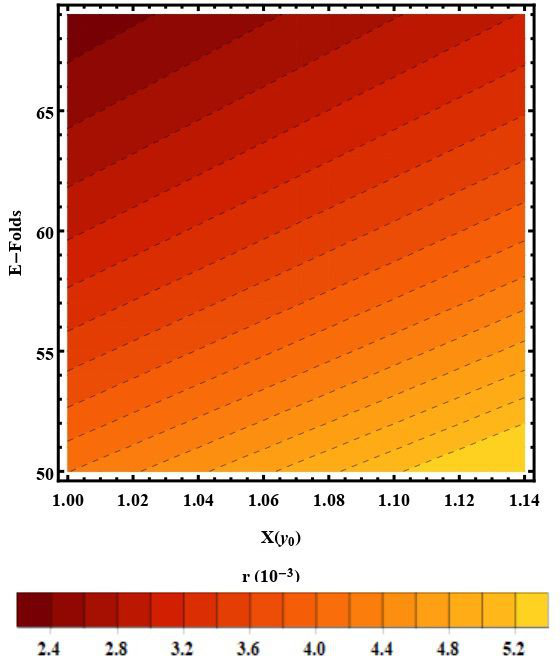 Figure 1
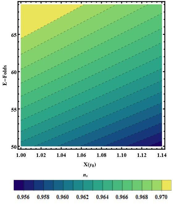 Figure 2
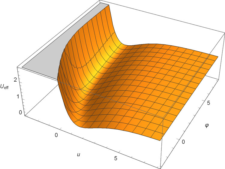 Figure 3
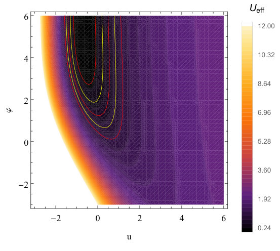 Figure 4
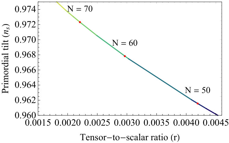 Figure 5
Peer Reviews
No public reviews on file for this paper yet. If you reviewed it on a platform where reviews are public (OpenReview, ICLR, NeurIPS, ICML), you can paste yours below so the community can read it here.
Videos
No videos yet. Explain this paper in a talk, walkthrough, or lecture? Add one.
Dynamically generated inflationary two-field potential via non-Riemannian volume forms
D. Benisty, E. I. Guendelman E. Nissimov and S. Pacheva
Physics Department, Ben-Gurion University of the Negev, Beer-Sheva 84105, Israel
*Frankfurt Institute for Advanced Studies (FIAS), Ruth-Moufang-Strasse 1, 60438 Frankfurt am Main, Germany
Bahamas Advanced Study Institute and Conferences, 4A Ocean Heights, Hill View Circle, Stella Maris, Long Island, The Bahamas*
Institute for Nuclear Research and Nuclear Energy, Bulgarian Academy of Sciences, Sofia, Bulgaria
We consider a simple model of modified gravity interacting with a single scalar field with weakly coupled exponential potential within the framework of non-Riemannian spacetime volume-form formalism. The specific form of the action is fixed by the requirement of invariance under global Weyl-scale symmetry. Upon passing to the physical Einstein frame we show how the non-Riemannian volume elements create a second canonical scalar field and dynamically generate a non-trivial two-scalar-field potential with two remarkable features: (i) it possesses a large flat region for large describing a slow-roll inflation; (ii) it has a stable low-lying minimum w.r.t. representing the dark energy density in the “late universe”. We study the corresponding two-field slow-roll inflation and show that the pertinent slow-roll inflationary curve in the two-field space has a very small curvature, i.e., changes very little during the inflationary evolution of on the flat region of . Explicit expressions are found for the slow-roll parameters which differ from those in the single-field inflationary counterpart. Numerical solutions for the scalar spectral index and the tensor-to-scalar ratio are derived agreeing with the observational data.
Contents
- 1 Introduction
- 2 Modified Gravity-Matter Model with Non-Riemannian Volume Elements
- 3 Applications to Cosmology
- 4 Conclusions
- 5 Acknowledgments
1 Introduction
Developments in cosmology have been inspired by the idea of inflation [1]-[5] which provides an attractive solution to the the horizon and the flatness problems. It provides in addition a framework for sensible calculations of primordial density perturbations [6]-[7] which becomes more and more interesting due to new data from the Cosmic Microwave Background. Dynamically generated models of inflation from modified/extended gravity such as the Starobinsky model [2] (see also the reviews [8, 9]) still remain viable and produce some of the best fits to existing observational data compared to other inflationary models [10].
Another efficient way to produce consistent inflationary models dynamically from modified/extended gravitational theories is based on employing alternative non-Riemannian spacetime volume-forms, i.e., metric-independent generally covariant volume elements, in the coresponding Lagrangian actions instead of the canonical Riemannian volume element given by the square-root of the determinant of the Riemannian metric (for recent applications of this idea, see [11, 12]). The method of metric-independent volume elements was originally proposed in [13]-[17]) with a subsequent concise geometric formulation in [18, 19].
The non-Riemannian volume element formalism was used as a basis for constructing (i) a series of extended gravity-matter models describing unified dark energy and dark matter scenario [20, 21]; (ii) quintessential cosmological models with gravity-assisted and inflaton-assisted dynamical suppression (in the “early” universe) or dynaamical generation (in the post-inflationary universe) of electroweak spontaneous symmetry breaking and charge confinement [22, 23, 24]; (iii) a novel mechanism for the supersymmetric Brout-Englert-Higgs effect in supergravity [18].
Let us briefly recall the essence of the non-Riemannian volume-form (volume element) formalism. In integrals over differentiable manifolds (not necessarily Riemannian one, so no metric is needed) volume-forms are given by nonsingular maximal rank differential forms :
[TABLE]
(our conventions for the alternating symbols and are: and ). The volume element transforms as scalar density under general coordinate reparametrizations.
In Riemannian -dimensional spacetime manifolds a standard generally-covariant volume-form is defined through the “D-bein” (frame-bundle) canonical one-forms ():
[TABLE]
To construct modified gravitational theories as alternatives to ordinary standard theories in Einstein’s general relativity, instead of we can employ one or more alternative non-Riemannian volume element(s) as in (1.1) given by non-singular exact -forms where:
[TABLE]
Thus, a non-Riemannian volume element is defined in terms of the (scalar density of the) dual field-strength of an auxiliary rank tensor gauge field .
2 Modified Gravity-Matter Model with Non-Riemannian Volume Elements
Let us consider the following specific modified model of gravity coupled to a real scalar field , constructed within the non-Riemannian spacetime volume-form formalism and involving several non-Riemannian volume elements, with an action (for simplicity we are using units with the Newton constant ):
[TABLE]
Here the following notations are used:
- •
is the scalar curvature of the Riemannian spacetime metric ; ;
- •
We employ three metric-independent volume-elements built in terms of auxiliary rank 3 antisymmetric tensor gauge fields:
[TABLE]
- •
The matter Lagrangian of a single scalar is given in two pieces:
[TABLE]
where and are dimensionful (positive) coupling parameters; will be considered small parameter.
- •
is dimensionfull parameter to be identified as energy density scale of the inflationary universe’ epoch.
The specific form of the action (2.4) is dictated by the requirement about global Weyl-scale invariance111Scale invariance played an important role since the original papers on the non-canonical volume-form formalism [15]. Also let us note that spontaneously broken dilatation symmetry models constructed along these lines are free of the Fifth Force Problem [17]. under:
[TABLE]
The modified gravitational theories of the type (2.4), when formulated within the first-order (Palatini) formalism, possess the following characteristic feature. The auxiliary rank 3 tensor gauge fields defining all non-Riemannian volume-elements (2.5) are almost pure-gauge degrees of freedom, i.e. they do not introduce any additional propagating gravitational degrees of freedom when passing to the physical Einstein frame except for few discrete degrees of freedom with conserved canonical momenta appearing as arbitrary integration constants. This has been explicitly shown within the canonical Hamiltonian treatment (see Appendices A in Refs.[19, 22]).
Unlike Palatini formalism, when we treat (2.4) in the second order (metric) formalism, while passing to the physical Einstein frame via conformal transformation:
[TABLE]
the first non-Riemannian volume element in (2.4) is not any more (almost) “pure gauge”, but creates a new dynamical canonical scalar field via . In Ref.[12] we have shown how, starting from a purely gravitational model within the non-Riemannian volume element formalism without any coupling to matter fields (i.e., starting with an action (2.4) where identically), the passage to the physical Einstein frame produces a non-trivial inflationary potential for the dynamically created scalar field . Here below, this idea is extended to produce dynamically a non-trivial two-field inflationary potential starting from the single-scalar-field action (2.4).
The equations of motion upon variation of (2.4) w.r.t. the auxiliary tensor gauge fields yield, respectively, the following solutions:
[TABLE]
Let us note that Eqs.(2.10) are (non-dynamical) constraints, whereas Eq.(2.9) is a dynamical relation – it contains second-order time derivatives inside .
In (2.9)-(2.10) and are (dimensionful and dimensionless, respectively) free integration constants. The appearance of indicate spontaneous breaking of global Weyl symmetry (2.7).
Accordingly, the equations of motion w.r.t. taking into account Eqs.(2.10) read:
[TABLE]
with as in (2.8).
We now transform Eqs.(2.11) via the conformal transformation (2.8) and show that the transformed equations acquire the standard form of Einstein equations w.r.t. the new “Einstein-frame” metric . To this end we will use the known formulas for the conformal transformations of and for some arbitrary scalar field, in particular (see e.g. Ref.[25]; bars indicate magnitudes in the -frame):
[TABLE]
and
[TABLE]
Indeed, using (2.12)-(2.13) and taking into account all relations (2.9) and (2.10), then Eqs.(2.11) are rewritten in the standard Einstein’s form of w.r.t. the “Einstein-frame” metric :
[TABLE]
where we have redefined:
[TABLE]
in order to obtain a canonically normalized kinetic term for the scalar field , and where:
[TABLE]
The corresponding Einstein-frame action reads:
[TABLE]
Let us note that we could obtain the Einstein-frame action (2.17) directly from the initial action (2.4) in the non-Riemannian volume-form formalism upon performing there the conformal transformation from to (2.8). To this end one has to use the known formula for the conformal transformation (2.8) of the scalar curvature (e.g., Ref.[25]):
[TABLE]
and then repeat the same steps as in Ref.[11], where such a procedure has been applied to a simplified version of the original action (2.4).
Let us particularly stress that the Einsten-frame action (2.17) contains a dynamically created canonical scalar field entering a non-trivial effective two-field scalar potential (2.16) – both are dynamically produced by the initial non-Riemannian volume elements in (2.4) due to the appearance of the free integration constants in their respective equations of motion (2.9)-(2.10).
The form of is graphically depicted on Fig.1 .
3 Applications to Cosmology
From cosmological point of view the dynamically generated two-field scalar potential (2.16) possesses the following relevant features:
- •
For large positive , , i.e., almost flat region regardless of .
- •
has a stable minimum at certain finite values .
Indeed, calculating the extremal point(s):
[TABLE]
we find for the matrix of second derivatives of at the extremal point :
[TABLE]
which is manifestly positive definite (both the diagonal elements as well as its determinant \frac{\alpha^{2}}{3}\bigl{(}f_{1}^{2}/\chi_{2}f_{2}\bigr{)}\,\bigl{(}M_{1}^{2}/\chi_{2}M_{2}\bigr{)} are all positive).
The flat region of for large positive corresponds to “early” universe’ slow-roll inflationary evolution with energy scale . On the other hand, the region around the stable minimum at (3.19) corresponds to “late” universe’ evolution where the minimum value of the potential:
[TABLE]
is the dark energy density value [29, 30, 31]. Thus, to conform to the observational data and we can choose for instance::
[TABLE]
where is the electroweak scale and is the Planck mass.
Let us now consider reduction of the Einstein-frame action (2.17) to the Friedmann-Lemaitre-Robertson-Walker (FLRW) setting with metric , and with , .
On the flat region of for large positive (henceforth we will use the notation for simplicity) the slow-roll dynamics:
[TABLE]
where denotes the Hubble parameter , defines an inflationary trajectory in the two-field space which can be described as a curve satisfying:
[TABLE]
Assuming small, Eq.(3.26) can be solved as:
[TABLE]
where:
[TABLE]
with and being an integration constant. Comparing (3.27) with the explicit expression (3.28) requires for consistency in the inflationary region (flat region for large positive ) that the integration constant must also be large positive.
We notice that (2.16) and (3.24), (3.25) all depend on only through \bigl{(}x\equiv e^{-u/\sqrt{3}},y\equiv e^{-\alpha\varphi}\bigr{)}, therefore it will be convenient to consider them as functions of :
[TABLE]
(here ). Accordingly, the inflationary curve will be represented as a curve in space satisfying the counterpart of Eq.(3.26):
[TABLE]
and the solution of Eq.(3.30) is obtained as power series w.r.t. a very small parameter :
[TABLE]
Henceforth we will keep as zero-order term in the -expansion of (3.31).
Following the geometric description of two-field inflationary trajectories in Ref.[26], Eqs.(3.30)-(3.32) mean that the present inflationary curve has a very small curvature:
[TABLE]
(i.e., very small turn rate) because of the small coupling parameter , and thus is close to an inflation along the -field direction.
Taking into account (3.27)-(3.28) (or their counterparts (3.31)-(3.32)) and (recall \bigl{(}x\equiv e^{-u/\sqrt{3}},\,y\equiv e^{-\alpha\varphi}\bigr{)}):
[TABLE]
the standard slow-roll parameters:
[TABLE]
can be written as functions of upto terms of order :
[TABLE]
where we used the short-hand notations:
[TABLE]
The end of the inflation occurs for or when in (3.36) becomes (discarding terms of order ):
[TABLE]
with as in (3.37) for .
Using relation (3.21) for and ignoring the very small value of , becomes:
[TABLE]
where the upper limit in the last inequality is implied by the reality of (3.38). Let us particularly note, that the expression and inequality (3.39) explicitly exhibits the difference between the present two-field inflation (even when discarding the -corrections) and its single field -inflation counterpart, where (upon ignoring ), cf. Ref.[12].
For the number of e-folds using we have
[TABLE]
which can be represented as:
[TABLE]
where and correspond to start and end of inflation.
Using the -expansion for (3.31) we obtain from (3.41), using again relation (3.21) for (and discarding the very small ) as well as the short-hand notation for (3.39):
[TABLE]
where and with as in (3.37) and given by Eq.(3.38).
Through the expressions for the slow-roll parameters (3.36) and the number of e-folds (3.42) one can calculate the values of the scalar spectral index and the tensor-to-scalar ratio, respectively, as functions of the number of e-folds [27, 28]:
[TABLE]
Unlike the case of single-field -inflation [12], now the results will parametrically depend on the value of through . Fig.2 contains contour plots for the predicted values of the and for different -foldings, with different allowed values of . All of the observables fit within the PLANCK data with the constraints [10]:
[TABLE]
however in future the observables are going to be more constrained. The future Euclid and SPHEREx missions or the BICEP3 experiment are expected to provide experimental evidence to test those predictions.
4 Conclusions
In the present paper we propose a simple model of modified gravity interacting with a single scalar field weakly coupled via exponential potential. The construction is based on the formalism of non-Riemannian spacetime volume-elements. In addition, the structure of the initial action is specified by the requirement of invariance under global Weyl-scale symmetry. Since we are employing the second order (metric) formalism for the gravity part of the action, the transition from the original frame with the non-Riemannian volume elements to the physical Einstein frame creates dynamically a second canonical scalar field accompanied by the emergence of several free integration constants. All this leads to the dynamical generation of a non-trivial two-scalar-field potential . We show that the dynamically created field serves as an inflaton field in the region of slow-roll inflation which is a flat region of the potential for large . Furthermore, we explicitly show that possesses a stable very low lying minimum as function of appropriate to describe the dark energy dominated “late” universe with a very small dark energy density.
We show that the pertinent slow-roll inflationary curve in -space has very small curvature in a sense that changes very little during the inflationary evolution of . We find an analytic solutions to the observables – scalar to tensor ratio and the scalar spectral index , which fit the known observational data. Beyond this prediction, the interaction between the two scalarfields leads to different values of the observables, which in future experiments will be constrained more efficiently. In what follows we intend to study the two-field inflationary evolution curve relaxing the assumption of weakly coupled , especially in the context of the non-Gaussianity feature in CMB (for recent review, see [32] and references therein) , which might provide more justification for the viability of the present model.
5 Acknowledgments
We gratefully acknowledge support of our collaboration through the Exchange Agreement between Ben-Gurion University, Beer-Sheva, Israel and Bulgarian Academy of Sciences, Sofia, Bulgaria. E.N. and S.P. are thankful for support by Contract DN 18/1 from Bulgarian National Science Fund. D.B., E.G. and E.N. are also partially supported by COST Actions CA15117, CA16104 and CA18108. D.B., E.N. and S.P. acknowledge illuminating discussions with Lilia Anguelova. Finally, we thank the referee for constructive remarks contributing to improvement of the presentation.
The reference list from the paper itself. Each links out to its DOI / PubMed record.
- 1[1] A. A. Starobinsky, JETP Lett. 30 (1979) 682 [Pisma Zh. Eksp. Teor. Fiz. 30 (1979) 719].
- 2[2] A. A. Starobinsky, Phys. Lett. B 91 , 99 (1980).
- 3[3] A. H. Guth, Phys. Rev. D 23 (1981) 347.
- 4[4] A. D. Linde, Phys. Lett. 108B , 389 (1982).
- 5[5] A. Albrecht and P. J. Steinhardt, Phys. Rev. Lett. 48 , 1220 (1982).
- 6[6] V. F. Mukhanov and G. V. Chibisov, JETP Lett. 33 , 532 (1981) [Pisma Zh. Eksp. Teor. Fiz. 33 , 549 (1981)].
- 7[7] A. H. Guth and S. Y. Pi, Phys. Rev. Lett. 49 (1982) 1110.
- 8[8] S. Nojiri and S. Odintsov, Phys. Reports 505 , 59 (2011).