Records for the moving average of a time series
Claude Godr\`eche, Jean-Marc Luck

TL;DR
This paper studies how taking moving averages of i.i.d. random sequences affects the statistics of records and extremes, revealing a robust dichotomy based on distribution tail behavior.
Contribution
It provides an asymptotic analysis and exact results showing the impact of moving averages on record statistics for different distribution types.
Findings
Superexponential distributions' record statistics are asymptotically unaffected by moving averages.
Subexponential distributions experience increased late-time record-breaking probability, scaled by a universal factor.
The results hold across various distributions and window widths, highlighting a universal dichotomy.
Abstract
We investigate how the statistics of extremes and records is affected when taking the moving average over a window of width of a sequence of independent, identically distributed random variables. An asymptotic analysis of the general case, corroborated by exact results for three distributions (exponential, uniform, power-law with unit exponent), evidences a very robust dichotomy, irrespective of the window width, between superexponential and subexponential distributions. For superexponential distributions the statistics of records is asymptotically unchanged by taking the moving average, up to interesting distribution-dependent corrections to scaling. For subexponential distributions the probability of record breaking at late times is increased by a universal factor , depending only on the window width.
Click any figure to enlarge with its caption.
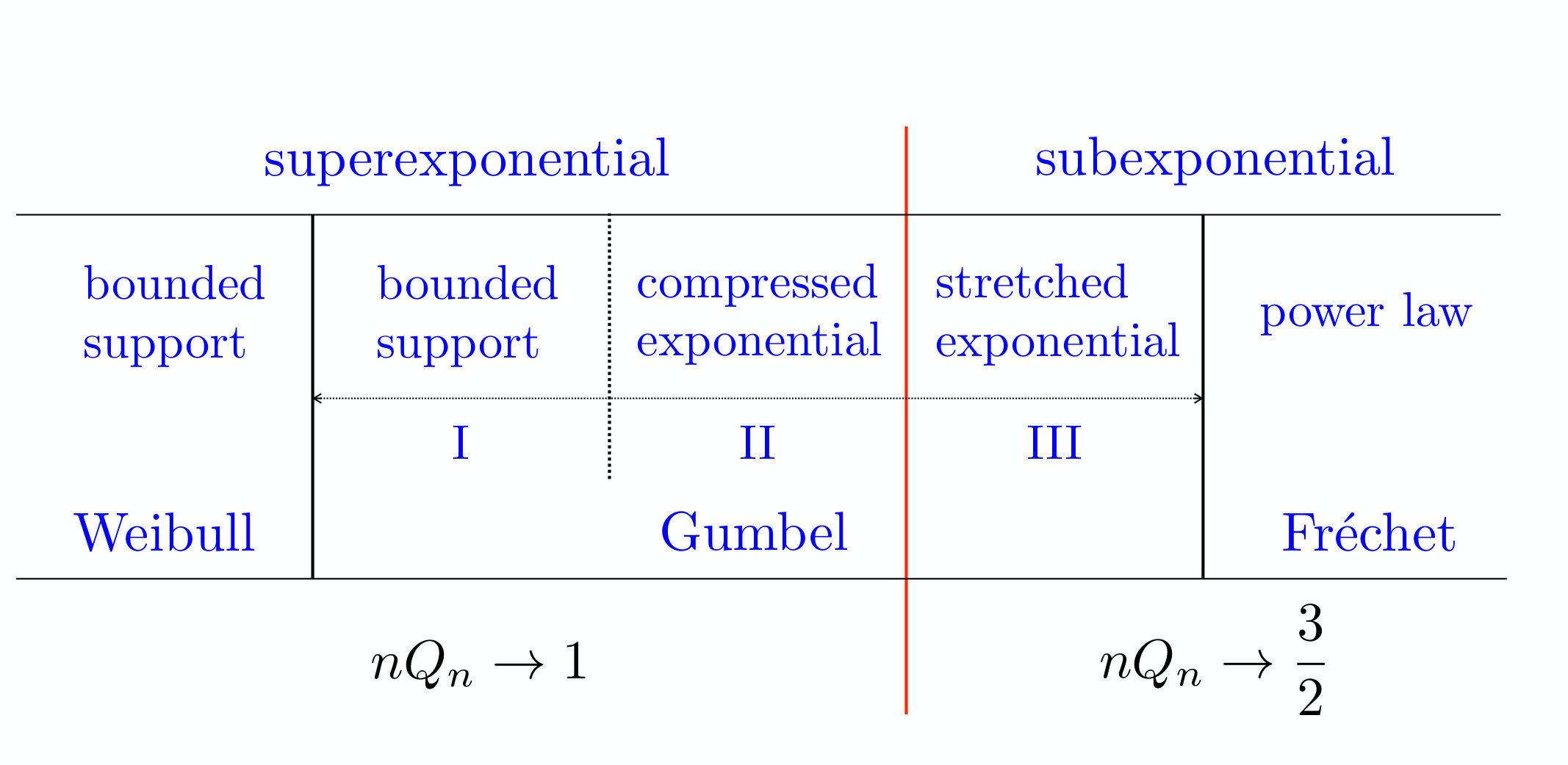 Figure 1
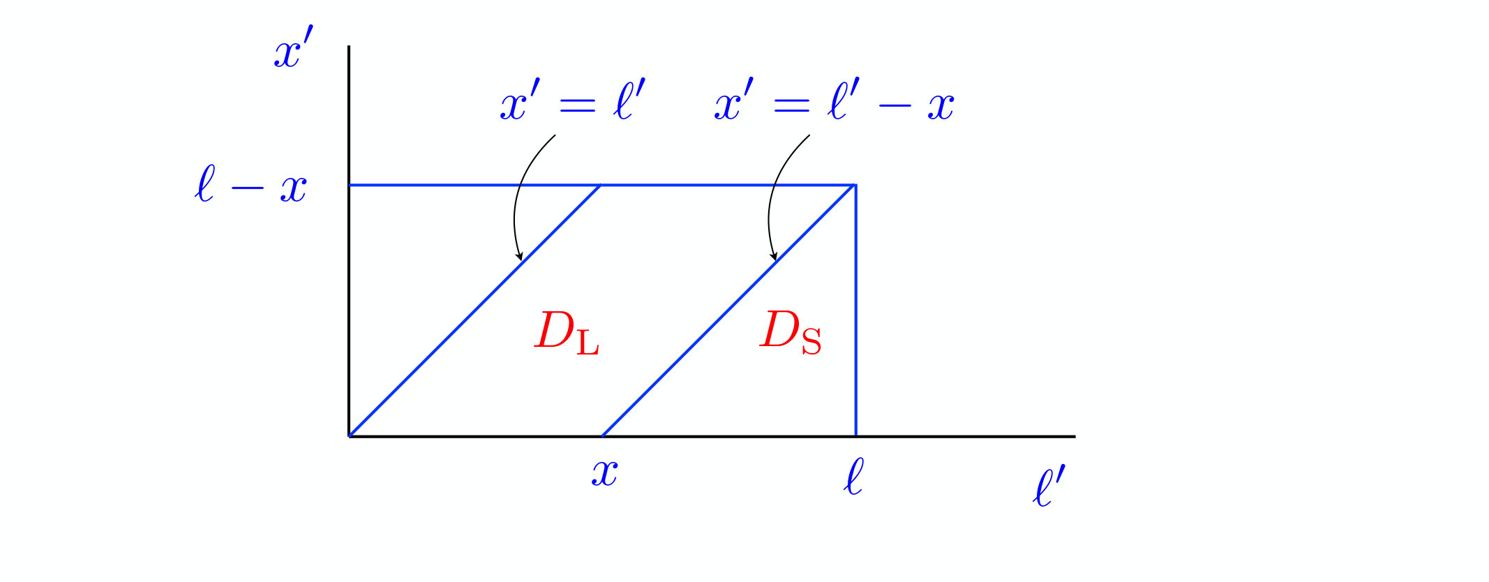 Figure 2
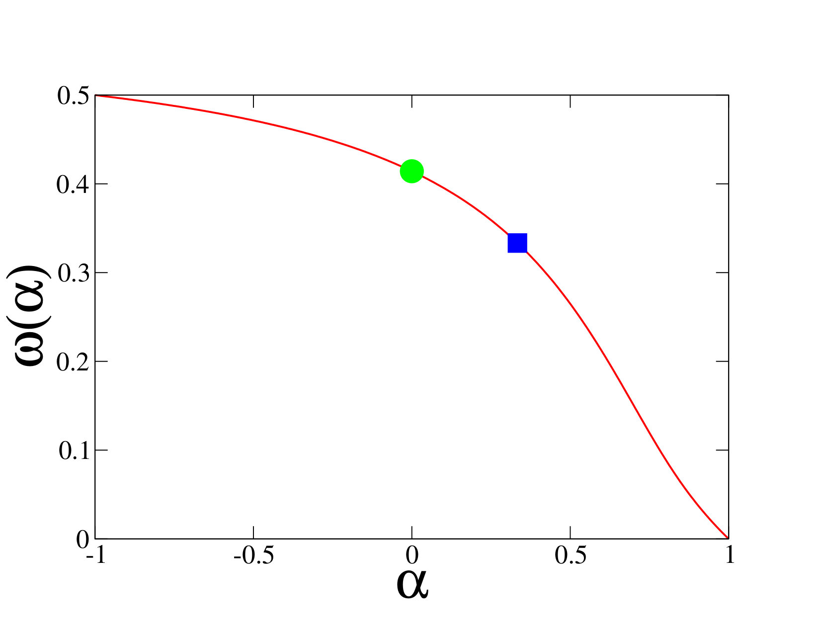 Figure 3
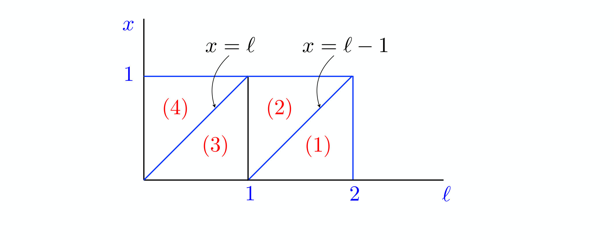 Figure 4
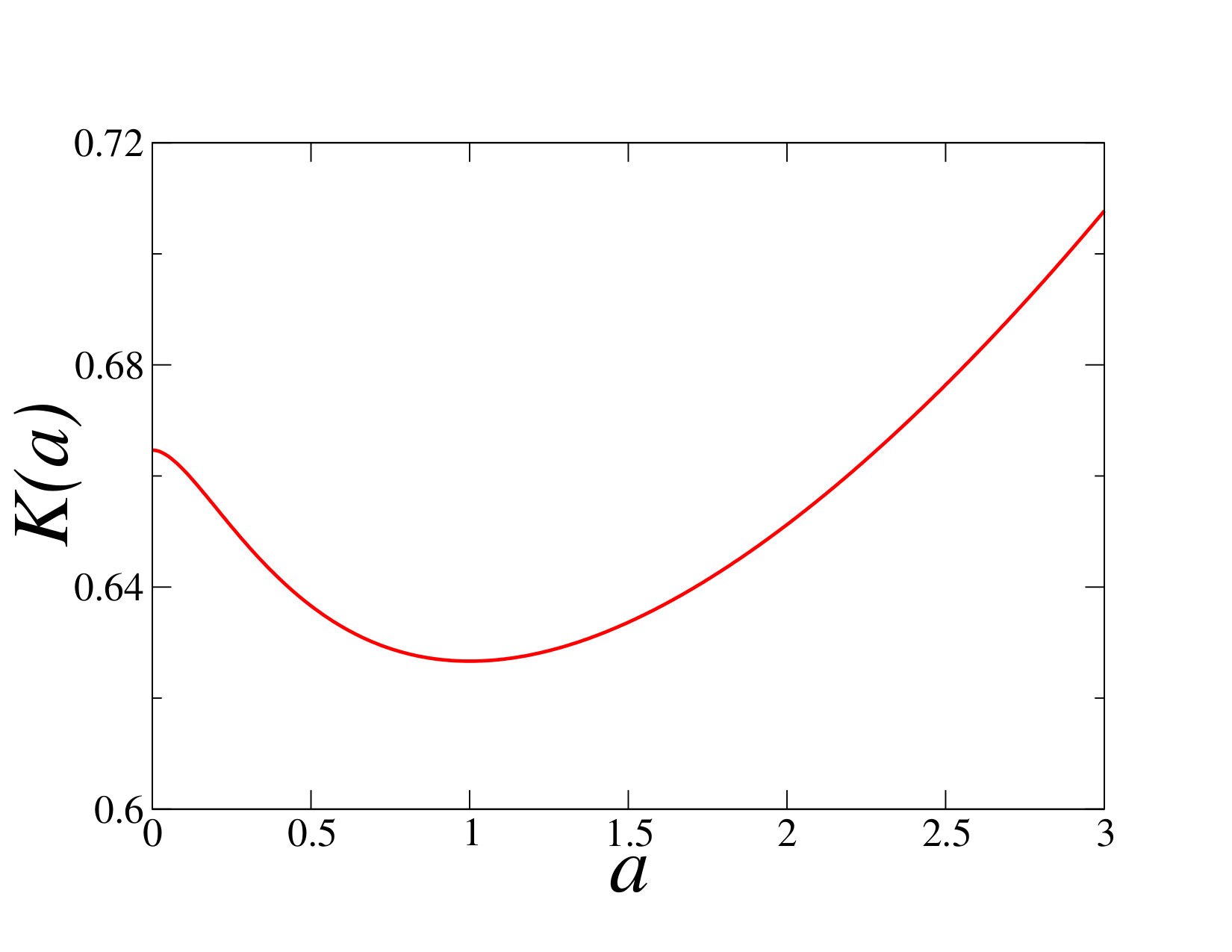 Figure 5
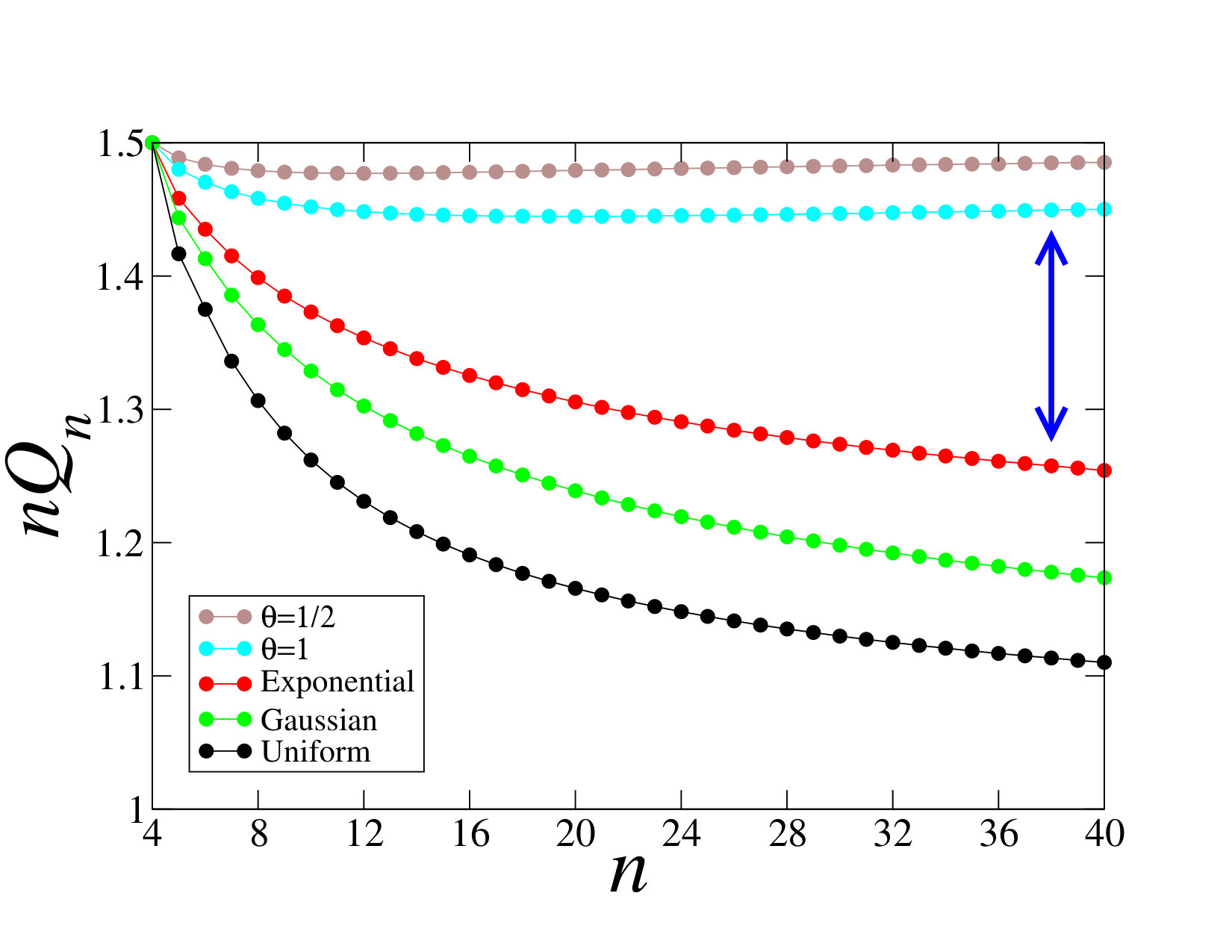 Figure 6
| Distribution | support | ||
|---|---|---|---|
| Uniform | |||
| Exponential | |||
| Half-Gaussian | |||
| Power-law () |
| 2 | 3 | 4 | 5 | 6 | 7 | 8 | |
|---|---|---|---|---|---|---|---|
| 1 | |||||||
| 1 |
| 2 | 3 | 4 | 5 | 6 | 7 | 8 | |
| 1 | |||||||
| 1 | |||||||
| 1 |
Peer Reviews
No public reviews on file for this paper yet. If you reviewed it on a platform where reviews are public (OpenReview, ICLR, NeurIPS, ICML), you can paste yours below so the community can read it here.
Videos
No videos yet. Explain this paper in a talk, walkthrough, or lecture? Add one.
Records for the moving average of a time series
Claude Godrèche and Jean-Marc Luck
Institut de Physique Théorique, Université Paris-Saclay, CEA and CNRS, 91191 Gif-sur-Yvette, France
Abstract
We investigate how the statistics of extremes and records is affected when taking the moving average over a window of width of a sequence of independent, identically distributed random variables. An asymptotic analysis of the general case, corroborated by exact results for three distributions (exponential, uniform, power-law with unit exponent), evidences a very robust dichotomy, irrespective of the window width, between superexponential and subexponential distributions. For superexponential distributions the statistics of records is asymptotically unchanged by taking the moving average, up to interesting distribution-dependent corrections to scaling. For subexponential distributions the probability of record breaking at late times is increased by a universal factor , depending only on the window width.
,
1 Introduction
When monitoring a time series, a feature which immediately attracts the attention of the observer is the sequence of record values, viz., the successive largest or smallest values in the series [1, 2, 3]. The first example which comes to mind are weather records, i.e., the extreme occurrences of weather phenomena such as the coldest or hottest days, the most rainy or windy days, and so on, for which studies abound (see [4, 5, 6, 7, 8, 9] and references therein). Other examples of records encountered in diverse complex physical systems are reviewed in [10], to which the reader is referred for a comprehensive list of references.
The simplest situation to analyse is when the data are samples of a sequence of independent, identically distributed (iid) random variables. In such an instance much is known on the statistics of records [1, 2, 3, 4, 11, 12], whose basics are easy to grasp. Consider a sequence of iid continuous random variables , with common distribution function and density . Throughout the following we assume that the are positive. A record is said to occur at step if is larger than all previous variables, i.e., if
[TABLE]
where denotes the largest amongst the first random variables. The probability of this event, or probability of record breaking,
[TABLE]
equals
[TABLE]
as a consequence of the fact that the random variables are exchangeable [2, 3]. The number of records up to time takes the values and can be expressed as the sum
[TABLE]
where the indicator variable is equal to 1 if is a record and to 0 otherwise. Taking the average, we have , and so
[TABLE]
where is the th harmonic number and is Euler’s constant. It is a simple matter to show that the indicator variables are statistically independent [2, 3, 10]. The distribution of ensues from this fact by elementary considerations (see also section 7.4 below). The simple expression (1.1) of the probability of record breaking and the full distribution of are universal, in the sense that they do not depend on the underlying distribution . From this standpoint the statistics of records for iid random variables exhibits a high degree of degeneracy. In contrast, the statistics of the extreme value is distribution dependent, as is well known [13].
In the present work we investigate the statistics of records for sequences made of sums of successive iid positive random variables, defined as follows. For ,
[TABLE]
for ,
[TABLE]
or more generally,
[TABLE]
The first terms of these sequences, which have not been written down explicitly, may be omitted in the analysis of records. For instance, in (1.4), is always smaller than . In (1.5), and are always smaller than , and so on.
Up to a normalisation, each of these sequences can be seen as the moving average of the sequence of iid variables , defined as the mean of the last terms. For instance the moving average with is
[TABLE]
Taking the moving average is a well-known method to analyse time series, which is equivalent to making a convolution of the signal by a square window, thus smoothing the signal. For instance, instead of looking at the daily temperature at a given location, one can take the moving average over a period of one week, corresponding to choosing . The question posed here amounts therefore to knowing how records are affected by taking such an average. The normalisation by the factor does not affect the outcome of the subsequent analysis.
Here the focus will be essentially on the particular case . Keeping the same notations as for the iid case, we shall primarily investigate the probability of record breaking,
[TABLE]
where denotes the largest amongst the first ones,
[TABLE]
and the mean number of records up to ,
[TABLE]
where records are counted from the first complete sum onwards. As we shall see, these quantities are now sensitive to the choice of the underlying distribution of the parent random variables . On the one hand, this does not come as a surprise since the new variables are no longer exchangeable, and the occurrences of records at various places are no longer independent. On the other hand, it is yet slightly paradoxical that the degeneracy induced by the exchangeability of the iid parent random variables is now removed, revealing features of their common distribution, since by taking the moving average one could have expected a loss of information instead. We shall also study some features of the distribution of .
In a nutshell, the main outcome of this work is as follows. We find that the product has only two possible limits for , depending on the class of distribution , namely
[TABLE]
for superexponential distributions, that is, distributions either having a bounded support or falling off faster than any exponential, whereas
[TABLE]
for subexponential distributions, whose tails decrease more slowly than any exponential. The pure exponential distribution belongs to the first class, albeit marginally. Figure 1 shows a plot of against for all the examples of probability distributions considered in the present paper (see table 1). Each dataset is the outcome of the numerical generation of sequences. The vertical arrow underlines that the dichotomy between (1.10) and (1.11) becomes more and more visible as increases. The values of for are universal, i.e., independent of the underlying distribution (see section 2.6).
For higher values of the window width , denoting the probability of record breaking by , (1.10) still holds for superexponential distributions, i.e.,
[TABLE]
while, for subexponential distributions, (1.11) becomes
[TABLE]
where the are universal rational numbers given by
[TABLE]
for , and obtained by means of the Sparre Andersen theorem.
The setup of this paper is as follows. Sections 2 to 6 concern the case . In section 2 we present the general setting which will be used in all subsequent exact or asymptotic developments. The next three sections are devoted to exact analytical solutions of the problem for three distributions: the exponential distribution (section 3), the uniform distribution (section 4), and the power-law distribution with index (section 5). In order to compare the probability of record breaking to its universal value in the iid situation (see (1.1)), we set
[TABLE]
The exponential distribution appears as a marginal case where (1.10) holds, albeit with a logarithmic correction
[TABLE]
For the uniform distribution falls off as
[TABLE]
whereas (1.11) holds for the power-law distribution with . A heuristic asymptotic analysis of the general case is then performed in section 6, where the dichotomy between (1.10) and (1.11) is explained in simple terms, and an estimate for the relative correction is derived. Higher values of the window width are considered in section 7 along the same line of thought. The overall picture, including the dichotomy between (1.10) and (1.11), remains unchanged. The non-trivial limit in (1.11) is replaced by the -dependent but otherwise universal limit (1.14). Section 8 contains a brief discussion of our findings.
Let us finally mention that the statistics of persistent events for the sequence (1.4) has been studied in [14, 15, 16], for the case where the parent variables have a symmetric distribution .
2 General setting
This section sets the basis of all subsequent exact or asymptotic developments. Hereafter and until the end of section 6 we focus our attention on the sequence (1.4) of sums of two terms. Higher values of the width will be considered in section 7.
2.1 Recursive structure
We start by highlighting the recursive structure of the problem. The first two maxima are necessarily and . The next maxima obey the recursion
[TABLE]
This recursion should be understood as follows. Starting from the couple of random variables , one draws the random variable , which is independent of and , and sets . This generates the new , or alternatively the new couple :
[TABLE]
In other words, at each time step , the newly drawn random variable acts as a noise on the dynamics of the couple . The value of depends on the branch of the recursion, denoted respectively by (for larger) and (for smaller):
[TABLE]
In the first case, is a record since it satisfies
[TABLE]
This event occurs with probability (see (1.7)). Hereafter we make use of the recursion (2.1) to derive the key relations (2.14) and (2.15) for the functions introduced in (2.3).
Let us mention that a similar, albeit simpler recursive scheme applies to the theory of records for iid random variables.
2.2 Basic quantities
Starting from the joint distribution function of the couple of random variables ,
[TABLE]
and taking its derivative with respect to , yields the quantity
[TABLE]
which plays a central role in the present work. It is equivalently defined as
[TABLE]
The underlying distribution is recovered in the limit:
[TABLE]
By differentiating with respect to , one gets the joint probability density of the couple :
[TABLE]
Conversely, integrating on the second variable restores
[TABLE]
In particular the distribution function of the maximum is obtained when the integral runs over its full range (i.e., ):
[TABLE]
Its derivative with respect to yields the density . The determination of the mean maximum ensues:
[TABLE]
Finally, the normalization of the joint density implies
[TABLE]
2.3 First values of
The quantities defined above have explicit expressions for and 2 in full generality.
For we have
[TABLE]
whenever , since . Differentiating with respect to gives
[TABLE]
and
[TABLE]
For , knowing that allows one to compute
[TABLE]
from which ensues by derivation with respect to :
[TABLE]
consistently with the definition (with informal notation)
[TABLE]
Then, taking a derivative with respect to , we have
[TABLE]
and finally
[TABLE]
2.4 Recursion relation for the function
The recursion (2.1) implies
[TABLE]
where denotes Heaviside function. The right-hand side of this equation decomposes into two contributions, associated to the two branches and ,
[TABLE]
where the domains and , depicted in figure 2, are respectively defined as
[TABLE]
hence
[TABLE]
Adding these two contributions yields
[TABLE]
which vanishes whenever its two arguments are equal ():
[TABLE]
We thus obtain the following recursion relation for the function :
[TABLE]
This equation and its differential form
[TABLE]
obtained by differentiating (2.14) with respect to 111Throughout the following, accents on functions denote their (partial) derivatives with respect to ., are key formulas of this work and the starting points of many subsequent developments.
As a consequence of (2.14), we have ()
[TABLE]
Finally, differentiating (2.10) with respect to yields
[TABLE]
with the notations
[TABLE]
using (2.11) and (2.12). Alternatively, differentiating (2.14) with respect to gives
[TABLE]
which is identical to (2.17).
2.5 Probability of record breaking
The probability of record breaking is the probability that the last variable is larger than all previous ones (see (1.7)),
[TABLE]
This probability thus equals the weight of branch . For, recalling (2.6) and (2.17),
[TABLE]
where the two terms corresponding respectively to the weights of the two branches and are and . So the expression of is ()
[TABLE]
2.6 Universal values of the probability of record breaking
The first few values of are universal, i.e., independent of the underlying distribution . For ,
[TABLE]
since is always larger that . This result can be recovered by inserting (2.7) into (2.21). For ,
[TABLE]
since is equivalent to , which holds with probability . This result can be recovered by inserting (2.8) into (2.21). It turns out that for , has also a universal value,
[TABLE]
irrespective of the distribution . This can be demonstrated by a simple application of the Sparre Andersen theorem [17, 18, 19]. This theorem states in particular that, for a sequence of iid variables with a continuous symmetric distribution, the probability that the first partial sums are all positive,
[TABLE]
is a universal rational number,
[TABLE]
for , with generating function
[TABLE]
In the present case, by definition,
[TABLE]
where the random variables and are iid and have a continuous symmetric distribution. Therefore the theorem applies and , which is the result announced in (2.24). It would be cumbersome to recover this directly by means of (2.21).
The probability of record breaking is no longer universal for . It is indeed clear from figure 1 that already depends on the underlying distribution .
It results from the foregoing that the first values of the mean number of records (see (1.9))
[TABLE]
are also universal.
In the forthcoming sections we apply the general formalism presented in this section to derive analytical solutions of the differential recursion (2.15) for the exponential distribution (section 3), the uniform distribution (section 4), and the power-law distribution with index (section 5).
3 Exponential distribution
This section presents an exact solution of the problem for the case of exponentially distributed random variables , with common density and distribution function (see table 1).
3.1 Differential equations
The exact solutions derived in this section and in the two subsequent ones rely on the differential equation (2.15), which reads, in the present case,
[TABLE]
Differentiating once more yields ()
[TABLE]
This is a recursive differential equation in the variable , while plays the role of a parameter. Setting in (3.1) gives ()
[TABLE]
where the interpretation of the first term is given in (2.16).
3.2 First values of
For the first few values of , we obtain
[TABLE]
[TABLE]
Inserting these expressions into (2.21), we recover the universal results for , and derived in section 2.6. Equations (2.13) and (3.3) are complemented by
[TABLE]
We have also
[TABLE]
[TABLE]
Inserting these expressions into (2.5) yields , and .
3.3 Generating function
In order to solve the recursive differential equation (3.2) for all values of , we introduce the generating function
[TABLE]
which satisfies (using (3.2))
[TABLE]
the solution of which is
[TABLE]
with
[TABLE]
The amplitudes are determined by the boundary conditions (see (3.2))
[TABLE]
yielding
[TABLE]
3.4 Probability of record breaking
Using (2.21), the generating function of the reads
[TABLE]
with
[TABLE]
and
[TABLE]
The integral over in (3.7) cannot be carried out in closed form. By expanding as a power series in and integrating term by term with respect to , we obtain the values of the probability of record breaking and mean number of records given in table 2 up to .
The asymptotic decay of at large can be derived as follows. Setting , (3.8) becomes
[TABLE]
in the relevant regime where and are simultaneously small. Inserting this into (3.7), and dealing with as a continuous variable, we obtain the estimate
[TABLE]
Performing the inverse Laplace transform yields
[TABLE]
Setting
[TABLE]
and changing integration variable from to such that , we obtain formally
[TABLE]
The expression underlined by the brace is the normalized Gumbel distribution with parameter . This distribution is peaked around . More precisely, considering the following average with respect to this distribution,
[TABLE]
we obtain
[TABLE]
for any slowly varying function , where is Euler’s constant. Applying this to the function inside the large parentheses in (3.11), we obtain the expansion
[TABLE]
with the notation (3.10) and
[TABLE]
Omitting details, let us mention that a similar analysis yields the following expansion for the mean number of records up to time :
[TABLE]
Equations (3.12) and (3.13) give the first few terms of asymptotic expansions to all orders in . The ambiguity in the formal expression (3.11) originating in the pole at , i.e., , is indeed exponentially small in .
3.5 Mean value of the maximum
Using (2.5), (2.16) and (3.5), we obtain the generating function of the mean value of the largest variable up to time ,
[TABLE]
The explicit expression (3.6) of the generating function implies
[TABLE]
so that
[TABLE]
and finally
[TABLE]
This remarkable identity between mean values is a peculiarity of the exponential distribution. The first few values of can therefore be read from table 2, whereas its asymptotic growth can be read from (3.13). Let us notice that a similar identity, i.e., , holds for extremes and records of exponentially distributed iid random variables (see [20, 21] for a discussion of related matters).
4 Uniform distribution
The case where the random variables are uniformly distributed on [0, 1], with common density and distribution function for (see table 1), also lends itself to an exact solution of the problem.
4.1 Sectors
Here, the relevant part of the plane is the rectangle defined by and . This region splits into four sectors (see figure 3):
[TABLE]
The functions assume a priori different analytical forms in these four sectors. The recursion (2.14) reads
[TABLE]
The first function is independent of , whereas the last one vanishes, so the information of interest is contained in sectors (2) and (3).
The probability of record breaking reads
[TABLE]
with
[TABLE]
Similarly, the mean value of the maximum reads
[TABLE]
with
[TABLE]
Finally, differentiating (4.1) with respect to , we obtain the following differential equations, valid in both sectors and :
[TABLE]
These equations, which can alternatively be read off from (2.15), will be instrumental hereafter. We thus obtain the following expressions for the first values of :
[TABLE]
for ,
[TABLE]
for , and
[TABLE]
for .
4.2 Analysis of sector (3)
The generating function
[TABLE]
satisfies
[TABLE]
because of (4.2),
[TABLE]
because of (4.3), and
[TABLE]
because of (2.13). Hence
[TABLE]
where the amplitudes and , which depend a priori on and , are determined by the boundary conditions (4.4). We thus obtain
[TABLE]
Hence
[TABLE]
and
[TABLE]
Relationship with Euler numbers. Consider positive numbers such that for . These conditions define a volume for every integer . The generating function of these numbers reads [22]
[TABLE]
We have
[TABLE]
where are the Euler numbers, listed as sequence number A000111 in the On-Line Encyclopedia of Integer Sequences [23]. The volumes are also simply related to the , as we now show. Let us note (see (4.6)) that
[TABLE]
hence, for ,
[TABLE]
The relationship between the two sequences and comes from the fact that
[TABLE]
hence, integrating over ,
[TABLE]
Let us remark that
[TABLE]
Finally, the generating function has a pole at , with residue 2, and therefore
[TABLE]
4.3 Analysis of sector (2)
The generating function
[TABLE]
satisfies
[TABLE]
because of (4.2),
[TABLE]
because of (4.3), and
[TABLE]
as a consequence of (4.1), using the fact that is independent of .
We thus obtain, in analogy with (4.5)
[TABLE]
with
[TABLE]
We have therefore
[TABLE]
and
[TABLE]
At variance with (4.6) and (4.7), the integrals over in (4.9) and (4.10) cannot be carried out in closed form.
4.4 Results
By expanding the integrands of (4.9) and (4.10) as power series in , integrating over term by term, and adding up the contributions of (4.6) and (4.7), we obtain exact rational expressions for the probability of record breaking , the mean number of records and the mean value of the maximum . These outcomes are given in table 3 up to .
The asymptotic behavior at large of the various quantities of interest can be derived as follows. First of all, the contribution of sector (3) is exponentially small, and therefore entirely negligible. Setting again , the integrals entering (4.9) and (4.10) are dominated by a range of values of the difference that shrinks proportionally to as . Changing integration variable from to such that , and keeping only terms which are singular in , we obtain
[TABLE]
and so
[TABLE]
and
[TABLE]
Finally, omitting details, we obtain a similar asymptotic expansion for the mean number of records, i.e.,
[TABLE]
where the finite part reads
[TABLE]
5 Power-law distribution with index
The case where the random variables have a power-law distribution with index , with common density and distribution function for (see table 1), is our last example giving rise to an exact solution of the problem, although end results are somewhat less explicit than in the two previous cases. The distribution under consideration is marginal, in the sense that is logarithmically divergent.
5.1 Differential equations
In the present case, the key equation (2.15) reads
[TABLE]
for , , and . Setting
[TABLE]
the new functions obey the differential equation
[TABLE]
with boundary condition , as well as
[TABLE]
We thus obtain
[TABLE]
5.2 Generating function
In order to solve the recursive differential equations (5.2), (5.3), we introduce the generating function
[TABLE]
which obeys
[TABLE]
with boundary condition
[TABLE]
as well as
[TABLE]
The general solution to (5.7) reads
[TABLE]
with
[TABLE]
Notice the similarity with (3.6). The amplitudes are determined by (5.5) and (5.6), yielding
[TABLE]
This result demonstrates that the functions only involve integer powers of and , besides rational functions.
5.3 Probability of record breaking
The generating function of the reads
[TABLE]
by virtue of (2.21), (5.1) and (5.4), where is given by (5.8). The integral over can be carried out in closed form. We thus obtain
[TABLE]
with
[TABLE]
and
[TABLE]
As was the case for (3.7) and (4.9), the integrals over in (5.9) cannot be carried out analytically in closed form. By expanding the integrand in (5.9) as a power series in and integrating term by term with respect to , we obtain the following values for the probability of record breaking , besides the universal ones derived in section 2.6:
[TABLE]
and so on. In contrast with the two previous exactly solvable cases (see tables 2 and 3), here the non-universal are not rational, and they involve the values of Riemann zeta function at larger and larger positive integers.
The asymptotic behavior of at large can be derived from (5.9) by setting again , and considering the regime where and are simultaneously small. To leading order, (5.9) reduces to
[TABLE]
i.e., performing the inverse Laplace transform,
[TABLE]
up to negligible boundary terms. The above result is an explicit instance where (1.11) holds. A full asymptotic expansion of can be derived by keeping track of higher orders, yielding
[TABLE]
Finally, omitting details, we obtain a similar asymptotic expansion for the mean number of records, i.e.,
[TABLE]
where the finite part reads
[TABLE]
5.4 Distribution of the maximum
Here is divergent, so that it makes no sense to evaluate . The full distribution of should be considered instead. We have
[TABLE]
as a consequence of (2.4), (2.14) and (5.1). We thus obtain
[TABLE]
The corresponding generating function reads
[TABLE]
where the last expression is a consequence of (5.8).
The scaling behavior of the distribution of at large can be derived along the lines of the previous section. To leading order, we find the simple result
[TABLE]
In particular, the median value , such that , reads
[TABLE]
The full asymptotic expansion of in the regime where and are comparable reads
[TABLE]
and so
[TABLE]
6 Asymptotic analysis of the general case
The probability of record breaking exhibits a great variety of asymptotic behaviors, depending on the underlying distribution . This is exemplified by the three exactly solvable cases studied in sections 3 to 5. In terms of the correction such that (see (1.15)), we have seen that
[TABLE]
for the exponential distribution (see (3.12)),
[TABLE]
for the uniform distribution (see (4.11)), and
[TABLE]
which is equivalent to (1.11), for the power-law distribution with (see (5.10)).
This section is devoted to a heuristic but systematic analysis of the dependence of the asymptotic behavior of on the underlying distribution . It will turn out that the exponential distribution, where falls off logarithmically (see (6.1)), is a marginal case. For superexponential distributions, the analysis of sections 6.3 and 6.4 demonstrates that falls off to zero and yields a general asymptotic formula for (see (6.10)). For subexponential distributions, it will be shown in section 6.5 that and go to the universal limits (1.11) and (6.2). This dichotomy will be extended to higher values of the window width in section 7.
6.1 Cyclization of the sequence
The first step of the analysis consists in comparing the problem at hand with a cyclic variant of it. For the former, we have
[TABLE]
with
[TABLE]
(see (1.7) and (1.8)). The cyclic variant of the problem is defined by introducing
[TABLE]
The sequence thus obtained involves the basic variables in a cyclically invariant fashion. It has therefore exchangeable entries, and so
[TABLE]
Introducing the events
[TABLE]
we have
[TABLE]
and so
[TABLE]
This equation gives a description of the difference in terms of a conditional probability, which will prove useful in the following.
6.2 Decoupled model
We now consider a decoupled variant of the original problem, whose main advantage is that the expression (6.3) can be given the explicit form (6.9), which will in turn yield the estimate (6.10) for the correction in appropriate situations.
The decoupled model is defined as follows. The random variables of the original problem are replaced by a sequence of iid random variables
[TABLE]
where and are two independent replicas of the original random variables with common density and distribution function . The number of variables is therefore doubled with respect to the original problem. The distribution function and the density of the variables thus read
[TABLE]
In terms of the Laplace transform
[TABLE]
this reads
[TABLE]
The conditional density of given , denoted by , is equal to
[TABLE]
The largest among the first variables , denoted by
[TABLE]
has distribution function
[TABLE]
and density
[TABLE]
Using (6.7) and (6.8), the density of is
[TABLE]
Within the setting of the decoupled model, the conditional probability introduced in (6.3) therefore reads
[TABLE]
with
[TABLE]
When is large, the factor in (6.9) selects large values of , such that scales as . These are the typical values of . The product underlined by the brace, which already entered (6.2) and (6.7), describes to what extent the distribution of is affected by the conditioning by such a large value of the sum .
6.3 The key dichotomy
The dichotomy between the two limits (1.10) and (1.11) is now shown in general albeit non-rigorous terms to be dictated by the form of the tail of the underlying parent distribution or, equivalently, by the analytic structure of its Laplace transform .
For superexponential distributions, i.e., distributions either having a bounded support or falling off faster than any exponential, such as e.g. a half-Gaussian or any other compressed exponential, is an entire function, i.e., it is analytic in the whole complex -plane. Then, as a general rule, (see (6.2)) has a slower decay than . Furthermore, if the sum is atypically large, then both and are atypically large as well, with very high probability. As a consequence, the conditional probability , as given by (6.9), falls off to zero for large . Simplifying the latter expression, we thus obtain the following asymptotic estimate for :
[TABLE]
We claim that this prediction becomes asymptotically exact for all superexponential distributions, in the sense that it correctly describes the decay of , to leading order for large , in spite of its heuristic derivation using the decoupled model. The rationale behind this claim is that the difference between the original and the decoupled models, measured by the relative difference between and , is consistently found to decay to zero, proportionally to the estimate (6.10) for . 2.
For subexponential distributions, i.e., distributions which fall off smoothly enough and less rapidly than any exponential, such as e.g. a power law or a stretched exponential, has an isolated branch-point singularity at . The asymptotic equivalence of the tails,
[TABLE]
can be derived by an inverse Laplace transform of (6.6), where the contour integral is dominated by the singularity of at . Equation (6.11) may be used as a mathematically rigorous definition of the class of subexponential distributions, following Chistyakov [24]. Its intuitive meaning is the following: if the sum is very large, then one of the terms, either or —hence the factor 2—is typical, i.e., distributed according to , while the other one is essentially equal to . This behavior underlies the phenomenon of condensation for subexponential random variables conditioned by an atypical value of their sum (see [25] for a recent review and the references therein). As a consequence of (6.11), for subexponential distributions , the estimate (6.9) remains of order unity for large . The decoupled model is therefore of little use to understand the original one. This situation will be investigated in section 6.5, where and will be shown to admit the universal limits (1.11) and (6.2).
For exponential distributions, i.e., distributions falling off either as a pure exponential , with , or as the product of such an exponential by a more slowly varying prefactor, such as e.g. a power of , the leading (i.e., rightmost) singularity of is located on the negative real axis at . For our purpose, these distributions are marginal since they can lie on either sides of the dichotomy between (1.10) and (1.11) (see section 6.4.2).
6.4 Superexponential and (some) exponential distributions
The prediction (6.10) is now made explicit for a variety of superexponential and exponential distributions .
6.4.1 Pure exponential distribution.
This is the distribution for which an exact solution has been presented in section 3. We have
[TABLE]
The estimate (6.10) therefore reads
[TABLE]
This integral can be evaluated in analogy with (3.9). Setting (see (3.10)) and , we obtain
[TABLE]
hence
[TABLE]
A comparison with the exact expansion (3.12) shows that the estimate (6.10) is correct to leading order in this marginal case. The difference between the estimate (6.13) and the exact result is indeed subleading, since it scales as .
6.4.2 Exponential distribution modulated by a power law.
We now consider distributions falling off as an exponential modulated by a power law, i.e.,
[TABLE]
where is arbitrary (positive or negative).
Let us consider first the case where . We have then
[TABLE]
and
[TABLE]
with . Performing the integrals entering (6.10), we obtain
[TABLE]
This integral can be evaluated in analogy with (3.9). Setting and , we obtain formally
[TABLE]
To leading order, the identification yields the estimate
[TABLE]
We are thus led to claim that exponential distributions of the form (6.14) with , and presumably all exponential distributions such that as the leading singularity is approached from the right (), belong to the superexponential side of the dichotomy, in the sense that (1.10) holds, and that (6.16) correctly predicts the decay of the correction . The logarithmically slow fall off of the latter expression confirms the marginal character of this class of exponential distributions.
On the contrary, if the exponent entering (6.14) is negative, the above derivation already breaks down at the level of (6.15). Exponential distributions of the form (6.14) with , and presumably all exponential distributions such that remains bounded as , therefore share with subexponential distributions the property that the estimate does not decay to zero, with the expected consequence that (1.11) should hold.
6.4.3 Distributions with bounded support and power-law singularity.
We now consider the case where is supported by the interval [0, 1] and has a power-law singularity at its upper edge, i.e.,
[TABLE]
with the notations , . The exponent and the amplitude are arbitrary. We have . Performing the integrals entering (6.10), we obtain a universal decay for , irrespective of the exponent , i.e.,
[TABLE]
where the amplitude reads
[TABLE]
The amplitude is shown in figure 4. It has a local maximum at and a local minimum at The latter value agrees with the exact result (4.11) for the uniform distribution. This provides another corroboration of our claim that the estimate (6.10) is correct to leading order. The exponential growth of the amplitude at large suggests that the decay ceases to hold for distributions with an infinitely large exponent, i.e., with an essential singularity at their upper edge.
6.4.4 Distributions with bounded support and exponential singularity.
We now consider the case where is supported by the interval [0, 1] and has an exponentially small singularity at its upper edge, of the form
[TABLE]
with . Using the same notations as above, and working within exponential accuracy, we have
[TABLE]
for small , where the integral is dominated by a saddle point at , so that
[TABLE]
Similarly, the -integral entering (6.10) is dominated by a saddle point at , with , and so
[TABLE]
Using once more the saddle-point method, we obtain a power-law decay of the form
[TABLE]
where the exponent
[TABLE]
decreases monotonically as a function of , from to .
6.4.5 Compressed exponential distributions.
We now consider the case where has a compressed exponential (or superexponential) tail extending up to infinity, of the form
[TABLE]
with . The analysis of this case is very similar to the previous one. We have
[TABLE]
for large , where the integral is dominated by a saddle point at , so that
[TABLE]
Similarly, the -integral entering (6.10) is dominated by a saddle point at , with , and so
[TABLE]
We thus obtain a power-law decay of the form
[TABLE]
where the exponent
[TABLE]
increases monotonically as a function of , from as to . In particular, for the half-Gaussian distribution (), we predict the decay exponent
[TABLE]
As it turns out, the decay exponents (see (6.21)) and (see (6.23)) can be unified into a single function
[TABLE]
of a parameter in the range , as shown in figure 5. Distributions with a bounded support and an exponential singularity with index correspond to , whereas compressed exponential distributions with index correspond to , with the identifications
[TABLE]
The exponent is a decreasing function from to , via the common limiting value , characteristic of distributions with a double exponential fall-off, either at the upper edge of a compact support or at infinity.
6.5 Subexponential distributions
We now consider subexponential distributions, whose tails decrease more slowly than any exponential. Our goal is to show that the correction goes to the universal limit (6.2), i.e., that falls off as
[TABLE]
for large . This result agrees to leading order with the expansion (5.10), ensuing from an exact solution for the power-law distribution with . It also agrees with the exact expression (6.33) of for finite in the limiting situation of exponentially broad distributions.
The gist of the derivation of (6.27) consists in looking for a solution to the integral recursion (2.14) in an approximately factorized form, i.e.,
[TABLE]
The condition (2.13) yields
[TABLE]
whereas is assumed to be small in the regime of interest where and are simultaneously large, with being kept finite. We set
[TABLE]
fixing thus the prefactor unambiguously. To leading order, the differential equation (2.15) yields
[TABLE]
Equation (6.31), with boundary conditions (6.29) and (6.30), admits a similarity solution where and the ratio are independent of , namely
[TABLE]
Whenever and are simultaneously large, (6.28) simplifies to
[TABLE]
so that (2.21) yields the estimate
[TABLE]
The analysis of this expression for large is somewhat similar to that of (6.9), performed in section 6.4. The exponential factor selects large values of , such that scales as . These are the typical values of . The subexponentiality of , in the intuitive sense explained below (6.11), suggests that the integral over the variable in (6.32) is dominated by the vicinity of its endpoints, i.e., of the regimes where either or the difference is kept finite. Adding these two contributions yields
[TABLE]
for large. Inserting this estimate into (6.32) leads to the announced result (6.27).
The statistics of the number of records for subexponential underlying distributions will be investigated at the end of section 7.4.
6.6 Exponentially broad distributions
We now consider the limiting class of exponentially broad distributions, defined by setting
[TABLE]
where is parametrically large, whereas has a fixed given distribution . Exponentially broad distributions play a part in the study of strongly disordered systems (see [26, 27] and the references therein). An explicit example is provided by the power-law distribution (see table 1) in the limit where the index goes to zero, with the identification and . The overwhelming simplification brought by exponentially broad distributions in the limit is that is equivalent to . In other words, the distribution is so broad that, if two independent variables and are drawn from the latter, one is negligible with respect to the other with very high probability.
Considering exponentially broad distributions in the limit is useful for our purpose in several regards. First, the exact probability of record breaking can be derived in this limit, even for finite . Second, as we shall see, the derivation gives an insight on the clustering of records underlying the non-trivial limit (1.11). Third, this approach will be readily extended to higher values of the window width in section 7, where other techniques are not available any more.
Within this setting, it is easy to derive the probability of record breaking . We recall that is the probability of having , with
[TABLE]
and so on. If the variables are drawn from an exponentially broad distribution, only two events contribute to :
The largest of the first -variables is . This occurs with probability . In the limit, the variable is also larger than all previous ones with certainty. Hence the contribution to . 2.
The largest of the first -variables is . This again occurs with probability . The condition reduces to , so that the relative probability of that event is . Hence the contribution to .
As a consequence, the probability of record breaking is exactly given by
[TABLE]
for all and all exponentially broad distributions in the limit.
The formula (6.33) gives both the exact value of for exponentially broad distributions and its asymptotic decay law (see (1.11), (6.27)) for all distributions with a subexponential tail. The above derivation also demonstrates that the excess in the probability of record breaking (6.33) with respect to the iid situation is due to a clustering of records. The second event of the above list indeed yields two consecutive records. Finally, the data shown in figure 1 suggest that (6.33) provides an absolute upper bound for . It is indeed quite plausible that the quantity plotted in figure 1 converges to the constant from below in the limit, uniformly in .
7 Extension to higher values of
In this last section we consider sequences (1.6) obtained by taking the moving average of a sequence of iid variables over an arbitrary finite window width . We shall mainly focus on the behavior of the probability of record breaking, that we now denote by
[TABLE]
The recursive structure of the problem described in section 2 still holds true, however it becomes somewhat inefficient, as the number of variables is higher. The recursion equation generalizing (2.14) indeed involves a multiple integral over variables. In particular, no exact solution is available any more. In spite of this, we shall be able to extend to higher values of most results of interest derived so far for .
7.1 Universal values of the probability of record breaking
The first few values of are universal, i.e., independent of the underlying distribution . Their values can be derived along the lines of reasoning of section 2.6, using again the Sparre Andersen theorem. The first case of interest is , where
[TABLE]
There is indeed always a record at , as is the first complete sum of terms. For , we have
[TABLE]
For , we have
[TABLE]
using the same argument as in section 2.6 for the derivation of for . More generally, for , with , we have
[TABLE]
where the expression of is given in (2.25).
The above formula generalizes the results of section 2.6 to an arbitrary window width . It exhausts the list of all universal values of the probability of record breaking. In other words, is the first non-universal one, just as for .
7.2 Superexponential and (some) exponential distributions
The explanation given in section 6.3 of the key dichotomy between (1.10) and (1.11), based on the analytic structure of the Laplace transform , is not limited to . Its consequences are therefore expected to hold irrespective of the window width .
For superexponential distributions, as well as for some exponentially decaying distributions, we are therefore again led to compare the original problem to its cyclic variant and to introduce a decoupled model, where the random variables of the original problem are now replaced by a sequence of iid random variables
[TABLE]
generalizing (6.4). If the sum is atypically large, then all its terms are atypically large as well, with very high probability. We therefore predict a behavior of type (1.10), i.e.,
[TABLE]
with the following estimate for the small relative correction :
[TABLE]
which is a direct generalization of (6.10). We again claim that this prediction is asymptotically correct, to leading order for large , whenever it decays to zero, i.e., essentially for all superexponential distributions.
The estimate (7.5) is now made explicit for a variety of distributions .
7.2.1 Pure exponential distribution.
For an exponential distribution with density and distribution function , we have
[TABLE]
as well as , to leading order for , and so (7.5) reads
[TABLE]
This integral can be evaluated along the lines of (3.9) and (6.12). Omitting details, we obtain to leading order
[TABLE]
This estimate vanishes identically for and coincides with (6.13) for . It demonstrates that the marginal character of the exponential distribution, with its logarithmic correction term, persists to all higher values of .
7.2.2 Exponential distribution modulated by a power law.
We now consider distributions falling off as an exponential modulated by a power law, i.e.,
[TABLE]
Along the lines of section 6.4.2, let us consider first the case where . We have
[TABLE]
with . Performing the integrals entering (7.5), we are left with the estimate
[TABLE]
This formula is a direct generalization of (6.16). We thus conclude that exponential distributions of the form (7.6) with belong to the superexponential side of the dichotomy, in the sense that (1.12) holds, with a correction falling off as (7.7). On the other hand, along the lines of section 6.4.2, we are led to claim that exponential distributions with lead to (1.13), just as subexponential distributions.
7.2.3 Distributions with bounded support and power-law singularity.
In the case where is supported by the interval [0, 1] and has a power-law singularity of the form (6.4.3) at its upper edge, we have
[TABLE]
with and . Performing the integrals entering (7.5), we obtain a power-law decay for , i.e.,
[TABLE]
where the exponent only depends on the width , whereas the amplitude reads
[TABLE]
This result extends (6.19) to higher values of . The amplitude has a local maximum for , a local minimum for , and grows exponentially fast at large . All these features hold irrespective of , and survive in the formal limit, i.e.,
[TABLE]
7.2.4 Distributions with exponential singularities.
To close, we consider distributions with a bounded support and an exponentially small singularity at their upper edge, of the form (6.20), as well as compressed distributions with a superexponential tail extending up to infinity, of the form (6.22).
We again obtain a power-law decay for the correction , with continuously varying decay exponents and , which can be unified into a single monotonically decreasing function
[TABLE]
of the parameter in the range , with the identifications (6.26). We have in particular , ensuring a smooth crossover with (7.8), for the limiting situation of distributions with a double exponential fall-off, and , corresponding e.g. to the half-Gaussian distribution.
7.3 Exponentially broad distributions
For exponentially broad distributions in the limit, the expression of can be derived along the lines of section 6.6. We recall that is the probability of having , with
[TABLE]
and so on. If the -variables are drawn from an exponentially broad distribution, only the following events contribute to :
The largest of the first -variables is . This occurs with probability . In the limit, the variable is also larger than all previous ones with certainty. Hence the contribution to . 2.
The largest of the first -variables is . This again occurs with probability . The condition reduces to , so that the relative probability of that event is . Hence the contribution to . 3.
The largest of the first -variables is . This again occurs with probability . The condition reduces to
[TABLE]
so that the relative probability of that event is , again by virtue of the Sparre Andersen theorem. Hence the contribution to , and so on.
Summing up the probabilities of the events listed above, we predict that the probability of record breaking is exactly given by
[TABLE]
for all and and all exponentially broad distributions in the limit. The numerator of the above formula reads
[TABLE]
where the integer numbers the items of the above list and where the expression of is given in (2.25). Equation (2.26) yields
[TABLE]
The are therefore universal rational numbers given by
[TABLE]
for , and growing as
[TABLE]
at large .
The formulas (7.4) and (7.9) overlap for two values of , namely and , for which they consistently predict
[TABLE]
7.4 Subexponential distributions
Following the line of thought sketched in the very beginning of section 7.2, we are led to extend the dichotomy between (1.10) and (1.11) to higher values of , and to predict the following asymptotic decay of the probability of record breaking at large :
[TABLE]
for all and all subexponential distributions , where the amplitude is predicted by the exact analysis of the limiting case of exponentially broad distributions (see section 7.3). The latter amplitude, given by (7.10), is therefore universal, in the sense that it only depends on the window width .
The formula (7.9) therefore has the same status as (6.33). It gives the exact value of for exponentially broad distributions in the limit for all . It is also expected to describe the asymptotic decay law of for all subexponential distributions, and furthermore to provide an absolute upper bound for for all .
8 Discussion
This paper was devoted to the statistics of records for the moving average of a sequence of iid variables. Most results concern the case where the window width is . The main emphasis has been put on the probability of record breaking at time , and on the distribution of the number of records up to time . In sections 3 to 5 we have given full analytical solutions of the problem for three particular parent distributions: exponential, uniform and power-law with . The exact results obtained there provide useful checks of the heuristic approach used in the asymptotic analysis of the general situation (section 6) and in its extension to higher values of (section 7).
Quite serendipitously, the three distributions which have lent themselves to an exact analytical treatment are prototypical in several regards. First, each of them is a representative of one of the three universality classes of extreme value statistics: Weibull, Gumbel and Fréchet. Second, they are also representatives of the dichotomy, as regards the properties of records for the moving average, between superexponential distributions, where the product tends to unity and the distribution of the number of records is asymptotically Poissonian, and subexponential distributions, where admits the non-trivial universal limit 3/2, or more generally , and the distribution of the number of records exhibits novel universal clustering features. The uniform and power-law distributions are respectively typical of the superexponential and subexponential classes, whereas the exponential distribution is a representative of the exponential class, which is marginal and split on both sides of the dichotomy, as seen in section 6.4.2.
Our main results can be summarized in the sketchy representation of the realm of parent probability distributions shown in figure 6. The tail of the distribution is more and more heavy, i.e., the density falls off more and more slowly, as one progresses from left to right. The red line in figure 6 represents the boundary of the dichotomy, with superexponential distributions to its left and subexponential distributions to its right, with the marginal class of exponential distributions sitting on the line itself. To the left of the red line, the product tends to unity, just as for records of iid variables. Superexponential distributions can be classified according to the exponent describing the power-law decay of the correction such that . For distributions in the Weibull class, i.e., with a bounded support and a power-law singularity at its upper end, is constant and equal to 1/2, and more generally . For superexponential distributions in the Gumbel class, whose support is either bounded (Region I) or unbounded (Region II), the exponent or decreases from 1/2 to 0, and more generally or decreases from to 0. To the right of the red line, the product admits the non-trivial universal limit 3/2, and more generally . This limit holds both for subexponential distributions falling off faster than any power of (Region III of the Gumbel class) and for those exhibiting a power-law tail (Fréchet class).
The key dichotomy highlighted in the present work for the properties of records of the moving average, between (1.10) and (1.11) (or more generally between (1.12) and (1.13)), i.e., essentially between the subexponential and superexponential classes of distributions, appears as very robust. It is therefore expected to have far-reaching consequences on other quantities, besides the probability of record breaking and the number of records . Consider the example of the distribution of the maximum of the first daughter -variables. The heuristic approach put forward in section 6 suggests that the distribution of is close to that of the maximum of iid -variables for subexponential distributions, to the right of the red line, whereas it is close to that of the maximum of iid variables of the form for superexponential distributions, to the left of the red line. This claim is corroborated by the exact or asymptotic expressions for the mean or median values of derived in sections 3 to 5.
Let us close with a word on more general linear filters of the form
[TABLE]
used e.g. in digital signal processing, transforming a sequence of iid random variables to a filtered sequence , whose entries are clearly not iid any more. Many open questions of interest related to extremes and records in such filtered sequences could be addressed. It can be anticipated that the occurrences of records will exhibit some clustering, especially if the distribution of the parent variables is broad enough, even though a clear-cut universal dichotomy is not to be expected in general.
CG is grateful to S Majumdar for arousing his interest in the statistics of records for sequences made of sums of successive iid random variables.
References
- [1]
Chandler K N 1952 J. Roy. Statist. Soc. Ser. B 14 220
- [2]
Rényi A 1962 Ann. Sci. Univ. Clermont-Ferrand 8 7
- [3]
Rényi A 1962 Proceedings Coll. Combinatorial Methods in Probability Theory (Math. Inst. Aarhus Univ., Aarhus, Denmark)
- [4]
Glick N 1978 Amer. Math. Monthly 85 2
- [5]
Redner S and Petersen M R 2006 Phys. Rev. E 74 061114
- [6]
Wergen G and Krug J 2010 Europhys. Lett. 92 30008
- [7]
Coumou D and Rahmstorf S 2012 Nature Climate Change 2 491
- [8]
Coumou D, Robinson A and Rahmstorf S 2013 Climatic Change 118 771
- [9]
Wergen G, Hense A and Krug J 2014 Climate Dynamics 42 1275
- [10]
Godrèche C, Majumdar S N and Schehr G 2017 J. Phys. A 50 333001
- [11]
Arnold B C, Balakrishnan N and Nagaraja H N 1998 Records (New York: Wiley)
- [12]
Nevzorov V B 2004 Records: Mathematical Theory (Providence, RI: American Mathematical Society)
- [13]
Gnedenko B 1943 Ann. Math. 44 423
- [14]
Majumdar S N and Dhar D 2001 Phys. Rev. E 64 046123
- [15]
Majumdar S N 2002 Phys. Rev. E 65 035104(R)
- [16]
Majumdar S N and Dean D S 2002 Phys. Rev. E 66 041102
- [17]
Sparre Andersen E 1953 Math. Scand. 1 263
- [18]
Sparre Andersen E 1954 Math. Scand. 2 195
- [19]
Feller W 1971 An Introduction to Probability Theory and its Applications Vol 2 2nd ed (New York: Wiley)
- [20]
Bertin E 2005 Phys. Rev. Lett. 95 170601
- [21]
Bertin E and Clusel M 2006 J. Phys. A 39 7607
- [22]
Stanley R P 1986 Discrete Comput. Geom. 1 9
- [23]
OEIS The On-line Encyclopedia of Integer Sequences https://oeis.org
- [24] Chistyakov V P 1964 Theor. Probab. Appl. 9 640
- [25] Godrèche C 2019 J. Stat. Mech. 063207
- [26]
Tyč S and Halperin B I 1989 Phys. Rev. B 39 877
- [27]
Le Doussal P 1989 Phys. Rev. B 39 881
The reference list from the paper itself. Each links out to its DOI / PubMed record.
- 1[1] Chandler K N 1952 J. Roy. Statist. Soc. Ser. B 14 220
- 2[2] Rényi A 1962 Ann. Sci. Univ. Clermont-Ferrand 8 7
- 3[3] Rényi A 1962 Proceedings Coll. Combinatorial Methods in Probability Theory (Math. Inst. Aarhus Univ., Aarhus, Denmark)
- 4[4] Glick N 1978 Amer. Math. Monthly 85 2
- 5[5] Redner S and Petersen M R 2006 Phys. Rev. E 74 061114
- 6[6] Wergen G and Krug J 2010 Europhys. Lett. 92 30008
- 7[7] Coumou D and Rahmstorf S 2012 Nature Climate Change 2 491
- 8[8] Coumou D, Robinson A and Rahmstorf S 2013 Climatic Change 118 771