Lee-Yang Zeros of the antiferromagnetic Ising Model
Ferenc Bencs, Pjotr Buys, Lorenzo Guerini, Han Peters

TL;DR
This paper analyzes the distribution of zeros of the partition function in the anti-ferromagnetic Ising Model, revealing their density and sparsity on the unit circle for different graph classes, using dynamical systems methods.
Contribution
It provides a precise characterization of zeros on Cayley trees and shows their density in certain graph classes, contrasting with the sparsity on Cayley trees.
Findings
Zeros are nowhere dense on certain arcs of the unit circle for Cayley trees.
Zeros are dense in a circular sub-arc for graphs with bounded degree.
Dynamical systems describe ratios of partition functions on recursive trees.
Abstract
We investigate the location of zeros for the partition function of the anti-ferromagnetic Ising Model, focusing on the zeros lying on the unit circle. We give a precise characterization for the class of rooted Cayley trees, showing that the zeros are nowhere dense on the most interesting circular arcs. In contrast, we prove that when considering all graphs with a given degree bound, the zeros are dense in a circular sub-arc, implying that Cayley trees are in this sense not extremal. The proofs rely on describing the rational dynamical systems arising when considering ratios of partition functions on recursively defined trees.
Click any figure to enlarge with its caption.
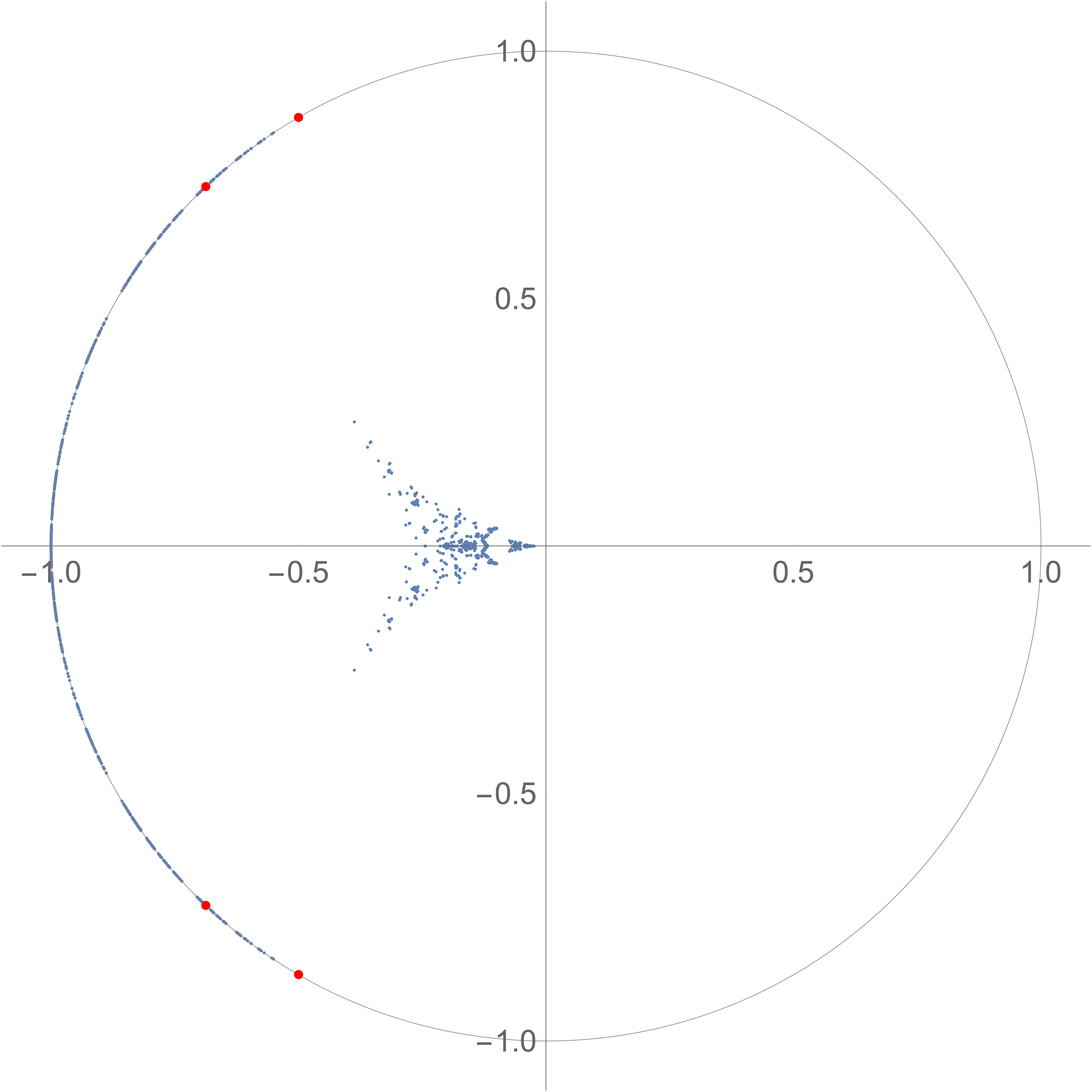 Figure 1
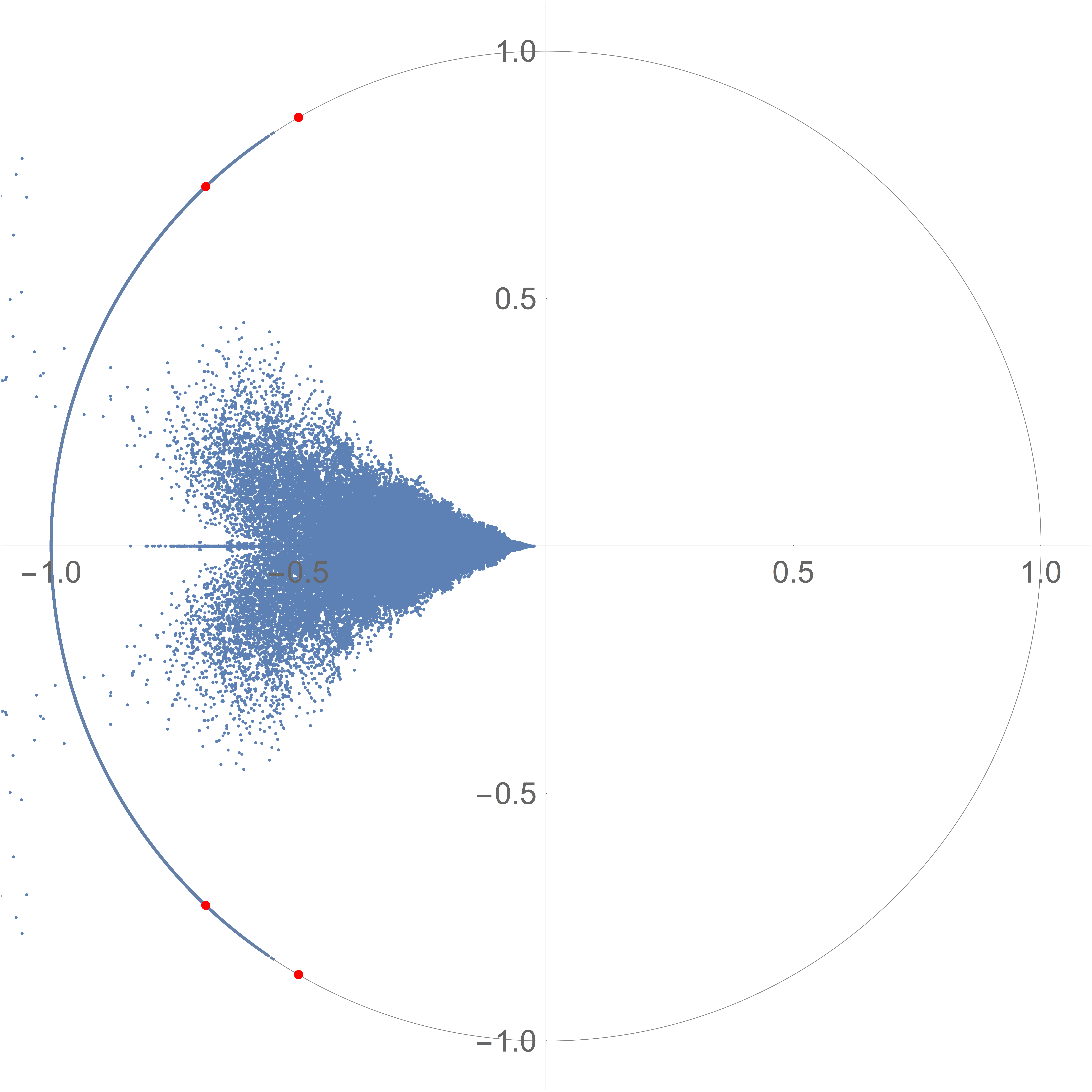 Figure 2
Peer Reviews
No public reviews on file for this paper yet. If you reviewed it on a platform where reviews are public (OpenReview, ICLR, NeurIPS, ICML), you can paste yours below so the community can read it here.
Videos
No videos yet. Explain this paper in a talk, walkthrough, or lecture? Add one.
Lee-Yang Zeros of the antiferromagnetic Ising Model
Ferenc Bencs*†*
F. Bencs: HAS Alfréd Rényi Institute of Mathematics; Department of Mathematics, Central European University; Korteweg de Vries Institute for Mathematics, University of Amsterdam
,
Pjotr Buys‡
P. Buys: Korteweg de Vries Institute for Mathematics, University of Amsterdam, Science Park 107, 1090GE Amsterdam, the Netherlands
,
Lorenzo Guerini§
L. Guerini: Korteweg de Vries Institute for Mathematics, University of Amsterdam, Science Park 107, 1090GE Amsterdam, the Netherlands
and
Han Peters
H. Peters: Korteweg de Vries Institute for Mathematics, University of Amsterdam, Science Park 107, 1090GE Amsterdam, the Netherlands
Abstract.
We investigate the location of zeros for the partition function of the anti-ferromagnetic Ising Model, focusing on the zeros lying on the unit circle. We give a precise characterization for the class of rooted Cayley trees, showing that the zeros are nowhere dense on the most interesting circular arcs. In contrast, we prove that when considering all graphs with a given degree bound, the zeros are dense in a circular sub-arc, implying that Cayley trees are in this sense not extremal. The proofs rely on describing the rational dynamical systems arising when considering ratios of partition functions on recursively defined trees.
† The research leading to these results has received funding from the European Research Council under the European Union’s Seventh Frame-work Programme (FP7/2007-2013) / ERC grant agreement n∘ 617747.
‡ Supported by NWO TOP grant 613.001.851.
§ Supported by NWO TOP grant 614.001.506.
1. Introduction
Partition functions play a central role in statistical physics. The distribution of zeros of the partition functions are instrumental in describing phase changes in a variety of contexts. More recently there has been a second motivation for studying the zeros of partition functions, arising from a computational complexity perspective. Since the 1990’s there has been significant interest in whether the values of partition functions can be approximated, up to an arbitrarily small multiplicative error, by a polynomial time algorithm. For graphs of bounded degrees this is known to be the case on open connected subsets of the zero free locus [Bar16, PR17]. In recent work of the last author with Regts [PR19, PR18], the zero free locus was successfully described by first considering a specific subclass of graphs, the Cayley trees, for which the location of zeros can be described by studying iteration properties of a rational function.
A common theme in the papers [PR19, PR18] was that the Cayley trees turned out to be extremal within the larger class of bounded degree graphs, in the sense that a maximal zero free locus for Cayley trees proved to be zero-free in the larger class as well. This observation is the main motivation for our studies here, where we investigate to which extend the extremality of the class Cayley trees holds for the antiferromagnetic Ising Model.
Let denote a simple graph and let . The partition function of the Ising model is defined as
[TABLE]
where denotes the set of edges with one endpoint in and one endpoint in . In this paper we fix and consider the partition function as a polynomial in . The case is often referred to as the ferromagnetic case, while is referred to as the anti-ferromagnetic case.
For let be the set of all graphs of maximum degree at most . Given a set of graphs , we write
[TABLE]
When , the Lee–Yang Circle Theorem [LY52a, LY52b] states that for any graph , the zeros of are contained in the unit circle . The zeros in the ferromagnetic case have subsequently been known as the Lee–Yang zeros. To study the zeros of for all one can consider the subset of finite rooted Cayley trees with down degree , which we denote by . The Lee–Yang zeros of Cayley trees are studied in [MHZ75, MH77, BM97, BG01, CHJR19] amongst other papers. In all of these papers some variation of the following rational function plays a important role:
[TABLE]
where is viewed as a function on the Riemann sphere. The significance of in relation to the Cayley trees is explained by the following lemma.
Lemma 1.1** (e.g. [CHJR19, Proposition 1.1]).**
Let and , then
[TABLE]
Thus complex dynamical systems can be used to study the zeros of the partition function of Cayley trees. The following result from [PR18] shows that while the Cayley trees from a relatively small subset of the class of all graphs of bounded maximal degree, the zero free loci of these two classes are identical in the ferromagnetic case:
Theorem 1.2**.**
Let . If then
[TABLE]
If then
[TABLE]
where is the unique parameter in the upper half plane for which has a parabolic fixed point.
Given on the unit circle, we will use notation for the closed circular arc from to , traveling counter clockwise, and similarly for open and half-open circular arcs.
When the Lee-Yang Circle Theorem fails, and the set of zeros of the partition function is considerably more complicated. Consider for example Figure 1, illustrating the location of zeros for Cayley trees and for the larger class of spherically symmetric trees, defined in Definition 1.7 below, both for maximal down-degree and maximal depth . The pictures are symmetric with respect to reflection in the unit circle, but only few zeros outside of the unit disk are depicted because of space concerns.
The pictures clearly demonstrate the appearance of zero parameters both on and off the unit circle. In this paper we focus on describing the set of zeros on the unit circle. Our main result show that, contrary to the ferromagnetic case, the zero free locus for the Cayley trees is strictly larger than that of the class of all bounded degree graphs.
We recall the following result from [PR18]:
Theorem 1.3**.**
Let be the parameter with the smallest positive angle for which . Then
[TABLE]
but
[TABLE]
Note that in Figure 1 and are depicted by the conjugate pair of red points with smallest absolute argument. The other conjugate pair of red points corresponds to and , having the same definition as in the ferromagnetic case.
Our main result is the following:
Theorem 1.4**.**
Let . If then
[TABLE]
If then
- (1)
Density for Cayley trees.**
[TABLE] 2. (2)
Nowhere density for Cayley trees.* The set*
[TABLE]
is a nowhere dense subset of . 3. (3)
Density for arbitrary graphs.* There exists such that*
[TABLE]
Case (3) will be proved in section 6, building upon results from earlier sections. Cases (1) and (2) will be proved respectively in sections 4 and 3.
Remark 1.5**.**
The fact that the closure of is strictly smaller than the closure of also holds outside of the unit circle, a statement that is considerably easier to prove. For example, the solution to the -dimensional Ising Model gives the density of zeros in a real interval , for some . On the other hand, using Corollary 3.10 one can prove the existence of a neighborhood of where all accumulation points of must lie on the unit circle.
We prove case (3) for the subclass in given by the spherically symmetric trees. These trees have the advantage that dynamical methods can be used to describe the location of zeros, as indicated by the following lemma, whose proof will be given later in this section.
Lemma 1.6**.**
Let and , then there exists a spherically symmetric tree with down degree at most for which if and only if
[TABLE]
for some .
Here is the rational semigroup generated by , i.e.
[TABLE]
We will prove that a specific sub-semigroup of is hyperbolic for all , for some , i.e. on an arc that contains . Moreover, we obtain uniform bounds on the expansion rate on compact subsets of . We also show that for any , there exists a sequence in the sub-semigroup for which lies on the Julia set. Combining these two statements we obtain uniform expansion along an orbit of . The density of zero-parameters is a consequence for sufficiently close to .
We emphasize that in statement (3) of Theorem 1.4 we only consider zero parameters in . Alternatively we can consider , which is a priori a larger set. We prove in section 6 that this closure contains the circular arc
[TABLE]
which is the arc where the earlier discussed sub-semigroup of acts hyperbolically. The parameter can be explicitly calculated. Computer evidence in fact suggests that
[TABLE]
In section 2 we prove basic results regarding the attracting intervals of the maps , to be used in later sections. In section 3 we consider the hyperbolic components in the parameter space of the maps , and prove case (2) of Theorem 1.4. In section 4 we consider only parameters on the unit circle and prove case (1).
In the remainder of this introduction we recall the relationship between partition functions on Cayley trees and spherically symmetric trees on the one hand, and respectively iteration and semi-group actions on the other hand. In particular we give a short proof of Lemmas 1.1 and 1.6. In the rest of the paper we will only consider the two dynamical systems, with few references to partition functions.
1.1 Iterates and semigroups arising from trees
Let us recall from [PR18] (but see also [CHJR19]) how the zeros of the Ising partition function on some recursively defined trees can be studied using iterations or compositions of rational functions.
Let be a marked node of a graph . Note that
[TABLE]
where sums only over with , and sums only over with . It follows that
[TABLE]
Suppose now that is a tree. Denote the neighbors of by , and the corresponding connected components of by . Then it follows that
[TABLE]
Hence when all the rooted trees are isomorphic, one obtains
[TABLE]
Definition 1.7**.**
Let and let . Let be the rooted graph with a single vertex. Recursively define the trees by letting consist of a root vertex of degree , with each edge incident to connected to the root of a copy of . We say that the rooted trees are spherically symmetric of degree at most . Equivalently a rooted tree, with root , is said to be spherically symmetric if all leaves have the same depth , and all vertices of depth have down-degree . When all degrees are equal to the tree is said to be a (rooted) Cayley tree of degree .
Note that for a spherically symmetric tree
[TABLE]
Since we will work with it follows by induction that and cannot both be equal to zero, from which it follows that
[TABLE]
Noting that , it follows for Cayley trees that
[TABLE]
where
[TABLE]
while for spherically symmetric trees we obtain
[TABLE]
Hence we have proved lemmas 1.1 and 1.6.
Motivated by this discussion we introduce the notations
[TABLE]
and
[TABLE]
where again refers to the semi-group . Thus if and only if for a Cayley tree , while if and only if for a spherically symmetric tree .
2. -stable components
Given a family of rational maps parameterized by a complex manifold , the set of -stable parameters is the set of parameters for which the Julia set moves continuously with respect to the Hausdorff topology. The concept of -stability plays a central role in the study of rational functions. We refer the interested reader to [MnSS83, McM94, Slo91] for a more detailed description of -stability.
Given a positive integer and , let be the family of rational functions given by (1) parameterized by . We will write for the set of -stable parameters and for the set of hyperbolic parameters, i.e. the values for which has no critical points nor parabolic cycles on . Recall that is a dense open set and that the set is an open and closed subset of . Whether the equality holds for the family given by (1) is a natural question, though not directly relevant for our purposes.
Given we will write for the connected component of containing the parameter .
Theorem 2.1**.**
There exists a holomorphic motion of over which respects the dynamics, i.e. there exists a continuous map satisfying
* is the identity at the base point , i.e. ,*
- 2.
for every the map is holomorphic in ,
- 3.
for every the map is injective and can be extended to a quasi-conformal map .
- 4.
for every the map is a homeomorphism. Furthermore, the following diagram commutes
[TABLE]
Such map satisfies the following two additional properties
Given the map is continuous with respect to ,
- 6.
Let be a convergent sequence and assume that is not constant. Then there exists a subsequence and so that
[TABLE]
Remark 2.2**.**
The existence of a continuous map satisfying properties was proven by [MnSS83, Slo91], while the properties and follow immediately from continuity of . The holomorphic motion is unique on the Julia set , in the sense that any other continuous map which satisfies the properties has to agree with on the set .
Define the two sets
[TABLE]
Given a connected component we further write and . Since the Julia set moves continuously for it follows that is open while is closed with respect the intrinsic topology of .
Definition 2.3**.**
Let be a connected component of . We say that is exceptional if there exists so that is constant, where denotes the holomorphic motion of over .
Remark 2.4**.**
Suppose that is an exceptional component of and let be so that the map is constant. Given another we have that , and therefore that . Let be the holomorphic motion of over . Then we have
[TABLE]
This shows that if is an exceptional component then and for every the map is constant.
Proposition 2.5**.**
Let be a connected component of . Then the set is perfect with respect to the intrinsic topology of .
Proof.
We already know that is closed in , thus we only have to show that contains no isolated points. If is an exceptional hyperbolic component, then according to Remark 2.4 we have and the result follows immediately. Assume instead that is not exceptional, let and be the holomorphic motion of over .
Since the Julia set of a rational map is perfect, it follows that we may take which converges to , and that is not identically equal to . By Theorem 2.1 we may therefore find a sequence and so that for every . Since we conclude that , proving that is not an isolated point of , and that is perfect. ∎
The definition of active parameters is classical [McM00, DF08], and was inspired by [Lev81, Lyu83]. In all these works activity is always defined in terms of the family , where is the parameterization of a critical point. For our purpose it is natural to replace with the point , even though the point is never critical.
Definition 2.6**.**
A parameter is passive if the family is normal in some neighborhood of , and is active otherwise.
We further remark that, given a marked point and the corresponding family , it would be more accurate to say that the marked point is passive/active at . However since in our case the marked point is always , we will refer to passive/active parameters instead.
Lemma 2.7**.**
Every active parameter is in .
Proof.
This is a standard normality argument. Assume first that or that . Let be an active parameter and choose so that are all distinct. Since is never a critical value of we can define two holomorphic map so that in a neighborhood of . By conjugating with a holomorphically varying family of Möbius transformation we may assume that . Since the family is not normal at , by Montel’s Theorem we conclude that it cannot avoid the three points in a neighborhood of . Since are both mapped to , the orbit cannot miss the point near , proving that . When and the point is fixed and has only two preimages . In this case we fix and we choose as one of the two preimages of , the proof is then the same as above. ∎
Lemma 2.8**.**
Let be a non-exceptional component of . Then every is passive and every is active.
Proof.
Given let be the holomorphic motion of over . If then the orbit , avoids the Julia set and in particular it avoids three distinct points . Since the set is open we have that for every sufficiently close to , and therefore the orbit of avoids the set . Using the normality argument from the proof of the previous lemma, we may therefore conclude that is normal in a neighborhood of , showing that is passive.
Suppose that there exists which is passive. Given any by equicontinuity we can find so that
[TABLE]
Given any open neighborhood there exists so that . Given with distance at least from we can therefore find so that . We conclude that we can construct a sequence converging to the point and a sequence of positive integers so that
[TABLE]
By Theorem 2.1, up to taking a subsequence of if necessary, we may assume that there exists a sequence so that and so that . This implies that
[TABLE]
By continuity of the holomorphic motion, we may further assume that whenever is sufficiently large we have
[TABLE]
In combination with the previous inequality we conclude that for every sufficiently large we have
[TABLE]
contradicting the definition of the sequence . Thus every is active. ∎
3. Dynamics of the map
For given and , we are interested in the dynamics of the map under the assumption that . In this case we have
[TABLE]
and the restriction of to is orientation reversing. If we write and for the Fatou and the Julia set of the map we conclude that
[TABLE]
When , we further have
[TABLE]
Therefore the value of increases as decreases. Recall that a rational map is expanding on an invariant set if locally increases distances, while it is uniformly expanding if distances are locally increased by a multiplicative factor, bounded below by a constant strictly greater than .
Lemma 3.1** ([PR18, Lemma 9]).**
If and then the map is uniformly expanding on . If then the map is expanding on .
Definition 3.2** ([PR18, Lemma 12]).**
Given we write for the unique parameter satisfying and for which has a parabolic fixed point.
The following proposition describes the set of hyperbolic parameters on the unit circle
Proposition 3.3**.**
We have
[TABLE]
Proof.
When then by Lemma 3.1 the map is uniformly expanding and therefore hyperbolic. When and then for every either or is uniformly bounded away from . By (4) we obtain again that the map is uniformly expanding, proving that is hyperbolic. On the other hand when the map has a parabolic fixed point, and therefore it is not hyperbolic.
Given , then are the unique parameters on the unit circle for which has a parabolic fixed point. Suppose that there exists which is not hyperbolic. By (3) the set is contained in the Fatou set, and therefore the critical points of are also contained in the Fatou set. It follows that the map must have a parabolic cycle with period at least . Since there are at most two Fatou components we conclude that the period of the parabolic cycle is exactly .
Notice that for every we have that and therefore that
[TABLE]
Let be the parabolic cycle of . These two points are parabolic fixed points for and both of them have an immediate basin that must coincide with a Fatou component of . By replacing with if necessary, we may therefore assume that is the attracting basin of , while is the attracting fixed point of . This shows that and that . And therefore that , contradicting the fact that the period of the cycle is . ∎
We notice that is always a hyperbolic parameter, therefore the set , i.e., the connected component of containing , is always well defined. On the other hand the set is defined for and does not coincide with if and only if .
Proposition 3.4**.**
Let . Then for every the Julia set is a quasi-circle, while the Fatou set contains exactly two components which are the attracting basin of a (super)attracting -cycle. If we further assume that then .
Let . Then for every the Julia set is a Cantor set, while the Fatou set coincides with the attracting component of an attracting fixed point.
Proof.
The function satisfies and . Since is a real map and maps the disk to the complement of its closure, we conclude that has a periodic point of order 2 in . By (3) it is clear that . The holomorphic motion of over given by Theorem 2.1 now implies that the Julia set is a quasi-circle for every . The two components of are mapped into each other, and by continuity the same holds for . Hyperbolicity of implies that they are the basin of a (super)attracting -cycle.
When the map has an attracting fixed point at . It is well known that the Julia set of a rational function with a single invariant attracting basin containing all the critical points is a Cantor set (see also [Mil00, Theorem B.1]). Proceeding as above we obtain that for every the set is a Cantor set and that coincides with the attracting basin of a (super)attracting fixed point. Since the critical point of are not fixed point, we conclude that the fixed point is attracting. ∎
Remark 3.5**.**
A bicritical rational map is a rational with two distinct critical points (counted without multiplicity). The space of bicritical rational map of degree was studied by Milnor [Mil00], where he shows that its Moduli space (the space of holomorphic conjugacy classes) is biholomorphic to . In this paper he constructs explicit conjugacy invariants . In our case the invariants associated to the map are given by
[TABLE]
A bicritical rational map is real if its invariants are real, or equivalently if there exists an antiholomorphic involution which commutes with the map. When , the map is real if and only if , and the corresponding involution is . The results obtained by Milnor for real maps are sufficient to conclude that given the Julia set is either a Cantor set or the whole circle.
The following definition follows from the proposition above. Recall that when by Proposition 3.3 we have and that when all fixed point of are on the unit circle.
Definition 3.6**.**
Given and , we write for the attracting fixed point of and for the connected component of containing . Notice that the map is an orientation reversing bijection .
Theorem 3.7**.**
Let . Then there exist unique parameters with , so that when
[TABLE]
Similar inclusions hold for .
The existence of and the first two inclusions follows from [PR18, Theorem 5]. Since the dynamics of is conjugate to the dynamics of it will be sufficient to prove that for .
By the implicit function theorem the point moves holomorphically in a neighborhood of , furthermore by (4) it satisfies
[TABLE]
Lemma 3.8**.**
Let . Then for every we have .
Proof.
A simple calculation shows that is an attracting fixed point for if and only if . This fact together with (5) imply that and that as . If we differentiate both sides of the equation with respect to , and then we evaluate at , we obtain
[TABLE]
Therefore for sufficiently close to the point lies in the upper half plane. However as varies within , the point moves on without intersecting . Therefore on the whole . ∎
Proof of Theorem 3.7.
Let so that . Since the map is an orientation reversing bijection, we have
[TABLE]
showing that are fixed points for . The Fatou set is connected, therefore there can be only one attracting or parabolic fixed point for , which is . This shows that the cycle is repelling. By the implicit function theorem the points move holomorphically and without collisions on some neighborhood .
By the previous lemma and (5) we have
[TABLE]
Suppose now that for some we have . By (4) the map is a contraction on . As the point moves counterclockwise on , its image moves clockwise on starting at and ending at . Since is a contraction and , this is possible only if is an orientation reversing bijection. We conclude that and thus that .
If we differentiate both sides of we obtain the equation
[TABLE]
Since it follows that is a repelling fixed point for , furthermore since we must have and . If we evaluate the expression above at we obtain that
[TABLE]
for some positive constant . If we write then we obtain that
[TABLE]
therefore as is sufficiently close to , we must have and thus that .
This also proves that the point moves counterclockwise as is close to . We will show that moves counterclockwise on the whole arc between and . Assume otherwise, then there is some such that
[TABLE]
Note that, since for any , it follows that . As a result we must have , and therefore
[TABLE]
which contradicts the fact that is a repelling fixed point of . This shows that for every and therefore , concluding the proof of the proposition. ∎
Recall that for the point is a hyperbolic parameter and that is an open and closed subset of . Therefore the connected component is a connected component of . The same is clearly true for when is a hyperbolic parameter.
Lemma 3.9**.**
For the component is not exceptional. For the component is not exceptional.
Proof.
When the component is not exceptional since is an attracting fixed point for the map .
Suppose now that is exceptional for some and let be the holomorphic motion of over . Since the holomorphic motion respects the dynamics we obtain that for every
[TABLE]
This shows that when the degree is even the function maps to a fixed point of , proving that . On the other hand, when is odd the point is periodic with period two, and therefore . Once the values of and are fixed there are only finitely many values of for which equation (7) is satisfied, giving a contradiction. ∎
Corollary 3.10**.**
Suppose that and , or alternatively that and . Then the set of accumulation points of in equals . Moreover, if the degree is even then
[TABLE]
Proof.
We first prove the statement for general degrees . By Lemmas 2.7 and 2.8 we obtain the inclusion
[TABLE]
Therefore it suffices to show that every is either an isolated point of or is not contained in . The map is hyperbolic, therefore the orbit of converges to an attracting periodic point of period . By Proposition 3.4 when the Fatou set is connected and . Similarly, when , the set is the union of two distinct connected components, and .
The parameter is passive, therefore uniformly on some small ball , where and is the holomorphic continuation of the periodic point . The point cannot be an attracting periodic point of order or , thus . We conclude that whenever is sufficiently large the point is bounded away from . Therefore the intersection only contains isolated points.
Now suppose that is even and let . Let be the first integer so that . Since is even the point is periodic with period . If the point is a repelling periodic point, since attracting fixed points in have period or . On the other hand cannot be an attracting periodic point with order or . This shows that , which proves (8). ∎
Proposition 3.11**.**
Let . Then the set is a Cantor set, with respect to the intrinsic topology of .
Proof.
Proposition 2.5 states that is a perfect set. Therefore we only need to show that every connected component of this set consists of a single point. Let be the holomorphic motion of over . By Theorem 2.1 the map is continuous and sends inside . Since is a Cantor set we conclude that is constant on , and therefore that for some and every .
If contains more then one point then by the identity principle we must have for all , and in particular , thus showing that is an exceptional component, contradicting Lemma 3.9. We conclude that is a single point. ∎
Combining the previous proposition with Corollary 3.10 we conclude the proof of claim in Theorem 1.4.
4. Restriction to the unit circle
Throughout this section it will be assumed that .
Lemma 4.1**.**
Let , and let be the holomorphic motion of over . Assume that and that one of the two following conditions is satisfied:
- (1)
the partial derivative , 2. (2)
there exist sequences both converging to and satisfying .
Then there exists a sequence converging to so that is a repelling periodic point for each map .
Proof.
Given the Julia set is contained in the unit circle. Therefore for every there exists so that the map sends inside a relatively compact subset of . By continuity of the holomorphic motion we may assume that the same is true for the map whenever is sufficiently close to . The map can be interpreted as a map between intervals. We will denote its graph as .
Assume first that condition holds. Let be a sequence of repelling periodic points so that and . Since the graph intersects the line transversally at the point . By Theorem 2.1, when is sufficiently large the graph is uniformly close to and therefore it intersects the line in for some close to . It follows that and that is a repelling point for
Assume now that condition holds. Since repelling fixed points are dense in the Julia set, we may assume from the beginning that the and are repelling fixed points for . When is sufficiently large the graphs and are both close to . Furthermore, since the map is injective, we conclude that
[TABLE]
meaning that the graph lies in between and .
It follows that when is sufficiently large there exists close to so that either or . As in the previous case we obtain that is a repelling fixed point for and that , concluding the proof of the proposition.
∎
Proposition 4.2**.**
Let be so that is a repelling periodic point for . Then .
This proposition is proved after Lemma 4.5. We claim that is enough to prove the statement for hyperbolic parameters. When by Proposition 3.3 all points in the circle are hyperbolic, and the claim is certainly true. Assume instead that and that the Proposition holds for hyperbolic parameters. Given by Corollary 3.4 the Julia set coincides with the unit circle, and by Lemma 4.1 we may find parameters in arbitrarily close to for which is a repelling periodic point. It follows that and that
[TABLE]
This shows that the proposition holds also when , proving the claim (by Proposition 3.3, non-hyperbolic point on the circle are in ).
From now on we will fix so that is a repelling point for . Given such we will write for the period of the point , and for the holomorphic motion of over .
Lemma 4.3**.**
Suppose that or that . Then there exist sequences both converging to and satisfying .
Proof.
Suppose first that or that and . In this case , and the result follows immediately.
When instead and , then by Proposition 3.4 the Julia set is a Cantor set. Suppose for the purpose of a contradiction that the Lemma were false, so that , where is a connected component of . The connected components of are open arcs which are mapped one to another by and are eventually mapped into the invariant arc containing the unique attracting fixed point .
If it follows that for some we must have . But is invariant and we are assuming that is periodic, therefore . However this is not possible when since the boundary points of are repelling periodic points with period , giving a contradiction. ∎
The point is a fixed point if and only if . If then the point is an attracting fixed point for , thus if is a repelling periodic point for we must have .
Lemma 4.4**.**
Suppose that and that . Then .
Proof.
Suppose instead that and write . Since the point is a repelling periodic point of period for it follows that
[TABLE]
For we then have , and therefore , contradicting the fact that is a repelling fixed point with period . ∎
Since is a hyperbolic parameter, there exists an integer , an open neighborhood and so that whenever are sufficiently close we have
[TABLE]
Given sufficiently small we may further assume that the same is true for when we take . Since the map is continuous with respect to the Hausdorff distance, we may further assume that for every . We therefore obtain the following:
Lemma 4.5**.**
There exists so that for every and distinct we can find so that
[TABLE]
Proof of Proposition 4.2.
Let be a parameter for which is a repelling periodic point of period . We will assume first that or that .
By Lemma 4.3 there exist two sequences in converging to ; one contained in the upper half plane and one in the lower half plane. Since the backward images of the point accumulates on the Julia set , and thus on every point in such sequences, we may find two preimages of the point contained in so that . Write for the two positive integers so that .
Take and write . Then if is sufficiently small we have and we can find two continuous functions so that and
[TABLE]
Lemma 4.3 shows that condition in Lemma 4.1 is satisfied. It follows that there exists arbitrarily close to so that is also a repelling periodic point for , and therefore . Furthermore by Lemma 3.9 the holomorphic map is not constant, therefore we may choose so that .
By Lemma 4.5 we may find so that , and since is a periodic point for of period we conclude that
[TABLE]
showing that .
The map is continuous and we have
[TABLE]
Therefore we may conclude that there exists so that either or . Since and are preimages of the point we conclude in both cases that . Since , and thus , can be chosen arbitrarily close to , we must have .
Suppose now that and that . We notice that once and are fixed, this can happen only for finitely many values of . Combining Lemma 4.4 and Lemma 4.1 we can find arbitrarily close to for which is a repelling fixed point for with period greater than . Since the proposition holds for it must hold for as well, concluding the proof of the proposition.
∎
Proof of claim in Theorem 1.4.
We already showed that Lemma 4.1 together with Proposition 4.2 imply . Therefore when by Proposition 3.3 we have
[TABLE]
If or , then is a repelling 2-cycle of , therefore by Proposition 4.2 we have . ∎
5. Hyperbolic semigroups and expanding orbits
All throughout this section we will assume that and are fixed.
Definition 5.1**.**
Given we define the semigroup as the semigroup generated by the maps
[TABLE]
We will write for the Fatou and Julia set of the map and for the Fatou and Julia set of the semigroup .
The following characterization of the semigroup will not be used later in the paper.
Proposition 5.2**.**
For all but countably many the semigroup is freely generated by .
Proof.
Let be the free group generated by and write for the homomorphism
[TABLE]
Given a word the map is a rational map in both and . Its degrees with respect to and are equal to
[TABLE]
We notice that the map is also a rational map in of degree
[TABLE]
The set is countable, therefore it is sufficient to show that for every either for finitely many or .
Suppose instead that and satisfy for infinitely many . Using the identity principle, it is not hard to show that holds for all . This shows that the maps and coincide as rational maps in both variables and , and therefore that
[TABLE]
If we now write and we obtain that also holds for infinitely many and therefore . Iterating this procedure we obtain that , concluding the proof of the proposition. ∎
Notice that for we have and hence .
Definition 5.3** (Notation).**
In order to maintain the notation readable we are avoiding (where possible) the use of the subscript . As an example, notice that we are writing instead of the more accurate . The function will play an important role in the analysis of the semigroup . Therefore we will write and for the parameters obtained by Theorem 3.7 applied to the map , and for the immediate attracting arc relative to the function (if it exists). When it is necessary to distinguish between different values of the parameter we will write and .
We will write for the set of all possible sequences with entries in . For every element we can find and so that where we write
[TABLE]
For we will further write
[TABLE]
Definition 5.4**.**
We define the length of an element as the minimum integer for which for some .
We proved in section 4 that for any in the closed arc there exists a (rooted) Cayley tree of degree and a parameter arbitrarily close to so that
[TABLE]
Recall from [PR18, Theorem B] on the other hand that for any , any and any graph of degree we have
[TABLE]
The situation for the arc appears to be more complicated. If we only consider Cayley trees of degree it is possible to show that indeed there exist zeros of the partition function of some tree on the arc . However as shown in section 3, these zeros form a nowhere dense subset of the arc. Our purpose is to show that zeros of the partition for general bounded degree graphs are dense in , where is a parameter on the unit circle close to . In order to do so we will consider the class of rooted spherically symmetric trees of bounded degree for which, according to Lemma 1.6, the zero parameters can be understood by studying the semigroup dynamics of .
In what follows we will study the semigroup dynamics (mostly) under the assumption that . Under these assumptions for any we have , and therefore that
[TABLE]
5.1 Hyperbolicity of the semigroup
Lemma 5.5**.**
There exists so that for every and every we have
[TABLE]
Proof.
Assume first that and recall that by Theorem 3.7 we have . The Möbius transformation is a bijection of the unit circle into itself which revers the orientation, and . The map is an orientation reversing bijection and therefore satisfies . It follows immediately that, if we write for the length of the arc , the image is an arc of length , therefore the map is not surjective.
Notice that when the point move counterclockwise on the arc starting at the point , its image moves clockwise on the unit circle, starting at , until it reaches . In principle it is possible that rotates once or more times around the circle, however since is not surjective on this does not happen. We conclude that is also an orientation reversing bijection, and since the length of the arc is less than the length of , we must have . If we now compose with the map we find that
[TABLE]
Since moves continuously in , the same holds sufficiently close , which implies the existence of . ∎
In the following we will denote by the parameter with the maximal argument that satisfies the requirements of the previous lemma.
Definition 5.6**.**
We define the semigroup as the semigroup generated by the maps
[TABLE]
where and for . We will write for the Fatou and the Julia set of the semigroup .
Since , it follows that . Furthermore by the previous lemma the interval is invariant for every map in for , and therefore it is contained in , proving that for these
[TABLE]
and therefore that the Fatou set is connected.
Similarly to the case of the semigroup , given and we will write
[TABLE]
Also in this case every element of the semigroup can be written as for some and .
By the previous lemma, given it follows that there exists a closed arc so that for every . Indeed, if we write , this property is satisfied by , where is sufficiently close to and lies in (where the preimage is taken inside ). We may therefore define the family and the closed arc as follows:
[TABLE]
In this definition refers to the interior of with respect to the topology of the unit circle.
Lemma 5.7**.**
Let . Then the set is a non-empty closed arc which is forward invariant under . Furthermore the map is upper semi-continuous for .
Proof.
Write for the subset of all intervals whose extrema are rational angles. Notice that given there exists for which , and therefore
[TABLE]
Given we have that and , proving that the arc contains the unique attracting fixed point of . This shows that for any pair the intersection is non empty. Furthermore one can show that is again an element of . Similarly given one has that .
The set is countable, hence we can enumerate its elements as . If we write it then follows that , that and that
[TABLE]
This shows that is the intersection of a nested family of non-empty, compact and connected arcs, and therefore that is a non-empty closed arc. Since every is forward invariant for any , the same holds for .
We will now write in order to study parameter values close to . On the other hand we will write for the set defined above for the parameter value . For every positive integer we have for every sufficiently close to , and for such parameters it then follows that . Since is a sequence of nested sets approximating we conclude immediately that the map is upper-semicontinuous at the point , concluding the proof of the lemma. ∎
Proposition 5.8**.**
Let . Then every limit of a convergent sequence in with divergent length is constant on and contained in .
Proof.
Let be a sequence with divergent length that converges uniformly to . Choose sequences and so that , and notice that since the sequence has divergent length we must have . Since , it follows that is connected. Write for the hyperbolic metric of .
The Fatou set is forward invariant with respect to each element in the semigroup. In particular we have . Since the closed arc is forward invariant, it contains the unique attracting fixed point of (which coincides with the attracting fixed point of ). Assume now that . Since is invertible, it then follows that the Fatou set is completely invariant with respect to , and therefore it contains the whole attracting basin of . Since is a Möbius transformation, we conclude that the Julia set of the semigroup must consist of a single point, giving a contradiction. Therefore
[TABLE]
For every the map has two critical points . It follows from the Schwarz-Pick Lemma that for every the map is a contraction with respect to the metric . This means that for every compact set we may find a constant so that for any we have
[TABLE]
Let as in (11), and define , where the ball is taken with respect to the hyperbolic metric of . Given and , we know that for every we have and
[TABLE]
This shows that , and thus that
[TABLE]
which finally implies that for every . We took to be arbitrary and thus we can conclude that is constant. For every and it follows that , completing the proof. ∎
We recall the following definition of hyperbolicity for semigroups, introduced in [Sum97, Sum98].
Definition 5.9**.**
Let be a rational semigroup and consider the postcritical set
[TABLE]
We say that the semigroup in hyperbolic if .
Proposition 5.10**.**
The semigroup is hyperbolic.
Proof.
In our case the postcritical set can be written as
[TABLE]
It is clear that for every and . Furthermore, by the previous theorem we know that every limit point belongs to , showing that
[TABLE]
∎
Given we write for the Fatou and Julia sets of the family . By (10) we have that
[TABLE]
and one can show that if its orbit avoids the set . On the other hand given , by Proposition 5.8 we can find so that . We conclude that we can write
[TABLE]
The following lemma shows expansivity of the dynamics on the Julia set of every sequence . The result corresponds to [Sum98, Theorem 2.6]; for the sake of completeness we provide a sketch the proof.
Lemma 5.11**.**
Let and . Then there exists a positive integer so that for any and we have
[TABLE]
Sketch of the proof..
We start by choosing an open simply connected neighborhood containing and two open simply connected neighborhoods containing and disjoint from and . Then choose so that , where we write for the infinitesimal hyperbolic metric of the two sets.
By Proposition 5.8 there exists a positive integer so that
[TABLE]
Given and , by (12), we have for every . Therefore we may define as the connected component of containing . Since is simply connected and disjoint from the postcritical set, the map preserves the hyperbolic metrics of and . Since , this implies that
[TABLE]
The hyperbolic metric of and the Euclidean metric are comparable on . Therefore by taking an integer sufficiently large, which does not depend on the choice of the sequence and , we conclude that the value satisfies the requirements of the Lemma.
∎
We will now show that, once we are bounded away from , the value of can be chosen independently from . It will be convenient to reintroduce the subscript in order to distinguish between different parameter values. It is clear the set is dependent on , thus it will be denoted as .
Lemma 5.12**.**
Let and . Then there exists a positive integer so that for any , any and any there exists so that
[TABLE]
Proof.
Given let be the minimum integer for which the previous lemma is valid. Suppose now that there exists a sequence such that . It follows that we may find sequences and , so that
[TABLE]
By passing to a subsequence if necessary, we may assume that the three following conditions are satisfied
- (1)
the parameters converge to ; 2. (2)
the points converge to ; 3. (3)
the sequences and agree on the first elements.
Since the arc varies continuously in and by (12) every it follows that . Let be the sequence given by , where denotes the -th element of the sequence . Then it is clear that and agree on the first elements. Given we have
[TABLE]
proving that . Furthermore, when is sufficiently large we have , therefore
[TABLE]
contradicting the previous lemma. ∎
Proposition 5.13**.**
Let and . Then there exists a positive integer so that for any , any and any we have
[TABLE]
Proof.
Let as in the previous lemma. For any , any and any the rational map has no critical points on the unit circle. We may therefore find a constant such that
[TABLE]
Let so that .
Suppose now that , that and that . Thanks to the previous lemma there exist positive integers and which satisfy and so that the following holds: if we write and then for
[TABLE]
showing that
[TABLE]
By choosing instead of , we conclude the proof of the proposition. ∎
5.2 Existence of expanding sequences
Lemma 5.14**.**
Given , , and there exists a such that
[TABLE]
is an element of the interval when reduced modulo .
Proof.
Note that either or , since . We consider these two cases separately.
If then for all . It follows that for any open interval contained in the interval , there exists an integer such that . Since and , there exists a such that .
Now assume that and define
[TABLE]
Observe that , and thus . Therefore it suffices to find a for which . Such a can be found by the same argument as above, because , and . ∎
Proposition 5.15**.**
Let and . Then for every there exists so that .
Proof.
Choose so that . The function can be written as , where is a Möbius transformation that fixes the unit circle. It follows that we can find disjoint sets such that
[TABLE]
ordered in such a way that for all we have
[TABLE]
Since inverts the orientation of the unit circle and , we have for close enough to that . Furthermore by Theorem 3.7 we cannot have . This shows that one of the connected component of is of the form . This component must contain the arc . Since , we find that .
Now let denote the inverse arcs of under the map in such a way that for all . Then we see that . We now present a way to choose, given a , an integer such that .
- •
If , we can choose because then .
- •
If but , we see that for some and thus we can write
[TABLE]
for some . We find that
[TABLE]
According to Lemma 5.14, we can choose in such a way that . Since , we conclude that .
This procedure defines the first steps of the sequence and satisfies for all . By iterating this procedure for the point we find a sequence such that for all . By (12) we conclude that . ∎
Let and . Then we can modify the procedure described in the proof above to obtain the following:
Proposition 5.16**.**
Let and . Then for every there exists so that and
[TABLE]
Corollary 5.17**.**
For every we have
[TABLE]
Proof.
Given choose so that , which exists according to Proposition 5.15. For every positive integer by Proposition 5.13 we may find some such that
[TABLE]
showing that and therefore that . The two equalities follow from (10). ∎
6. Zeros for the semigroup
Our goal in this section is to give a more precise description of the zeros of in for trees that are spherically symmetric of bounded degree. We will prove case (3) of Theorem 1.4:
Theorem 6.1**.**
Let . Then there exists so that the set of zero parameters for spherically symmetric trees of degree contains a dense subset of .
We will also prove the following weaker statement, which we will however prove for a considerably larger circular arc.
Theorem 6.2**.**
Let . Then the closure of the set of zero parameters of spherically symmetric trees of degree contains .
6.1 Proof of Theorem 6.1
Since we will repeatedly deal with distinct values of the parameter , we will always use the subscript in order to specify the map that we are using.
Choose a parameter value . By Proposition 5.13 there exists a positive integer so that for every , any and any we have
[TABLE]
Having fixed , it follows from the compactness of that there exists a constant so that for any and any we have
[TABLE]
Lemma 6.3**.**
There exist and a positive integer so that for every and we have
[TABLE]
Proof.
The point is a repelling periodic point of order for the map , meaning that . Writing we obtain
[TABLE]
Observing that it follows that when for sufficiently large:
[TABLE]
By continuity there exists so that
[TABLE]
Given we write for the two boundary points of . These boundary points form a repelling -cycle, hence by the implicit function theorem they vary holomorphically in an open neighborhood of . By exchanging the order of and if necessary, we may assume that . By Theorem 3.7 for every we have .
The point clearly belongs to . Recall that the map preserves the orientation of the unit circle. Since is a repelling fixed point, by replacing with a parameter in sufficiently close to so that the point remains close to for every , we may assume that . Up to replacing at each step with a parameter closer to , we may therefore assume that also , concluding the proof of the lemma. ∎
By Proposition 4.2 we know that zero parameters accumulate on . From now until the end of the proof of Theorem 6.1 we will fix the value of the parameter .
By Theorem 3.7 we know that . This fact together with (14) and (13) implies the existence of the following constant:
Definition 6.4** (Choice of the constant ).**
There exists a sufficiently small constant so that the following three conditions are satisfied:
- a.
The distance between the attracting interval and is at least ,
[TABLE]
- b.
For any we have
[TABLE]
- c.
For any , any and any we have
[TABLE]
Definition 6.5** (Choice of the sequence ).**
we define a sequence of the form
[TABLE]
where is chosen such that for all . The existence of such sequence is guaranteed by Proposition 5.16, and we have .
Lemma 6.6**.**
For every there exists a positive integer so that
[TABLE]
Proof.
Suppose on the other hand that there exists so that for every .
Since , it follows in particular . Therefore after the first steps we obtain that
[TABLE]
Write for the left shift map, and define and . Thanks to the choice of the sequence it follows that and that
[TABLE]
We claim that for every we have , where and . The claim certainly holds for . We will now assume it holds for and prove that it holds for .
By the assumption on we know that for every . Therefore, thanks to the choice of the constants and , we conclude that
[TABLE]
It then follows that for every we must have , which is possible only if , giving a contradiction. ∎
Lemma 6.7**.**
There exists a positive integer so that every point in lies at distance at most from the set
[TABLE]
Proof.
By Corollary 5.17 we have . The semigroup has no exceptional points, therefore the collection of all preimages of a given point in accumulates on the whole Julia set, and therefore on .
Writing we therefore conclude that
[TABLE]
By compactness of we may find so that still covers the set . Every is the preimage of some element of length , meaning that there exists so that
[TABLE]
By taking we obtain
[TABLE]
concluding the proof of the lemma. ∎
Write . For every there exists and so that
[TABLE]
No element in the semigroup can have critical points on the unit circle. Therefore by the implicit function Theorem there exists a holomorphic map defined in a neighborhood of so that
[TABLE]
By taking sufficiently small we may assume that for every the map is defined on and that
[TABLE]
Given we choose in such a way that . We note that this last condition is not necessary, but simplifies the proof.
By Lemma 6.6 we may choose so that . Given , write .
Proposition 6.8**.**
There exists and so that
Proof.
By the definition of we have that and by the choice of the constant we know that . Therefore, by replacing with another parameter closer to in such a way that the value of does not change, we may further assume that for every .
The image of the map contains either or (notice that one of the two possibility occurs, since the image does not intersect ). We will prove the proposition assuming that the first case occurs, a similar proof works in the other case.
Choose a point so that the distance of the point from both the extrema of the arc is bigger or equal to , which is possible since . Let so that . It then follows that and that
[TABLE]
and thanks to the fact that we conclude that
[TABLE]
and therefore that there exists so that . ∎
Let and as in the previous lemma, and let and so that . We conclude that
[TABLE]
concluding the proof of Theorem 6.1.
6.2 Proof of Theorem 6.2
Let . By Proposition 5.13 there exists a positive integer so that for any any and any we have
[TABLE]
Once is fixed we have the following:
Lemma 6.9**.**
There exist constants so that for any , any , and any , there exists a holomorphic map with , satisfying:
- (1)
[TABLE] 2. (2)
given any and any there exists a positive integer so that
[TABLE]
Proof.
Note that the second derivative of is bounded in a neighborhood of . It follows that for and sufficiently small, the maps are uniformly expanding in a given neighborhood of . The existence of the point follows immediately. The fact that can be given as the limit of a sequence of contracting inverse branches implies the holomorphic dependency on . ∎
Proposition 6.10**.**
Let . Then the family of maps
[TABLE]
is not normal near .
Proof.
Let as in the previous lemma. By Lemma 5.7 the map is upper semi-continuous in , and is continuous. Therefore by compactness of , and by taking smaller if necessary, we may assume that
[TABLE]
Now assume for the purpose of a contradiction that the family of holomorphic functions is normal near . By Ascoli–Arzelá Theorem it follows that there exists so that for every we have
[TABLE]
By Proposition 5.16 we can fix so that and for every positive integer . It follows that , on the ball . By the identity principle it follows that on the bigger ball , where is the map defined in the previous lemma.
Now notice that given we have . If this were not the case then by (10) we could find a positive integer so that , and by Proposition 5.8 we conclude that . In particular when is sufficiently large the point lies at distance strictly less than from the set . Since instead the point lies in and the two sets and have distance greater than , we conclude that for sufficiently large
[TABLE]
contradicting the fact that .
On the intersection the maps and are well defined. For every and every positive integer we have and
[TABLE]
which implies that
[TABLE]
and thus that on the open set . By the identity principle it follows that on . By iterating this procedure we conclude that for every we have and on the all ball . It follows that .
Recall that by Theorem 3.7 we have , therefore by Lemma 5.5 we have if and only if . Hence for every we must have
[TABLE]
which implies that for all , which contradicts Lemma 3.9. This concludes the proof of the proposition. ∎
Theorem 6.2 now follows from Montel’s Theorem as in Lemma 2.7.
The reference list from the paper itself. Each links out to its DOI / PubMed record.
- 1[Bar 16] A. Barvinok, Combinatorics and complexity of partition functions , Algorithms and Combinatorics, vol. 30, Springer, Cham., 2016.
- 2[BG 01] J. C. A. Barata and P. S. Goldbaum, On the distribution and gap structure of Lee–Yang zeros for the Ising model: Periodic and aperiodic couplings , Journal of Statistical Physics 103 (2001), no. 5/6, 857–891.
- 3[BM 97] J. C. A. Barata and D. H. U. Marchetti, Griffiths' singularities in diluted Ising models on the Cayley tree , Journal of Statistical Physics 88 (1997), no. 1-2, 231–268.
- 4[CHJR 19] I. Chio, C. He, A. L. Ji, and R. K. W. Roeder, Limiting measure of Lee–Yang zeros for the Cayley tree , Communications in Mathematical Physics (2019).
- 5[DF 08] R. Dujardin and C. Favre, Distribution of rational maps with a preperiodic critical point , Amer. J. Math. 130 (2008), no. 4, 979–1032.
- 6[Lev 81] G. M. Levin, Irregular values of the parameter of a family of polynomial mappings , Uspekhi Mat. Nauk 36 (1981), no. 6(222), 219–220.
- 7[LY 52a] T. D. Lee and C. N. Yang, Statistical theory of equations of state and phase transitions. I. Theory of condensation , Physical Rev. (2) 87 (1952), 404–409. MR 0053028
- 8[LY 52b] by same author, Statistical theory of equations of state and phase transitions. II. Lattice gas and Ising model , Physical Rev. (2) 87 (1952), 410–419. MR 0053029