Global Stabilization of 2D Forced Viscous Burgers' Equation Around Nonconstant Steady State Solution by Nonlinear Neumann Boundary Feedback Control:Theory and Finite Element Analysis
Sudeep Kundu, Amiya Kumar Pani

TL;DR
This paper develops a nonlinear boundary feedback control method to achieve global stabilization of the 2D forced viscous Burgers' equation around a nonconstant steady state, with finite element analysis and numerical validation.
Contribution
It introduces a novel nonlinear Neumann boundary feedback control for stabilizing the 2D Burgers' equation around nonconstant steady states, including error estimates and convergence analysis.
Findings
Global stabilization achieved under smallness condition.
Optimal error estimates in $L^ abla(L^2)$ and $L^ abla(H^1)$ norms.
Numerical experiments confirm theoretical results.
Abstract
Global stabilization of viscous Burgers' equation around constant steady state solution has been discussed in the literature. The main objective of this paper is to show global stabilization results for the 2D forced viscous Burgers' equation around a nonconstant steady state solution using nonlinear Neumann boundary feedback control law, under some smallness condition on that steady state solution. On discretizing in space using piecewise linear elements keeping time variable continuous, a semidiscrete scheme is obtained. Moreover, global stabilization results for the semidiscrete solution and optimal error estimates for the state variable in and -norms are derived. Further, optimal convergence result is established for the boundary feedback control law. All our results in this paper preserve exponential stabilization property. Finally, some…
Click any figure to enlarge with its caption.
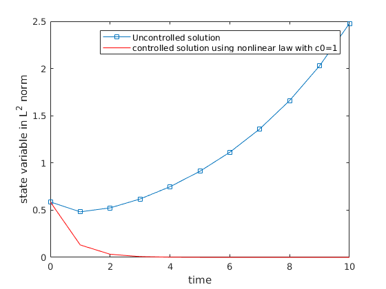 Figure 1
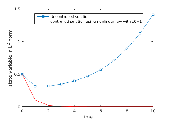 Figure 2
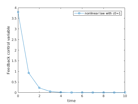 Figure 3
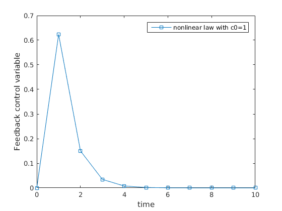 Figure 4
| Conv. Rate | Conv. Rate | |||
|---|---|---|---|---|
| 1.8401 | 0.9844 | |||
| 1.934 | 1.019 | |||
| 1.9135 | 1.047 |
| Conv. Rate | ||
|---|---|---|
| 1.7211 | ||
| 1.8409 | ||
| 1.8595 |
Peer Reviews
No public reviews on file for this paper yet. If you reviewed it on a platform where reviews are public (OpenReview, ICLR, NeurIPS, ICML), you can paste yours below so the community can read it here.
Videos
No videos yet. Explain this paper in a talk, walkthrough, or lecture? Add one.
Taxonomy
TopicsStability and Controllability of Differential Equations · Advanced Mathematical Modeling in Engineering · Advanced Mathematical Physics Problems
Global Stabilization of 2D Forced Viscous Burgers’ Equation Around Nonconstant Steady State Solution by Nonlinear Neumann Boundary Feedback Control:Theory and Finite Element Analysis
Sudeep Kundu111 Institute of Mathematics and Scientific Computing, University of Graz, Heinrichstr. 36, A-8010 Graz, Austria, Email:[email protected] and Amiya Kumar Pani222 Department of Mathematics, IIT Bombay, Powai, Mumbai-400076, India, Email:[email protected]
Abstract
Global stabilization of viscous Burgers’ equation around constant steady state solution has been discussed in the literature. The main objective of this paper is to show global stabilization results for the 2D forced viscous Burgers’ equation around a nonconstant steady state solution using nonlinear Neumann boundary feedback control law, under some smallness condition on that steady state solution. On discretizing in space using piecewise linear elements keeping time variable continuous, a semidiscrete scheme is obtained. Moreover, global stabilization results for the semidiscrete solution and optimal error estimates for the state variable in and -norms are derived. Further, optimal convergence result is established for the boundary feedback control law. All our results in this paper preserve exponential stabilization property. Finally, some numerical experiments are documented to confirm our theoretical findings.
Keywords: Forced viscous Burgers’ equation, boundary feedback control, stabilization, finite element method, error estimate, numerical experiments
AMS subject classification: 35B37, 65M60, 65M15, 93B52, 93D15
1 Introduction
Consider the following two-dimensional forced viscous Burgers’ equation with Neumann boundary control : seek which satisfies
[TABLE]
where is a bounded subset in with smooth boundary, is a constant, is a scalar control input, , is the diffusive term, is the nonlinear convective term, forcing function is independent of the time and is a given function. When , it is called inviscid Burgers’ equation, which is studied in nonlinear wave propagation.
For one dimensional Burgers’ equation, local stabilization results are documented in [5], [6] for distributed and Dirichlet boundary control and in [7] for Neumann boundary control with small initial data. For more details, see [11], [12] and [18]. Using linear feedback control law for the linearized part as in Navier-Stokes equations [20], local stabilizability results can be proved for the two dimensional Burgers’ equation. In [23], the authors have shown local stabilization results for the two dimensional Burgers’ equation directly through a nonlinear feedback control law and several numerical experiments are also reported in their article conforming their theoretical results. Subsequently Buchot et al. [4] have derived local stabilization results in the case of partial information for the two dimensional Burgers’ type equation.
Based on Lyapunov type functional, global stabilization result around constant steady state solution for one dimensional Burgers’ equation is derived in [13] and [3] for both Dirichlet and Neumann boundary control laws. For more detailed references, we refer to [17], [21] and [22]. In [8], authors implement Dirichlet boundary feedback control law on the obstacles for two dimensional Burgers’ equation by solving both Riccati equation and Chandrasekhar equations. In [14], it is shown that using a nonlinear Neumann boundary feedback control laws, solution of 1D Burgers’ equation converges exponentially to its constant steady state solution in , , and norms. Then, an application of finite element method in spatial direction yields a semidiscrete system and global stabilization results are proved for the semidiscrete approximation. Finally, optimal error estimates for the state variable and superconvergence result for the control laws are established. This analysis is then extended to 2D Burgers’ equation in [15], and stabilization results depicting convergence of the solution to its constant steady state solution are derived. Moreover, convergence result for the nonlinear feedback control law is also documented.
But when the steady state solution is non constant in the case of forced viscous Burgers’ equation, it is not known whether global stabilization results still holds or not. Also, when applying finite element method, no result is available in the literature on rate of convergence. Hence, in this paper, an attempt has been made to fill this gap.
Now the corresponding equilibrium or steady state problem becomes: find as a solution of
[TABLE]
To achieve
[TABLE]
it is enough to consider where and satisfies
[TABLE]
The motivation to choose Neumann boundary control comes from the physical situation. For instance, in thermal problem, one can not actuate the temperature , but the heat flux . Here, the control variable is to be chosen as a function of appropriately. In this article, we first prove global stabilization results in , - norms for the problem (1.6)-(1.8) with control law (3.1). Then, - conforming finite element method is applied to discretize the spatial variable, keeping time variable continuous and global stabilization results are proved for the semidiscrete solution. Further, optimal error estimates are derived for the state variable and superconvergence results are obtained for the nonlinear Neumann boundary feedback control law.
The rest of the paper is organized as follows. Section contains notations, preliminary results and properties of the steady state solution. In Section we focus on global stabilization results using nonlinear feedback control law. Section deals with finite element approximation and global stabilization results for the semidiscrete system. Further, optimal error estimates are obtained for the state variable and convergence result is derived for the feedback control law. Finally, Section concludes with some numerical experiments.
2 Notations and properties of steady state solution
In this section, we discuss some properties for the steady state problem (1.4)-(1.5) along with some preliminary results.
Throughout this paper, we use standard Sobolev space with norm and seminorm . For it corresponds to the usual norm and is denoted by . Moreover, and denote the innerproducts in and respectively. Also we use the Sobolev space of order . The space consists of all strongly measurable functions with norm
[TABLE]
and
[TABLE]
When there is no confusion we denote by . For a trilinear form \Big{(}v\big{(}\nabla w\cdot{\bf{1}}\big{)},\phi\Big{)}, denote by B\big{(}v;w,\phi\big{)}:=\Big{(}v\big{(}\nabla w\cdot{\bf{1}}\big{)},\phi\Big{)}.
Now we present a few well known theorems and inequalities which are crucial for our analysis.
Theorem 2.1**.**
([25]) (Brouwer’s fixed point theorem): Let be a finite dimensional Hilbert space with inner product and norm Let be a continuous function. If there is a real number such that with then there exists such that and
The following trace embedding result holds for 2D.
**Boundary Trace Embedding Theorem (page [1]): ** There exists a bounded linear map
[TABLE]
such that
[TABLE]
for each . Below, we recall the following inequalities for our subsequent use
Friedrichs’s inequality: (See [15]) For there holds
[TABLE]
where is Friedrichs’s constant. More explicitly
[TABLE]
Hence the Friedrichs’s constant can be taken as .
Gagliardo-Nireberg inequality (see [19]): For
[TABLE]
Agmon’s inequality (see [2]): For there holds
[TABLE]
2.1 Some properties of the steady state problem
Let be the quotient space. Infact, is a norm on this space. We now make the following assumption:
Assumption
[TABLE]
where and with N_{1}=\sup_{v,\hskip 2.84544ptz,\hskip 2.84544pt\phi\in H^{1}/\mathbb{R}}\frac{B\big{(}v;z,\phi\big{)}}{\left\lVert\nabla v\right\rVert\left\lVert\nabla z\right\rVert\left\lVert\nabla\phi\right\rVert} and N_{2}=\sup_{v\in H^{1}/\mathbb{R},\hskip 2.84544pt(z,\phi)\in(H^{1}(\Omega))^{2}}\frac{B\big{(}v;z,\phi\big{)}}{\left\lVert\nabla v\right\rVert\left|\!\left|\!\left|z\right|\!\right|\!\right|\left|\!\left|\!\left|\phi\right|\!\right|\!\right|}.
The assumption provides bound for the steady state problem (1.4)-(1.5).
Lemma 2.1**.**
Under the assumption , there exists a solution of (1.4)-(1.5) satisfying the following estimate:
[TABLE]
In addition, if and , then .
Proof.
Multiply (1.4) by to obtain
[TABLE]
Therefore
[TABLE]
Using assumption , it follows that
[TABLE]
that is,
[TABLE]
Hence, when both the factor is negative, we obtain and .
Multiply (1.4) by to arrive using the bounds of and at
[TABLE]
where the constant is appeared in the Gagliardo Nirenberg inequality.
Hence when , \left\lVert\Delta u^{\infty}\right\rVert\leq C\Big{(}\nu,\left\lVert f^{\infty}\right\rVert\Big{)}.
Now below, we provide the proof for the existence of a weak solution which satisfy (2.3). Corresponding weak formulation for the steady state solution (1.4)-(1.5) is to seek such that
[TABLE]
Let be an orthogonal basis for . Denote and finite linear combination of are dense in . We look for such that
[TABLE]
It is sufficient to verify (2.6) for , . Let . For such , we relate a unique element by . This establishes a linear bijection between and . Since are orthogonal in , . Now we define by
[TABLE]
Hence (2.6) has a solution if there exists a such that . It is valid that
[TABLE]
Using the bound for the steady state solution , we get
[TABLE]
Hence if is chosen large enough such that , we have
[TABLE]
From the condition , infact we can take . Further by (2.6), and is independent of . Since is uniformly bounded in , so there exists a convergent subsequence still denoted by such that in . Since is compactly embedded in , then there exists a convergent subsequence still denoted by such that in .
Hence by Brouwer’s fixed point theorem 2.1, there exists a such that and .
Let . From (2.6), we obtain
[TABLE]
Clearly
[TABLE]
For the nonlinear term, we can rewrite
[TABLE]
Boundedness of and , strong convergence of in norm and compact embedding of onto with implies that right hand side goes to zero in the above inequality. Hence when goes to infinity, we obtain
[TABLE]
By density, (2.7) is true for all . ∎
3 Stabilization results
Before proceeding, let us first construct the feedback control law . To obtain , we consider Lyapunov energy functional . Then
[TABLE]
Using the notation B\big{(}\cdot;\cdot,\cdot\big{)} for trilinear term, we can bound the right hand term as
[TABLE]
and
[TABLE]
Hence, we get
[TABLE]
Now, choose the Neumann boundary feedback control law as
[TABLE]
to obtain
[TABLE]
C_{LYP}=\frac{2}{C_{F}}\min\Big{\{}\frac{7\nu}{8},\frac{c_{0}}{2}+\frac{7\nu}{8}\Big{\}}. Now, satisfies the weak formulation of (1.6)-(1.8) as
[TABLE]
with where . Throughout the paper is a generic positive constant independent of the discretizing parameter .
Further we make the following assumption
Assumption
- •
Let , .
- •
Compatibility conditions at \Big{(}\frac{\partial w_{0}}{\partial n}=v_{2}(x,0),\frac{\partial w_{t}}{\partial n}(x,0)=v_{2t}(x,0)\Big{)} are satisfied.
- •
There exists a unique weak solution of (3.2) satisfying the following regularity result
[TABLE]
Our main objective in this section is to establish global stabilization results for the state variable of the continuous problem (3.2). Throughout the paper, all the results hold under the assumptions and with the same decay rate
[TABLE]
Lemma 3.1**.**
Assume that assumption is satisfied and is a steady state solution satisfying (2.3) of (1.4)-(1.5). Let . Then, there holds
[TABLE]
where \delta=\min\{\Big{(}\frac{7\nu}{4}-2\alpha C_{F}\Big{)},\Big{(}c_{0}+\frac{7\nu}{4}-2\alpha C_{F}\Big{)}\}>0, and is the constant in the Friedrichs’s inequality (2.2).
Proof.
Set in (3.2) to obtain
[TABLE]
For the first term on the right hand side of (3.4), we use integration by parts for the first sub-term and then bound it as follows
[TABLE]
Similarly, using the Young’s inequality, the second term on the right hand side of (3.4) is bounded by
[TABLE]
Now, using the Friedrichs’s inequality (2.2), it follows that
[TABLE]
Hence, from (3.4), we arrive using (3.5), (3.6) and (3.7) at
[TABLE]
Choose as (3.3), so that the coefficients on the left hand side of (3) are non-negative. Integrate (3) from [math] to and then, multiply the resulting inequality by to obtain
[TABLE]
This completes the proof. ∎
Remark 3.1**.**
The above Lemma also holds for that is,
[TABLE]
*Moreover, using the Friedrichs’s inequality, it follows that *
[TABLE]
Remark 3.2**.**
If we define the before mentioned Neumann control on some part of the boundary denoted by where measure of is non zero with remaining part zero Dirichlet boundary condition, still the stabilization result holds. For instance, consider with , where and are sufficiently smooth. Hence, from (3.4), we arrive at
[TABLE]
Using the Friedrichs’s inequality \left\lVert v\right\rVert^{2}\leq C_{F}\Big{(}\left\lVert\nabla v\right\rVert^{2}+\left\lVert v\right\rVert^{2}_{L^{2}(\Gamma_{N})}\Big{)}, it follows that
[TABLE]
This complete the rest of the proof for - stabilization. Stabilization result also holds similarly in higher order norms when control works on some part of the boundary.
Lemma 3.2**.**
Assume that assumption is satisfied and is a steady state solution satisfying (2.3) of (1.4)-(1.5). Let Then, there holds
[TABLE]
Proof.
Form an - inner product between (1.6) and to obtain
[TABLE]
The fourth term on the left hand side of (3.11) can be rewritten as
[TABLE]
The terms on the right hand side of (3.11) are bounded by
[TABLE]
and using Lemma 3.1
[TABLE]
Finally, using the bounds of , we arrive from (3.11) at
[TABLE]
Integrate the above inequality from [math] to and then use the Grönwall’s inequality with Lemma 3.1 to obtain
[TABLE]
Use Remark 3.1 for the integral term under the exponential sign, and then multiply the resulting inequality by to complete the rest of the proof. ∎
Lemma 3.3**.**
Assume that assumption is satisfied and is a steady state solution satisfying (2.3) of (1.4)-(1.5). Let . Then, the following estimate holds
[TABLE]
Proof.
Choose in (3.2) to obtain
[TABLE]
The terms on the right hand side of (3.13) are bounded by
[TABLE]
and using Lemma 3.1
[TABLE]
Hence, rewriting the boundary integral term in (3.13) as in previous Lemma 3.2, we arrive from (3.13) at
[TABLE]
Apply Lemmas 3.1 and 3.2, and the Grönwall’s inequality to the above inequality to complete the rest of the proof. ∎
Lemma 3.4**.**
Assume that assumptions and are satisfied and is a steady state solution satisfying (2.3) of (1.4)-(1.5). Then, there holds
[TABLE]
Proof.
Differentiate (1.6) with respect to and then take the inner product with to obtain
[TABLE]
The first right hand side term in (3.14) is bounded by
[TABLE]
The other right hand term in (3.14) is bounded by
[TABLE]
Therefore, from (3.14), we obtain
[TABLE]
To calculate take the inner product between (1.6) and to obtain at
[TABLE]
Integrate the inequality (3.15) from [math] to and then use Lemmas 3.1-3.3 to complete the rest of the proof. ∎
Lemma 3.5**.**
Assume that assumptions and are satisfied and is a steady state solution satisfying (2.3) of (1.4)-(1.5). Then the following estimate holds
[TABLE]
Proof.
Differentiate (1.6) with respect to and then take inner product with to obtain
[TABLE]
The first three terms on the right hand side of (3.16) are bounded by
[TABLE]
and using Lemma 3.1
[TABLE]
The boundary term on the right hand side of (3.16) is bounded by
[TABLE]
Hence, from (3.16), we arrive at
[TABLE]
Integrate the above inequality from [math] to and then apply the Grönwall’s inequality along with Lemmas 3.1-3.4 to obtain
[TABLE]
Differentiate (1.6) with respect to and to get . Further, by boundary trace embedding theorem, and
[TABLE]
Again, using of Lemmas 3.1, 3.2 and 3.4 to (3.17) completes the proof. ∎
4 Finite element method
In this section, we discuss semidiscrete Galerkin approximation keeping time variable continuous and prove optimal error estimates for both state variable and feedback controller.
Given a regular triangulation of let for all and .
Set
[TABLE]
The discrete weak formulation of the corresponding steady state solution is to seek some approximation of as such that
[TABLE]
Corresponding steady state solution for the discrete problem satisfies
[TABLE]
where discrete Laplacian is defined by
[TABLE]
Note that second term in (4.4) is zero, but we keep it to attach a meaning of discrete Laplacian in (4.8) for general nonhomogeneous boundary condition. For where are the basis functions for finite element space , the discrete normal derivative is defined as . In terms of a basis function , the above analogue (4.4) of Green’s formula defines by
[TABLE]
See [24] for more details. As in continuous case similarly the following bound holds for under the assumption .
Lemma 4.1**.**
Under the assumption , there exists a solution to the problem (4.2)-(4.3) satisfying
[TABLE]
Moreover, when and , then .
The semidiscrete approximation corresponding to the problem (3.2) is to seek such that
[TABLE]
with (say), an approximation of where, is the projection of onto such that
[TABLE]
Since is finite dimensional, (4.6) leads to a system of nonlinear ODEs. Therefore due to Picard’s theorem there exists a unique solution locally i.e for . Moreover applying Lemmas 4.2-4.3 from below, the continuation arguments yields existence of a unique solution for all . Following stabilization results hold for the semidiscrete solution in a similar approach as in continuous case.
Lemma 4.2**.**
Assume that assumption is satisfied and discrete steady state solution of (4.2)-(4.3) satisfy (4.5). Let . Then, there holds
[TABLE]
where and are same as in the continuous case.
Now the corresponding semidiscrete problem satisfies
[TABLE]
Lemma 4.3**.**
Assume that assumption is satisfied and discrete steady state solution of (4.2)-(4.3) satisfy (4.5). Let Then, there holds
[TABLE]
Proof.
Forming an - inner product between (4.8) and we obtain
[TABLE]
Finally bounding the right hand side term, from (4.11), it follows that
[TABLE]
Integrate from [math] to and then use the Grönwall’s inequality with Lemma 4.2 to obtain
[TABLE]
Apply Lemma 4.2 for to the integral term under the exponential sign, and then multiply the resulting inequality by to complete the rest of the proof. ∎
Lemma 4.4**.**
Assume that assumption is satisfied and discrete steady state solution of (4.2)-(4.3) satisfy (4.5). Let . Then, there holds
[TABLE]
Proof.
Proof follows as in continuous case, namely; Lemma 3.3. ∎
Lemma 4.5**.**
Assume that assumption is satisfied and discrete steady state solution of (4.2)-(4.3) satisfy (4.5). Let . Then, we get
[TABLE]
Proof.
Differentiating (4.8) with respect to t and then taking inner product with we obtain
[TABLE]
Bounding the right hand side term of (4.12), it follows that
[TABLE]
To obtain take the inner product between (4.8) and to arrive at
[TABLE]
Integrate the inequality (4.13) from [math] to and then use Lemmas 4.2-4.4 to complete the proof. ∎
Lemma 4.6**.**
Assume that assumption is satisfied and discrete steady state solution of (4.2)-(4.3) satisfy (4.5). Let Then, we obtain
[TABLE]
Proof.
Differentiate (4.8) with respect to and then take inner product with to obtain
[TABLE]
Therefore in a similar fashion as in continuous case, from (4.14), we arrive at
[TABLE]
Integrate the above inequality from [math] to and then apply the Grönwall’s inequality with Lemmas 4.2-4.4, 4.5 to obtain
[TABLE]
As in continuous case, we can find the value . The other two terms namely and are bounded respectively by and . Again, a use of Lemmas 4.2, 4.3, and 4.5 to the above inequality completes the rest of the proof. ∎
4.1 Error estimates
Define an auxiliary projection of through the following form
[TABLE]
where is some fixed positive number. For a given the existence of a unique follows by the Lax-Milgram lemma. Let be the error involved in the auxiliary projection. Then, the following error estimates hold:
[TABLE]
For a proof, we refer to Thomée [24]. Following Lemma 4.7 is needed to establish error estimates.
Lemma 4.7**.**
Let , for some , and Then and
[TABLE]
Proof.
For a proof see [10]. ∎
In addition, for proving error estimates for state variable and feedback controllers, we need the following estimate of and at boundary which are proved in [15].
Lemma 4.8**.**
For smooth there holds
[TABLE]
Proof.
for a proof see [15]. ∎
With decompose where and .
Since estimates of are known from (4.1) and Lemma 4.8, it is sufficient to estimate . Subtracting the weak formulation (3.2) from (4.6), a use of (4.15) yields
[TABLE]
Further, (4.1) can be rewritten as
[TABLE]
Before proving the main error estimate theorem, we first estimate for for . For steady state error estimates, subtracting the corresponding steady state weak formulation to obtain
[TABLE]
Let be the elliptic projection of defined by
[TABLE]
where is some fixed positive number. and coincides with on the boundary. The steady state error is splitted into two parts , where satisfies
[TABLE]
Now equation in becomes
[TABLE]
The following steady state error estimates hold
Theorem 4.1**.**
For , there holds
[TABLE]
Proof.
Setting in (4.21), it follows that
[TABLE]
Now using the bound of , we obtain N\Big{(}\left\lVert\nabla u^{\infty}\right\rVert+\left\lVert\nabla u^{\infty}_{h}\right\rVert\Big{)}\leq\frac{\nu}{2}. Hence we arrive at
[TABLE]
Using estimate of and a use of triangle inequality completes the first part of the proof. For -error estimate, we use Aubin-Nitsche technique. Consider the problem
[TABLE]
where satisfies . Now for proving error estimates, it is enough to estimate for . In its weak formulation, it satisfies
[TABLE]
Set to obtain
[TABLE]
Also subtracting the corresponding steady state weak formulation we obtain
[TABLE]
Hence from (4.24) and (4.25), we arrive at
[TABLE]
Set satisfying . Therefore
[TABLE]
Hence
[TABLE]
∎
Lemma 4.9**.**
[TABLE]
Proof.
Proof follows similarly as to show estimate in Lemma 4.8. Since on the boundary, so it completes the proof. ∎
Theorem 4.2**.**
Under the assumptions and , there holds
[TABLE]
where .
Proof.
Setting in (4.1), we obtain
[TABLE]
The first term on the right hand side of (4.1) is bounded by
[TABLE]
where the positive number is to be chosen later. The first subterm in the second term on the right hand side is bounded by
[TABLE]
For other subterms in the second term we note that
[TABLE]
[TABLE]
[TABLE]
and
[TABLE]
For the third term first we bound the following sub-terms as
[TABLE]
The other sub-term in is bounded by
[TABLE]
For the fourth term , bound the subterm as in third term
[TABLE]
[TABLE]
[TABLE]
[TABLE]
Now, contribution from the fourth term becomes
[TABLE]
Finally, using Lemmas 3.1-3.4, 4.2-4.3 and 4.8, we arrive from (4.1) at
[TABLE]
Multiply (4.27) by . Using the Friedrichs’s inequality
[TABLE]
and Lemmas 3.1-3.2, 4.3, 4.5 and 4.8 in (4.27), it follows choosing that
[TABLE]
Integrate the above inequality from [math] to and then use the Grönwall’s inequality to obtain
[TABLE]
A use of Lemmas 3.1-3.5 and 4.2-4.3 to the above inequality with a multiplication of completes the the proof. ∎
Theorem 4.3**.**
Under the assumptions and , there holds
[TABLE]
Proof.
Set in (4.1) to obtain
[TABLE]
The first term on the right hand side of (4.1) is bounded by
[TABLE]
For the second term on the right hand side of (4.1), first bound the subterms as
[TABLE]
For the other subterms in on the right hand side of (4.1), the bounds are as follows
[TABLE]
[TABLE]
[TABLE]
[TABLE]
and
[TABLE]
For the third term on the right hand side of (4.1), first we rewrite the sub terms as
[TABLE]
and using integration by parts
[TABLE]
and hence it follows that
[TABLE]
Similarly,
[TABLE]
The other two sub-terms in the fourth term are bounded by
[TABLE]
For the fourth term on the right hand side of (4.1), subterms can be rewritten as
[TABLE]
[TABLE]
[TABLE]
and hence adding all the subterms
[TABLE]
Finally, from (4.1), we arrive at
[TABLE]
Multiply the above inequality by and use Lemmas 3.1, 3.4 and4.2- 4.4 to obtain
[TABLE]
Integrate the above inequality from [math] to . Then multiply the resulting inequality by and use Lemmas 3.2, 3.4- 3.5 and 4.3-4.6 and Theorem 4.2 to arrive at
[TABLE]
Finally, it follows that
[TABLE]
This completes the proof. ∎
Theorem 4.4**.**
Under the assumptions and , there holds
[TABLE]
and
[TABLE]
Proof.
From estimates (4.1) and Theorems 4.2-4.3 with a use of triangle inequality completes the first part of the proof.
For the second part, we note that
[TABLE]
Therefore,
[TABLE]
A use of Lemmas 3.2, 4.3 and 4.8 and Theorem 4.3 completes the proof. ∎
5 Numerical experiments
Now in this section, our aim is to conduct some numerical experiments to show the order of convergence for the state variable and for the feedback control law. In addition, stabilization result is also shown numerically. For complete discrete scheme the time variable is discretized by replacing the time derivative with difference quotient. Based on backward Euler method, we now discretize the semidiscrete solution. Let be an approximation of in at where denote the time step size and is nonnegative integer. For smooth function defined on set and .
Now the backward Euler method applied to (1.6) determines a sequence of functions as a solution of
[TABLE]
with . To compute this, we use Freefem++ which provides an interpolation operator convect to calculate the convective term and for final plots, Matlab has been used.
Example 5.1**.**
In this example, we consider , where is the steady state solution with and in with time step . We take zero Neumann boundary conditions which is without control and denoted it as ”Uncontrolled solution” in Figure 2. For controlled solution, we choose the control (3.1) and denoted it as ”controlled solution with cubic nonlinear law” in Figure 2.
In Figure 2, it is observable that with control (3.1), the solution for the problem (3.2) in norm goes to zero exponentially. From Table LABEL:table:6.1, it follows that and orders of convergence for state variable are and , respectively, which confirms our theoretical results, in Theorem 4.4. Take very refined mesh solution as exact solution and derive the order of convergence. In Table LABEL:table:6.2, it is noted that the order of convergence of nonlinear Neumann feedback control law (3.1) is , which verify our theoretical result in Theorem 4.4.
Example 5.2**.**
In this example, we take the initial condition with as the steady state solution in the domain with and time step . We choose the uncontrolled solution as the solution of (1.6) with some part on the boundary zero Dirichlet condition namely on and on the remaining part () zero Neumann boundary condition and denoted it as ”Uncontrolled solution ” in Figure 4. For the controlled solution, we take the solution of (1.6) with feedback control law (3.1) on the remaining Neumann boundary part with and denoted it as ”controlled solution using nonlinear law with ” in Figure 4.
From Figure 4, it is documented that as time increases the uncontrolled solution does not go to zero. But with feedback control law (3.1), the solution of (1.6) goes to zero. Corresponding feedback control law settle down at zero as time increases which is documented in Figure 4.
Acknowledgments
The first author was supported by the ERC advanced grant 668998 (OCLOC) under the EU’s H2020 research program. Jean-Pierre Raymond is gratefully acknowledged for his constructive remarks and suggestions which complete the paper during first author’s visit to him in Universitat paul Sabatier, Toulouse.
The reference list from the paper itself. Each links out to its DOI / PubMed record.
- 1[1] R. A. Adams and J. J. F. Fournier, Sobolev spaces , Elsevier/Academic Press, Amsterdam, 2003.
- 2[2] S. Agmon, Lectures on elliptic boundary value problems , AMS Chelsea Publishing, Providence, RI, 2010.
- 3[3] A. Balogh and M. Krstic, Burgers’ equation with nonlinear boundary feedback: H 1 superscript 𝐻 1 H^{1} stability well-posedness and simulation , Math. Problems Engg. 6(2000), pp. 189–200.
- 4[4] J. M. Buchot, J. P. Raymond and J. Tiago, Coupling estimation and control for a two dimensional Burgers type equation , ESAIM Control Optim. Calc. Var. 21(2015), pp. 535–560.
- 5[5] J. A. Burns and S. Kang, A control problem for Burgers’ equation with bounded input/output , Nonlinear Dynamics 2 (1991), pp. 235–262.
- 6[6] J. A. Burns and S. Kang, A stabilization problem for Burgers’ equation with unbounded control and observation , Proceedings of an International Conference on Control and Estimation of Distributed Parameter Systems, Vorau, July 8–14, 1990.
- 7[7] C. I. Byrnes, D. S. Gilliam and V. I. Shubov, On the global dynamics of a controlled viscous Burgers’ equation , J. Dynam. Control Syst. 4(1998), pp. 457–519.
- 8[8] R. Chris Camphouse and James Myatt, Feedback Control for a Two-Dimensional Burgers’ Equation System Model , 2nd AIAA Flow Control Conference Portland, Oregon, 28 June-1 July, 2004.