Which wavenumbers determine the thermodynamic stability of soft matter quasicrystals?
D.J. Ratliff, A.J. Archer, P. Subramanian, A.M. Rucklidge

TL;DR
This paper investigates how specific wavenumbers in interparticle interactions influence the thermodynamic stability of soft matter quasicrystals, highlighting the importance of certain length scales and reciprocal lattice vectors.
Contribution
It identifies key features in particle pair potentials that can promote or inhibit quasicrystal formation by affecting density modes at specific wavenumbers.
Findings
Two characteristic wavenumbers are crucial for stable quasicrystals.
Higher reciprocal lattice vectors influence the competition with crystalline order.
Interaction potential features can control the emergence of quasicrystals.
Abstract
For soft matter to form quasicrystals an important ingredient is to have two characteristic lengthscales in the interparticle interactions. To be more precise, for stable quasicrystals, periodic modulations of the local density distribution with two particular wavenumbers should be favored, and the ratio of these wavenumbers should be close to certain special values. So, for simple models, the answer to the title question is that only these two ingredients are needed. However, for more realistic models, where in principle all wavenumbers can be involved, other wavenumbers are also important, specifically those of the second and higher reciprocal lattice vectors. We identify features in the particle pair interaction potentials which can suppress or encourage density modes with wavenumbers associated with one of the regular crystalline orderings that compete with quasicrystals, enabling…
Click any figure to enlarge with its caption.
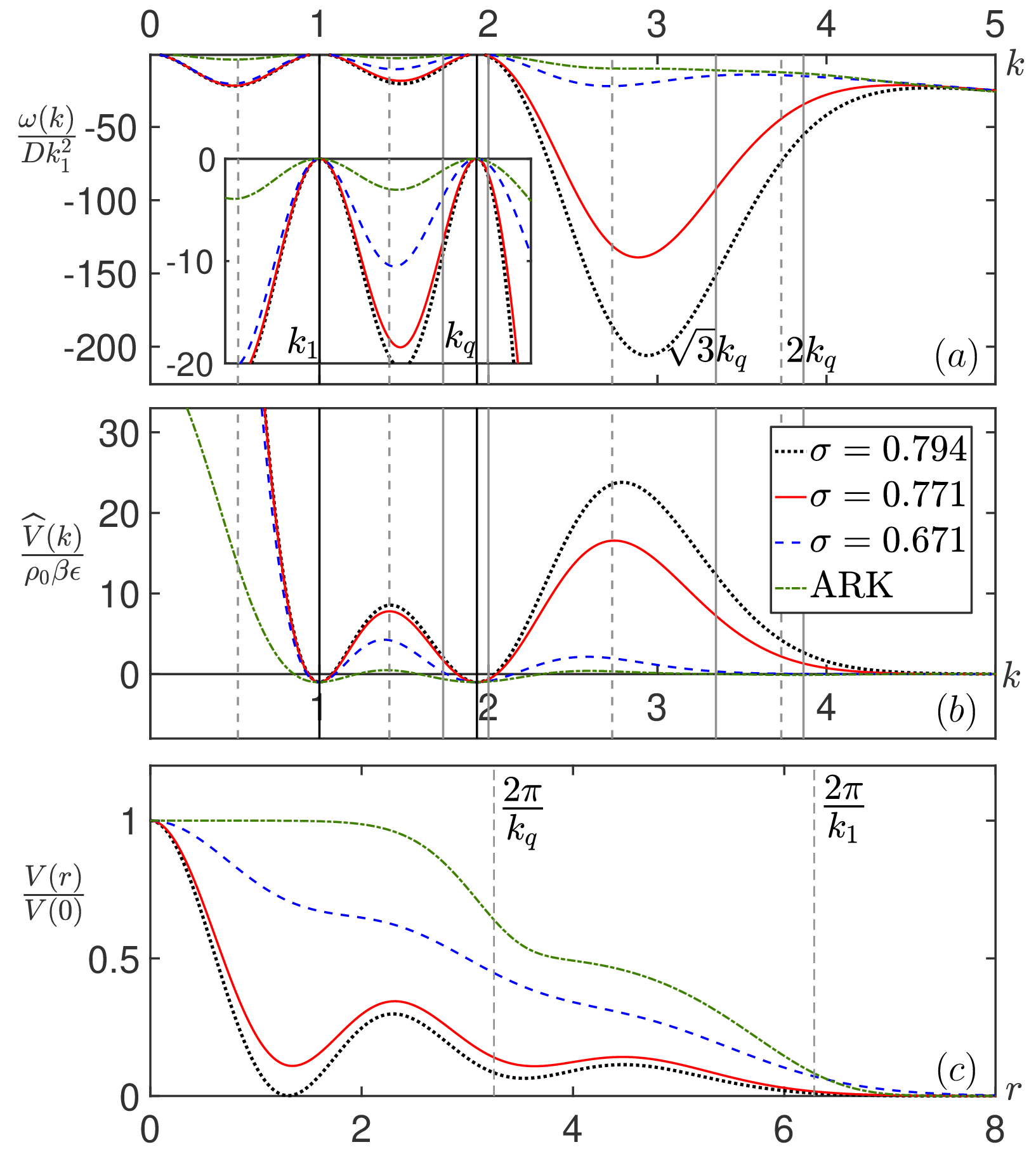 Figure 1
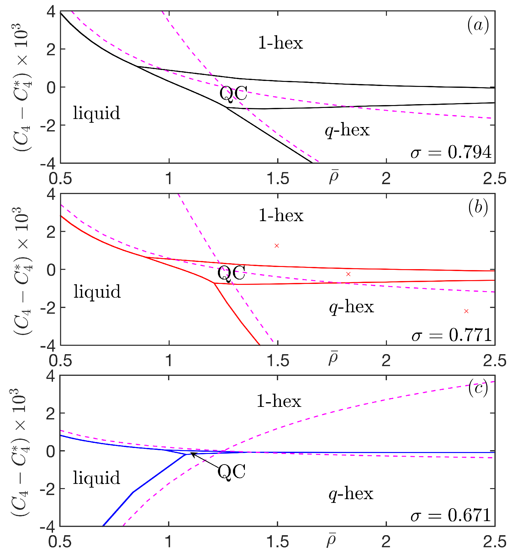 Figure 2
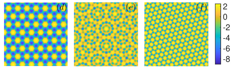 Figure 3
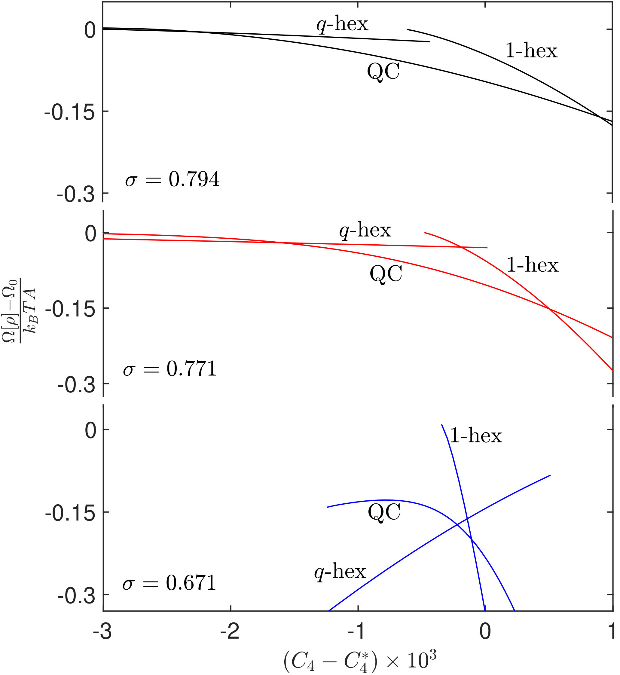 Figure 4
| 0.794 | 1.350 | 1.794 | 0.7224 | 0.08368 | 0.003117 |
| 0.771 | 1.000 | 1.095 | 0.4397 | 0.04927 | 0.001831 |
| 0.671 | 0.3949 | 0.04485 | 0.03689 | 0.003342 | 0.0001449 |
Peer Reviews
No public reviews on file for this paper yet. If you reviewed it on a platform where reviews are public (OpenReview, ICLR, NeurIPS, ICML), you can paste yours below so the community can read it here.
Videos
No videos yet. Explain this paper in a talk, walkthrough, or lecture? Add one.
Which wavenumbers determine the thermodynamic stability of soft matter quasicrystals?
D.J. Ratliff
Department of Mathematical Sciences and Interdisciplinary Centre for Mathematical Modelling, Loughborough University, Loughborough, Leicestershire LE11 3TU, United Kingdom
A.J. Archer
Department of Mathematical Sciences and Interdisciplinary Centre for Mathematical Modelling, Loughborough University, Loughborough, Leicestershire LE11 3TU, United Kingdom
P. Subramanian
School of Mathematics, University of Leeds, Leeds LS2 9JT, United Kingdom
Mathematical Institute, University of Oxford, Oxford OX2 6GG, United Kingdom
A.M. Rucklidge
School of Mathematics, University of Leeds, Leeds LS2 9JT, United Kingdom
Abstract
For soft matter to form quasicrystals an important ingredient is to have two characteristic lengthscales in the interparticle interactions. To be more precise, for stable quasicrystals, periodic modulations of the local density distribution with two particular wavenumbers should be favored, and the ratio of these wavenumbers should be close to certain special values. So, for simple models, the answer to the title question is that only these two ingredients are needed. However, for more realistic models, where in principle all wavenumbers can be involved, other wavenumbers are also important, specifically those of the second and higher reciprocal lattice vectors. We identify features in the particle pair interaction potentials which can suppress or encourage density modes with wavenumbers associated with one of the regular crystalline orderings that compete with quasicrystals, enabling either the enhancement or suppression of quasicrystals in a generic class of systems.
Matter does not normally self-organise into quasicrystals (QCs). Regular crystalline packings are much more common in nature and some specific ingredients are required for QC formation, which is why the first QCs were not identified until 1982, in certain metallic alloys Shechtman et al. (1984). Subsequently, the seminal work in Refs. Lifshitz and Petrich (1997); Lifshitz and Diamant (2007) showed that normally a crucial element in QC formation, at least in soft matter, is the presence of two prominent wavenumbers in the linear response behavior to periodic modulations of the particle density distribution. This is equivalent to having two prominent peaks in the static structure factor or in the dispersion relation Archer et al. (2013, 2015). In soft matter systems, the effective interactions between molecules and aggregations of molecules (generically referred to here as particles) can be tuned to exhibit the two specific required lengthscales and thus form QCs. Such systems include block copolymers and dendrimers Zeng et al. (2004); Hayashida et al. (2007); Fischer et al. (2011); Glotzer and Engel (2011); Iacovella et al. (2011); Zhang and Bates (2012); Lee et al. (2014); Gillard et al. (2016); Yue et al. (2016); Huang et al. (2018), certain anisotropic particles Haji-Akbari et al. (2009, 2011); Dontabhaktuni et al. (2014), nanoparticles Talapin et al. (2009); Ye et al. (2017) and mesoporous silica Xiao et al. (2012).
Some of our understanding of how and why QCs can form has come from studies of particle based computer simulation models – see for example Engel and Trebin (2007); Dotera et al. (2014); Engel et al. (2015); Martinsons and Schmiedeberg (2018); Gemeinhardt et al. (2019). Another source of important insights has been continuum theories for the density distribution. The earliest of these consist of generalised Landau-type order-parameter theories Lifshitz and Petrich (1997); Lifshitz and Diamant (2007); Achim et al. (2014); Jiang and Zhang (2014); Jiang et al. (2015); Subramanian et al. (2016); Schmiedeberg et al. (2017); Jiang et al. (2017); Subramanian et al. (2018); Savitz et al. (2018). More recently, classical density functional theory (DFT) Hansen and McDonald (2013); Evans (1979, 1992) in conjunction with its dynamical extension DDFT Marconi and Tarazona (2000); Archer and Evans (2004); Archer and Rauscher (2004) has been utilised. DFT is a statistical mechanical theory for the distribution of the average particle number density that takes as input the particle pair interaction potentials, and so bridges between particle based and Landau-type continuum theory approaches. The DFT results for QC forming systems Barkan et al. (2011); Archer et al. (2013); Barkan et al. (2014); Archer et al. (2015); Walters et al. (2018) clearly demonstrate how the crucial pair of prominent wavenumbers are connected to the length and energy scales present in the pair potentials.
Whilst the ratio between the two lengthscales is important, it can be seen that this is not the whole story if one compares the phase behavior of systems with the pair potential of Ref. Barkan et al. (2014) (phase diagrams are calculated below) with the phase behavior of the core-shoulder soft potential system of Refs. Archer et al. (2013, 2015). We refer to these two as the BEL and ARK models respectively. In the ARK model, QCs are never the thermodynamic equilibrium phase, i.e., the state which is the global minimum of the free energy, and they only form in this system for subtle dynamical reasons Archer et al. (2013, 2015). In contrast, QCs can be the thermodynamic equilibrium for the BEL model. This is despite the fact that the parameters in both the BEL and ARK models are chosen so that both systems have identical growth rates at the two critical wavenumbers and , so that density fluctuations with these two wavenumbers are promoted equally in the two different systems. This raises the important question: what feature(s) do BEL-type systems have that enables QCs to be thermodynamically stable, that ARK-type systems do not have? Or, relating to the title question, why is it not enough to consider just these two wavenumbers?
The answer to this question is that one must also consider the properties of the dispersion relation at certain other wavenumbers . For example, in two dimensions (2D), hexagonal crystals are built up from six modes at to one another with equal (single) wavenumber . They are stabilized by nonlinear coupling between these modes and modes with wavenumbers such as , and , which are generated by vector sums of the original six. The resulting wavevectors are the hexagonal reciprocal lattice vectors (RLVs). More generally, with two wavenumbers, more complex structures can form and involve larger sets of RLVs. The properties of modes with these vectors, in particular their decay rates , must be known in order to predict which structures have the lowest free energy.
We illustrate this fundamental understanding by developing a class of model systems with pair potentials which have identical growth rates at and , but are different in a controllable manner at the RLV wavenumbers. By changing the dispersion relation at these wavenumbers, we are able either to enhance or suppress the stability of QCs.
Whilst it is not a priori obvious that soft matter freezing might be related to Faraday waves, it turns out that a surprisingly large amount of the mathematics of Faraday wave pattern formation can be applied to the soft matter systems of interest here, including the understanding of QC stability Lifshitz and Petrich (1997); Edwards and Fauve (1994); Zhang and Viñals (1997); Silber et al. (2000); Porter et al. (2004); Porter and Silber (2004); Rucklidge and Silber (2009); Skeldon and Guidoboni (2007); Skeldon and Rucklidge (2015). Faraday waves are standing waves on the surface of viscous liquid layers that arise when the liquid is subjected to strong enough vertical vibrations Miles and Henderson (1990). In some circumstances, Faraday wave experiments exhibit spatially complex patterns such as twelvefold quasipatterns at parameters where two lengthscales in the correct ratio are excited or weakly damped Edwards and Fauve (1994); Gollub (1995); Besson et al. (1996); Arbell and Fineberg (2002); Kudrolli et al. (1998); Ding and Umbanhowar (2006); Rucklidge et al. (2012); Skeldon and Rucklidge (2015). A major conclusion from this body of work is that understanding spatially complex patterns in Faraday waves requires the consideration of not only the primary waves in the pattern but also the contributions from the RLV waves. These RLV contributions are strongly influenced by the damping rate at each wavenumber. We demonstrate here that analogous mechanisms operate in the coupling between soft matter density modulations at different wavenumbers, helping to identify features in the pair potentials that can be tuned to control the extent to which the QCs are stabilized.
For a system of interacting particles free of any external forces, the equilibrium density distribution is given by the minimum of the grand potential functional Hansen and McDonald (2013); Evans (1979, 1992)
[TABLE]
where is the thermal de-Broglie wavelength, is Boltzmann’s constant, is the temperature and is the chemical potential. In 2D, we have and . We illustrate the main ideas of this letter in 2D, but they equally apply in 3D. The first term in Eq. (1) is the entropic ideal-gas contribution to the Helmholtz free energy, while the second term is the excess contribution, which arises from the interactions between particles. The random phase approximation (RPA) Hansen and McDonald (2013); Likos (2001)
[TABLE]
turns out to be remarkably accurate for soft particles interacting pairwise via potentials , which are finite for all values of the separation distance between the particles Likos (2001) and so is used here. Equilibrium density profiles minimize (1) and so satisfy the Euler–Lagrange equation . In the liquid state, the density is uniform, whilst in the crystal and QC phases the profiles are nonuniform, typically with sharp peaks.
An understanding of how the thermodynamic equilibrium structures are selected comes from rewriting Eq. (2) in Fourier space:
[TABLE]
where is the Fourier transform of the density profile and is similarly defined as the Fourier transform of . We observe that density modes with wavenumbers at the minima of minimise the above integral, whereas those with wavenumbers away from these values make a larger contribution to and so are favored less. In other words, quantifies the energetic penalty for having modes with wavenumber in the density profile. Of course, the entropic ideal-gas term in (1) also makes an important contribution. This is particularly true near to melting, which is where the soft QCs discussed here exist.
Assuming that the particles have overdamped Brownian equations of motion, the nonequilibrium dynamics of the density distribution is given by DDFT Marconi and Tarazona (2000); Archer and Evans (2004); Archer and Rauscher (2004)
[TABLE]
where is time and is a mobility coefficient. The stability of a uniform liquid state of density to small amplitude perturbations can be found by a standard normal mode approach Archer and Evans (2004); Archer et al. (2012, 2013, 2015), which gives the linear dispersion relation for the growth (or decay) rate associated with modes of wavenumber ,
[TABLE]
where is the diffusion coefficient and . In (5) the first term () stems from the ideal-gas contribution and is entropic in origin, whilst the second term () is the energetic contribution. The liquid is dynamically stable when for all , but becomes unstable at critical wavenumber(s) if at a local maximum. This can only happen if for some range of Likos et al. (2007), and then the instability occurs through increasing or decreasing . For the class of two lengthscale systems here, there are two maxima in , at and . The ratio between these is important for determining the structures formed, but as we now show, other wavenumbers in the reciprocal lattice are important too.
We demonstrate this by modifying a pair potential in such a way that remains fixed at and but changes everywhere else, strongly affecting which structures minimize Eq. (1) and so are the thermodynamic equilibria. We use the form of the BEL pair potential Barkan et al. (2014):
[TABLE]
Throughout we set and the remaining parameters have values chosen so that the dispersion relation has two maxima at and [minima in ], but varies significantly for other values. We choose three sets of parameter values, given in Table 1, in order to enhance or reduce the energetic cost at other RLV wavenumbers. The middle set, with , are the values originally used in Ref. Barkan et al. (2014). The resulting dispersion relations, Fourier transforms of the pair potentials and the potentials in real space are displayed in Fig. 1.
From Fig. 1, we see that decreasing results in being more damped at larger values and thus leads to a lower energetic penalty [see Eq. (3)] at the hexagonal RLV wavenumbers of and , i.e., at the wavenumbers , , , , which are marked as vertical gray lines in Fig. 1 and 1. In contrast, increasing leads to a higher penalty at the hexagonal RLV wavenumbers. There are corresponding changes to the decay rates (Fig. 1). The important QC RLV wavenumbers are , , and (dashed gray lines), and there are of course also changes in the value of at these wavenumbers as is varied. However, on decreasing the biggest fractional change in occurs at wavenumber , where decreases by 90% going from to , whilst the change at is 88% and at all other key wavenumbers the fractional change is significantly smaller. Therefore, hexagons with wavenumber (-hex) should be stabilized more than QCs by the decrease in , which we confirm below by calculating free energies and phase diagrams – see Figs. 2 and 3.
We also display in Fig. 1 the ARK model pair potential and corresponding and . We choose the parameter values so that the system is identical to that studied in Refs. Archer et al. (2013, 2015), i.e., with and , where the phase diagram was also determined. Here we rescale the core and shoulder radii and by choosing , so that the critical wavenumbers are at and as in the three chosen BEL potentials (6). This rescaling does not in any way change the phase behavior.
Figure 1 illustrates how varying the parameters changes the architecture of the potentials in physical space. Increasing (together with changes to the other parameters) leads to oscillations in the BEL potential becoming accentuated, to the extent that the first minimum at comes close to zero in the case. On the other hand, the opposite changes smooth the oscillations, to the point where it becomes hard, in real space, to discern more than one length scale. The BEL potential with bears some resemblance to the the ARK potential.
In Fig. 2 we display equilibrium phase diagrams, computed by varying and , and minimising the grand potential (1) via Picard iteration Roth (2010); Archer et al. (2013). The top three panels are for the three chosen BEL potentials, and show the equilibrium phase as a function of average density and . Here, is the value of for simultaneous marginal stability, as given in Table 1. Varying away from means that the maxima in are no longer at the same value, shifting the preference to one or other length scale Walters et al. (2018). Typical examples of the density profiles obtained are displayed along the bottom of Fig. 2.
Figure 3 shows examples of the grand potential per unit area (relative to the value for the liquid ) as a function of at constant . In these plots, the thermodynamic equilibrium phase is that with the lowest value of for the given value of . The crossing points of the different branches in each case give the phase boundaries displayed in Fig. 2.
The size of the region where QCs are stable in each phase diagram in Fig. 2 come from the changes to the potentials shown in Fig. 1. Case () with the larger has QCs as the thermodynamic equilibrium over a much larger region of the phase diagram than (), with the smaller , where they are almost completely suppressed. In the ARK phase diagram displayed in Archer et al. (2013, 2015), QCs are completely absent. The reason for these significant changes is that decreasing and thus making less negative away from and (see Fig. 1) benefits all phases that incorporate other wavenumbers, but benefits most the -hex crystals, as discussed above. In common with Faraday waves, wavenumbers that are less strongly damped play a more prominent role in selecting the final state Newell and Pomeau (1993). Of course, determining the thermodynamic equilibrium involves a nonlinear balance between contributions from all RLV wavenumbers, but our results in Figs. 2 and 3 are consistent with this intuition from Faraday waves.
A simplification that is made in some other models is to introduce a coefficient (the parameter in Jiang and Zhang (2014); Jiang et al. (2015); Savitz et al. (2018); Jiang and Si (2019) or in Jiang et al. (2017)) which effectively sends for all wavenumbers , as . This limit of perfect lengthscale selectivity makes the resulting pair interaction potentials less physically realisable. The present approach does not rely on this simplification and is therefore more relevant to elucidating QC formation in soft matter at finite temperatures.
To conclude, we return to the title question: As Refs. Lifshitz and Petrich (1997); Lifshitz and Diamant (2007) showed and subsequent work confirmed, two wavenumbers and having a specific ratio are required for quasicrystals to be stable, i.e., a local minimum of the grand potential. However, what we have shown here is that for QCs to be the thermodynamic equilibrium, one must also consider the RLV wavenumbers of all competing crystal structures. Moreover, examining the value of the dispersion relation at these other RLV wavenumbers helps anticipate the outcome of the competition between QCs and other crystal structures.
Acknowledgements
This work was supported in part by a L’Oréal UK and Ireland Fellowship for Women in Science (PS), by the EPSRC under grants EP/P015689/1 (AJA, DR) and EP/P015611/1 (AMR), and by the Leverhulme Trust (RF-2018-449/9, AMR). DJR would like to thank Ron Lifshitz, Sam Savitz and Ken Elder for various helpful discussions during the formulation of this paper.
The reference list from the paper itself. Each links out to its DOI / PubMed record.
- 1Shechtman et al. (1984) D. Shechtman, I. Blech, D. Gratias, and J.W. Cahn, “Metallic phase with long-range orientational order and no translational symmetry,” Phys. Rev. Lett. 53 , 1951–1953 (1984).
- 2Lifshitz and Petrich (1997) R. Lifshitz and D.M. Petrich, “Theoretical model for Faraday waves with multiple-frequency forcing,” Phys. Rev. Lett. 79 , 1261–1264 (1997).
- 3Lifshitz and Diamant (2007) R. Lifshitz and H. Diamant, “Soft quasicrystals – Why are they stable?” Philos. Mag. 87 , 3021–3030 (2007).
- 4Archer et al. (2013) A.J. Archer, A.M. Rucklidge, and E. Knobloch, “Quasicrystalline order and a crystal-liquid state in a soft-core fluid,” Phys. Rev. Lett. 111 , 165501 (2013).
- 5Archer et al. (2015) A.J. Archer, A.M. Rucklidge, and E. Knobloch, “Soft-core particles freezing to form a quasicrystal and a crystal-liquid phase,” Phys. Rev. E 92 , 012324 (2015).
- 6Zeng et al. (2004) X. Zeng, G. Ungar, Y. Liu, V. Percec, A.E. Dulcey, and J.K. Hobbs, “Supramolecular dendritic liquid quasicrystals,” Nature 428 , 157–160 (2004).
- 7Hayashida et al. (2007) K. Hayashida, T. Dotera, A. Takano, and Y. Matsushita, “Polymeric quasicrystal: Mesoscopic quasicrystalline tiling in A B C 𝐴 𝐵 𝐶 ABC star polymers,” Phys. Rev. Lett. 98 , 195502 (2007).
- 8Fischer et al. (2011) S. Fischer, A. Exner, K. Zielske, J. Perlich, S. Deloudi, W. Steurer, P. Lindner, and S. Förster, “Colloidal quasicrystals with 12-fold and 18-fold diffraction symmetry,” PNAS 108 , 1810–1814 (2011).