Peaked and low action solutions of NLS equations on graphs with terminal edges
Simone Dovetta, Marco Ghimenti, Anna Maria Micheletti, Angela Pistoia

TL;DR
This paper studies the nonlinear Schrödinger equation on graphs with terminal edges, describing low action solutions concentrating on edges and constructing multi-peaked solutions at high frequencies.
Contribution
It introduces a profile description for low action solutions and develops a Ljapunov-Schmidt reduction to construct multi-peaked solutions on graphs with terminal edges.
Findings
Low action solutions concentrate on terminal edges.
Existence of multi-peaked solutions at large frequencies.
Solutions resemble rescaled real-line solutions.
Abstract
We consider the nonlinear Schr\"odinger equation with focusing power-type nonlinearity on compact graphs with at least one terminal edge, i.e. an edge ending with a vertex of degree 1. On the one hand, we introduce the associated action functional and we provide a profile description of positive low action solutions at large frequencies, showing that they concentrate on one terminal edge, where they coincide with suitable rescaling of the unique solution to the corresponding problem on the real line. On the other hand, a Ljapunov-Schmidt reduction procedure is performed to construct one-peaked and multipeaked positive solutions with sufficiently large frequency, exploiting the presence of one or more terminal edges.
Click any figure to enlarge with its caption.
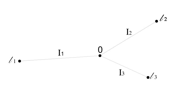 Figure 2
Peer Reviews
No public reviews on file for this paper yet. If you reviewed it on a platform where reviews are public (OpenReview, ICLR, NeurIPS, ICML), you can paste yours below so the community can read it here.
Videos
No videos yet. Explain this paper in a talk, walkthrough, or lecture? Add one.
Peaked and low action solutions of NLS equations
on graphs with terminal edges
S. Dovetta, M. Ghimenti, A. M. Micheletti, A. Pistoia
Abstract
We consider the nonlinear Schrödinger equation with focusing power–type nonlinearity on compact graphs with at least one terminal edge, i.e. an edge ending with a vertex of degree 1. On the one hand, we introduce the associated action functional and we provide a profile description of positive low action solutions at large frequencies, showing that they concentrate on one terminal edge, where they coincide with suitable rescaling of the unique solution to the corresponding problem on the real line. On the other hand, a Ljapunov–Schmidt reduction procedure is performed to construct one–peaked and multipeaked positive solutions with sufficiently large frequency, exploiting the presence of one or more terminal edges.
1 Introduction
Metric graphs (or networks) are locally one–dimensional structures built of several intervals, the edges, glued together at some of their endpoints, the vertices. The specific way in which the edges are joined determines the topology of the graph. When a differential operator acting on functions supported on the graph is defined, we also speak of quantum graphs.
The birth of quantum graphs can be traced back to the first half of the Fifties of the last century [32], when the spectral analysis of Schrödinger operators on a network modelling molecular bonds has been proposed to investigate the behaviour of valence electrons in a naphthalene molecule. Since then, graphs have been assumed to provide a meaningful tool to model the dynamics of systems confined to ramified domains.
Despite the fact that, in general, to rigorously justify the graph approximation is still an open problem (see for instance [20, 26] as well as [12, 18] and references therein), the last decades have been witnessing a renewed interest in the theory of quantum graphs, mainly driven by a wide variety of applications, e.g. Josephson junctions, propagations of signals, nonlinear optics and so on. Among these, the most prominent topic is probably given by the theory of Bose–Einstein condensates, that contributes to gather the focus on nonlinear Schrödinger (NLS) equations as
[TABLE]
Particularly, many efforts have been profuse in the analysis of standing waves of (1), i.e. solutions of the form , for suitable and solving the associated stationary equation
[TABLE]
First investigations have been developed on specific examples of graphs with half–lines, such as star graphs (see for instance [1, 2, 28]) and the tadpole graph, [29]. Later, the problem has been addressed on general non–compact graphs with half–lines, for which a quite well–established theory of existence of standing waves is nowadays available (see the series of works [5, 6, 7] for the case of the nonlinearity extended to the whole graph, and [16, 17, 33, 34, 35] for the counterpart with nonlinearities restricted to the compact core). Broadening the discussion, several results have been accomplished also on compact graphs [13, 14, 25] and periodic graphs [3, 4, 15, 30, 31]. Furthermore, similar investigations have been recently initiated on different families of nonlinear equations too, i.e. nonlinear KdV equation, [27], and nonlinear Dirac equation [10, 11].
From the standpoint of Critical Point Theory, solutions of (2) can be identified at least in two different ways. On the one hand, one can search for critical points of the energy functional
[TABLE]
in the constrained space of functions with prescribed mass , that is
[TABLE]
This is for instance the general framework of [5, 6, 7] and related works, where it has been shown that the problem is sensitive both to topological and metric properties of the graph.
On the other hand, given , one can look for unconstrained critical points of the action functional
[TABLE]
This approach has been exploited in [30] in the case of periodic graphs, and in [21, 22, 23] on star–graphs. Precisely, in [30], minimization on a generalized Nehari manifold is performed to show existence of least action solutions, whereas in [21, 22, 23] the focus is set on stability properties of specific critical points of the functional.
Our work here fits in the investigation of the action functional (3). Let us now describe informally the main results of the paper, redirecting to the next section for the precise setting and statements.
In what follows, we restrict our attention to compact graphs with at least one terminal edge, that is an edge ending with a vertex of degree 1. Our aim is twofold.
On one side, it is easy to show that a solution of (2) can always be found minimizing the action on a suitable Nehari manifold. Hence, we concentrate on low action positive solutions and, given large enough, we provide a profile description for such states. Specifically, we show that these solutions are strongly affected by the presence of a terminal edge, as it can be proved that they reach their maximum at a vertex of degree 1, whereas they are small in some norm outside of the corresponding terminal edge (Theorem 1).
On the other side, as soon as is sufficiently large, a Ljapunov–Schmidt reduction procedure is performed. Exploiting the topological assumption ensuring at least a terminal edge, we construct one–peaked (Theorem 2) and multipeaked (Theorem 3) solutions to (2), i.e. solutions with one or more maximum points at the vertices of degree 1, respectively, and negligibly small on the rest of the graph.
The existence of such highly concentrated states testifies the dependence of the problem on the topology of the underlying graphs, which is a common feature of these kind of problems on graphs (just to name an example in the framework of compact graphs, the role of terminal edges in existence issues for the mass–constrained case has been pointed out in [14]).
Let us highlight that several perspectives can be raised following up the aforementioned results. It is for instance unclear if functions sharing the minimal action can be further characterized, and if the metric of affects such minimizers. In the case of multiple terminal edges, we expect solutions of least action to attain their peak on the longest among these edges, but up to now we are not able to provide a proof of this conjecture.
Another natural question concerns the possibility of adapting our construction to graphs without terminal edges, exhibiting states with peaks in the interior of any given edge. With respect to this, we believe that the profile description of low action solutions as given in Theorem 1 generalizes straightforwardly, leading to a similar result for graphs with no terminal edges and solutions concentrated on an internal edge. Conversely, it seems to us that further work might be necessary for the Ljapunov–Schmidt scheme of Theorems 2–3. Indeed, it is not clear what suitable model function has to be considered in the absence of terminal edges, so that we expect nontrivial modifications of the argument to be required so to build peaked solutions with maximum points inside a general edge.
Finally, it remains an open problem to understand whether a profile description analogous to the one in Theorem 1 can be given when we minimize the energy functional under a mass constraint.We notice that, in the context of mass–constrained critical points, solutions attaining their maximum only inside a given edge have been constructed in [8], provided the mass is sufficiently large. In that paper, such existence result is achieved through the analysis of a doubly–constrained minimization problem. We wonder whether the methods we introduce in the present work could be adapted to recover and generalize those conclusions.
The paper is organised as follows. In Section 2 we recall some known facts and we state in details our main results. Section 3 is devoted to the profile description of low action solutions, developing the proof of Theorem 1, whereas Section 4 carries on the construction of peaked solutions as in Theorems 2–3.
2 Setting and main results
Before going further, let us briefly recall some definitions and some notation about metric graphs (for a standard reference see for instance the monograph [9]).
Throughout the paper, denotes a compact graph, i.e. the union of a finite number of vertices and edges , each one identified with an interval of finite length . The degree of a vertex is the number of edges entering it.
In what follows, we always assume that has at least one terminal edge, that is an edge ending with a vertex of degree 1.
A function supported on can be viewed as a bunch of functions where
[TABLE]
and, since the graph inherits the metric from its edges, we can easily define the Lebesgue space of functions such that
[TABLE]
A continuous function on is a function which is continuous on every edge and such that, if two edges and meet at a vertex , then and have the same value at v. We can also define the Sobolev space as follows:
[TABLE]
endowed with the norm
[TABLE]
Finally, the following Kirchhoff condition is considered at the vertices of
[TABLE]
Here, the symbol indicates every edge incident at v, and we use the convention that
[TABLE]
according to whether the coordinate is equal to [math] or at .
We want to study the positive solutions of the problem
[TABLE]
on a graph with terminal edges. Here and are given. Since , we endow with the following equivalent scalar product
[TABLE]
From now on, unless otherwise specified, we will always consider this product (and its related norm ) as the scalar product (and the norm) on
In order to find positive solutions of (4), we modify the action functional considering
[TABLE]
In fact, any critical point of is a solution of
[TABLE]
and, of course any positive solution of (4) is also a solution of (6). One can prove also that any nontrivial solution of (6) is a positive solution of (4), so any nontrivial critical point of is a positive solution of (4). To do that, it is sufficient to show that any solution of (6) is strictly positive. We know that as a minimum point . By contradiction, let us suppose that . If lies in the interior of some edge, then
[TABLE]
so and by the Cauchy theorem on the whole edge. Then, by Kirchhoff node condition we can prove that on , which is a contradiction. On the other hand, if coincides with a terminal vertex, we have that either or , and , and cannot be a minimum point. If coincides with and internal vertex, a similar argument applies and we get the proof.
Now, for every , let
[TABLE]
be the renormalized action functional, and consider the associated Nehari manifold
[TABLE]
It is standard to prove that is a natural constraint, i.e. that any nontrivial solution of (4) is a critical point of on .
Finally, we recall some useful features of a similar problem on the whole line , which provides the model functions to construct solutions of problem (4).
Let us consider
[TABLE]
It is well known (see [24]) that this equation admits a unique -up to translations- solution in which has the explicit form
[TABLE]
We set (see Section 3).
Notice that uniqueness of solution of (8) can be easily recovered when the equation is set in (we refer to [24] for the standard argument that can be straightforwardly adapted here). In this case any solution in has the form , where is a suitable translation.
The next theorem gives, for a sufficiently large , a profile description of low action solutions of (4). In particular these solutions have a unique peak at a vertex of degree 1, they are similar to a suitable rescaling of on this edge and negligible in norm on the rest of the graph.
Theorem 1**.**
Let be a compact graph with at least one terminal edge and . Let and let, for any , be a positive solution of (4) with . Then, up to subsequence, has a unique maximum point located in a terminal vertex v. Moreover, denoting by the terminal edge where attains its maximum (with the convention that the degree 1 vertex v concides with [math]) we have that, while
. 2. 2.
* weakly in and strongly in , in and in for all . Here is a cut off function.* 3. 3.
** 4. 4.
For every and every , there exist two constants , depending on but independent from , such that
[TABLE]
We point out that the assumption is consistent, as the sets of solutions fulfilling it is actually not empty (see Section 3 and Corollary 4).
Reversing the perspective, whenever has at least a vertex of degree 1 and again for large , it is possible to construct one-peaked solutions to problem (4), using the function as a model, and, if has several terminal edges, then it is possible to construct multipeaked solution. This is what is stated in the following two theorems.
Theorem 2**.**
Let be a compact graph with a vertex with degree and . Denote by the terminal edge ending at , with the convention that coincides with 0. Then, provided is sufficiently large, there exists a solution of (4) with a single peak at , i.e. of the form
[TABLE]
with
[TABLE]
where is a smooth cut–off function supported on , for some , and
[TABLE]
* being as in (9), and*
[TABLE]
for every . Furthermore,
[TABLE]
Theorem 3**.**
Let be a compact graph with vertices with degree and . Choose vertices of degree with . Let also denote the terminal edge ending at , with the convention that coincides with 0. Then, provided is sufficiently large, there exists a -peaked solution of (4) with a single peak at any vertex , , i.e. of the form
[TABLE]
with
[TABLE]
where is a smooth cut–off function supported on , for some , and
[TABLE]
* being as in (9), and*
[TABLE]
for every . Furthermore,
[TABLE]
In Section 4 we will show this construction based on the Ljapunov–Schmidt finite dimensional reduction. Again this procedure is possible for every , and the link between and is explicit. This gives also another interpretation of -critical exponent .
Remark 2.1*.*
A further observation about one-peaked solutions is possible. Given a sequence , let, be the corresponding one-peaked solution obtained by Theorem 2 for any . The sequence fulfills the hypothesis of Theorem 1, so it inherits all the properties given by Theorem 1: the exact location of the unique maximum point, the decreasing monotonicity, the decay rate and so on.
2.1 Notations
Herafter we will use the following recurrent notations.
- •
is the ball centered at with radius . We use the same notation either if or . In the last case, if we intend . Finally, .
- •
is a smooth cut–off function such that when and outside a ball of radius . When no ambiguity is possible we will omit the subscript .
- •
is the characteristic function of .
- •
With abuse of notation we often identify an edge with , being the lenght of the edge. When the edge is a terminal one, the vertex v of degree will be identified with [math].
- •
Given a vertex we will suppose w.l.o.g. that the degree of that vertex is either or strictly larger than . In fact, degree 2 vertices are indistinguishable from internal points.
3 Profile of low action solution
As stated in the previous sections, for any a solution of (4) can be obtained as a critical point of the action functional defined (see (7)) as
[TABLE]
on the Nehari manifold
[TABLE]
It is standard to prove that is a manifold and that the Palais-Smale condition holds on . Moreover, by (10) we have that
[TABLE]
The Nehari manifold is not empty, in fact, problem (4) admits a constant solution. Also, any solution that we will find in Section 4 belongs to .
One can easily prove that and, since Palais-Smale holds, that a non trivial minimizer exists. We set
[TABLE]
The one peaked solution of Section 4 allows also to estimate in term of the norm of the function defined in (9). Let us take a one-peaked solution given by Theorem 2. Let be the terminal edge where the peak is located, and suppose that the terminal vertex is in . We know that
[TABLE]
where , if and , if and for some fixed and
[TABLE]
Moreover for any positive . Thus we compute
[TABLE]
Set
[TABLE]
and we get
[TABLE]
This proves, also, that it is possible to find a sequence fulfilling the hypothesis of Theorem 1. We are able, by proving this theorem, to give an asymptotic profile description for a positive low action solution of problem (4).
Proof of Theorem 1.
The proof is divided in several steps.
Step 1: For large is not constant.
Indeed, if , then, by (4) necessarily Then
[TABLE]
where is the length of the graph. This contradicts .
Step 2: has a maximum point . Moreover, .
First, by standard regularity theory, we have that is a regular solution, that is, for any edge , . Since is not constant, and the graph is compact, has a global maximum point .
Now, if is on the interior of some edge , we have that and . Thus, by (4) we get , so .
If is assumed on a terminal vertex, again we have by Kirchhoff condition, so necessarily we have Thus again .
Finally suppose that is on a vertex of degree greater than
- Since is a maximum point, on any edge that insists on the vertex. Since, by (4), , we have At this point there exists at least an edge for which and we conclude as before.
Step 3: There exists a vertex such that, up to subsequences, while .
Suppose, by contradiction, that . Up to subsequences we can suppose that for all and we can identify . Thus we define
[TABLE]
The function belongs to , moreover
[TABLE]
So is bounded in , hence there exists such that weakly in and strongly in for any and in . We want to prove that is a nontrivial solution of (8).
Take . For large we have that the support of is contained in . We define a sequence of function (for large) as
[TABLE]
Since is a solution of (4) we have
[TABLE]
so by weak convergence on
[TABLE]
Since, by Step 2, then , so by convergence we can prove that . Thus, by uniqueness of solutions of (8) we have that . This leads to a contradiction. In fact, there exists such that
[TABLE]
and, since in there exists such that
[TABLE]
On the other hand, there exists such that, for it holds , so that if then and . So, for large we have
[TABLE]
So
[TABLE]
that contradicts our assumption, thus implying .
Step 4: Given v as in the previous step, we have .
Suppose, by contradiction, that . Define
[TABLE]
The function belongs to , and, in analogy with Step 3, we can prove that weakly in and strongly in for any and in . Given , for large we have that the support of is contained in and we can prove, as before, that is a nontrivial positive solution of (8) on , although we do not know its value at the origin. By uniqueness of solutions of (8) on , we have that for some suitable . Since for the maximum point of it holds , we have that has a maximum point in , so . At this point we can prove, similarly to Step 3, that there exists such that
[TABLE]
which contradicts our hypothesis.
Step 5: v coincides with an extremal vertex.
Suppose, by contradiction that v is a vertex with degree .
To simplify the notation, let the edges that intersect in v and let us suppose that for any , coordinates are defined on so that v coincides with , as shown in Figure 1. Suppose, also, that .
Choose and define, for , and
[TABLE]
As before, for any , is bounded in , and converges to some weakly in and strongly in for any and in .
Given any , there exists sufficiently large such that , so on we have that . Now, since solves (4), we have that
[TABLE]
and, since in , and by the arbitrariness of we have that in for all .
Finally is a nontrivial positive solution of (8) on , so
[TABLE]
We can prove that for all . In fact, we have that is a maximum point for , so is a maximum point for , so . Since, by Step 4, , we have that for convergence. Thus . Moreover for any by continuity of . Then also and, passing to the limit in , also that for any . Thus for all , since has a unique maximum. At this point, proceeding as before we have
[TABLE]
which leads us to a contradiction.
Step 6: has a unique maximum. Moreover, this maximum coincides with v.
By contradiction, suppose that has another maximum point . By the previous step, up to subsequences, it is possible to prove that there exists a terminal vertex w in such that . Moreover, one can check that w must coincide with v, otherwise .
Thus . At this point, let be as in (13) in Step 4
[TABLE]
and, setting , , we have
[TABLE]
By the previous steps it holds in , thus implying . On the other hand, in light of (14) we have which gives us a contradiction.
We can prove that exactly with the same argument, using the fact that since solves (4).
Step 7: in .
By Step 6, we have that is decreasing on . Now, given there exists an such that . Moreover, there exists such that, for , . So
[TABLE]
Step 8: Proof of Claim 1–2–3.
The proof of Claims 1 and 2 of the Theorem is a direct consequence of the previous steps. Moreover by Step 7
[TABLE]
and by a change of variable we obtain Claim 3.
Step 9: proof of Claim 4.
Let be given. First, we can repeat the argument of the previous steps to prove that has no local maximum point except for the extremal vertex. Therefore, is strictly decreasing on any edge of the graph.
Given again as in (13)
[TABLE]
by Step 7 we have in and, by definition, there exists a constant for which
[TABLE]
Now, fix and choose . Then there exists such that
[TABLE]
We have that
[TABLE]
indeed
[TABLE]
Now (16) implies, by rescaling, that
[TABLE]
so that, since for large, we have
[TABLE]
and, being strictly decreasing,
[TABLE]
Now, solves
[TABLE]
and, by (17) and since , there exists independent from such that
[TABLE]
Since it is well–known (see Lemma 2.4 of [19]) that, whenever
[TABLE]
there exist two constant , independent of , such that
[TABLE]
for every , we conclude. ∎
Corollary 4**.**
We have
[TABLE]
Proof.
By (11) we have . To prove the reverse inequality, assume by contradiction that there exists a sequence of solutions with , and, as in the proof of the previous theorem, we have
[TABLE]
being given by (13). Now, for any , there exists an such that
[TABLE]
and, since in there exists such that
[TABLE]
At this point we can proceed similarly to (12), obtaining
[TABLE]
The arbitrariness of provides the contradiction. ∎
4 Construction of peaked solutions
In order to perform the finite dimensional reduction, we have to linearize Problem (8) around the solution and to study the null space of the linearized problem, that is the set of solutions to the Neumann boundary value problem
[TABLE]
While the equation in has a one-dimensional space of solutions generated by , it is easy to show that problem (18) has only the trivial solution, due to the boundary condition.
This result can be expressed in a more general form for the so called star graphs, i.e. graphs that are union of half lines all connected to a same vertex . If is a star graph, the function
[TABLE]
is a solution of problem (4). Linearizing (4) around this solution we get the Kirchhoff boundary value problem
[TABLE]
and we can completely describe the space of solutions of (19).
We start looking for solutions of in and then we will consider the boundary conditions. The space of solutions in of is spanned by the solutions of the following two boundary value problems
[TABLE]
and
[TABLE]
We can extend -respectively by odd or even reflection- any solution of (20) and (21) to a solution of in . So we have that (21) has no solution in and . At this point a solution of (19), taking into account the Kirchhoff boundary condition is
[TABLE]
This implies that the solution of (19) form a dimensional linear space. This is in accordance to the case that is the half line, in which there are no solutions, and equivalent to for which the linear space is spanned by .
Remark 4.1*.*
When dealing with the time–dependent NLS equation
[TABLE]
it is well–known that linearizing around a solution leads to the following system of equations
[TABLE]
where and
[TABLE]
Note that the equation given by for the real part coincides with the one we derived in our discussion of the linearized problem. For the purposes of the forthcoming analysis, it is sufficient here to consider only this equation (for a wider discussion of the linearized problem on star graphs see for instance [22].)
Coming back to our original problem,let us consider, for a given compact graph , the compact immersion
[TABLE]
and define its adjoint map
[TABLE]
such that
[TABLE]
or equivalently
[TABLE]
4.1 One peaked solutions
We construct now a model profile for a solution which has a peak on the extremal vertex (the vertex of degree 1) of the first edge . We suppose, without loss of generality that corresponds to the coordinate . We define
[TABLE]
and, given a cut off function , with , we define
[TABLE]
and we search a solution of (4) of the form , being a small error in . To improve the readability of the paper, herafter we denote
[TABLE]
so a solution of (4) can be written as
[TABLE]
We define a linear operator
[TABLE]
and we recast equation (23) as
[TABLE]
where
[TABLE]
[TABLE]
The following result implies the invertibility of for sufficiently large.
Lemma 5**.**
There exists such that , it holds
[TABLE]
Proof.
We proceed by contradiction, assuming that there exist a sequence and a sequence of functions such that and
[TABLE]
By definition of we have
[TABLE]
that is
[TABLE]
and, set and we get
[TABLE]
Also, we have
[TABLE]
and, on the other hand,
[TABLE]
In light of (24) we have that for all , and, since outside the first edge , also that on . Thus
[TABLE]
and, since in and by (25), we have
[TABLE]
On the edge we consider the rescaling and we set
[TABLE]
Of course
[TABLE]
and, recalling the definition (22) of , and (24),
[TABLE]
where . Moreover it holds, for some constant ,
[TABLE]
in fact
[TABLE]
which is bounded by (25). Analogously
[TABLE]
By (27) we have that there exists a function defined on such that, fixed any ,
[TABLE]
We can show, indeed, that . Consider
[TABLE]
Since we have that thus admits a weak limit in . Also, on , so weakly in and .
Now, take a function , and take such that the support of is included in , so
[TABLE]
Integrating by parts the first term and passing to the limit we have that
[TABLE]
Since is arbitrary, we have that is a solution of (18), so . Moreover, extending by zero to the whole half line, we have , thus
[TABLE]
This leads to a contradiction in light of (26), in fact
[TABLE]
This concludes the proof. ∎
Proposition 6**.**
We have for any .
Proof.
Take . Then we have, by direct computation, that
[TABLE]
and Thus, multiplying (28) by , and integrating by parts we have
[TABLE]
By a change of variables, and since decays exponentially in , we have
[TABLE]
In the same way we can proceed for and , obtaining the claim. ∎
Proof of Theorem 2.
We look for a solution of (23) in the form , where is defined in (22). This corresponds to find a fixed point of the map
[TABLE]
We prove that is a contraction on for some positive . By Lemma 5, there exists such that
[TABLE]
By the mean value theorem and by the properties of there exists such that
[TABLE]
so, if is small enough, then also is small and we can find a constant such that
[TABLE]
In a similar way we can prove that, if is small enough, by Proposition 6
[TABLE]
Then there exists such that maps a ball of center [math] and radius in into itself and it is a contraction. So there exists a fixed point with norm .
At this point we proved that (4) has a one-peaked solution , with . To conclude the proof we compute the norm of the solution, that is
[TABLE]
which concludes the proof. ∎
4.2 Multipeaked solutions
We consider now a graph which has at least vertices of degree , and we construct a solution of (4) which has a positive peak on any vertex , . Without loss of generality we suppose that each vertex , lies on of the edge and that corresponds to the coordinate .
The strategy of the proof is similar to the previous one, so we only underline the differences. We define
[TABLE]
where
[TABLE]
and, is a cut off function which is on and [math] on and on every other edge , . Here .
It is clear that . As before, we search a solution of (4) of the form , being a small error in . We can prove the invertibility of the operator as following.
Lemma 7**.**
There exist such that , it holds
[TABLE]
Proof.
As before, we proceed by contradiction, assuming that there exist a sequence and a sequence of functions such that and
Setting and , we can prove as in Lemma 5 that solves equation (24) and that as . Since outside the first edges , we have
[TABLE]
This means that there is at least one edge such that
[TABLE]
Letting now , we can define the functions
[TABLE]
and we can repeat the argument of Lemma 5 to prove that as . This contradicts (31). ∎
Proposition 8**.**
We have for any .
Proof.
As in Proposition 6, we take , where is defined in (29). Then we find that solves the following differential equation
[TABLE]
which leads to the same conclusion of Proposition 6. ∎
Proof of Theorem 3.
The proof of this theorem is verbatim the proof of Theorem 2. ∎
The reference list from the paper itself. Each links out to its DOI / PubMed record.
- 1[1] Adami R., Cacciapuoti C., Finco D., Noja D., Variational properties and orbital stability of standing waves for NLS equation on a star graph , J. Differential Equations 257 , no. 10 (2014), 3738–3777.
- 2[2] Adami R., Cacciapuoti C., Finco D., Noja D., Constrained energy minimization and orbital stability for the NLS equation on a star graph , Ann. I. H. Poincaré – AN 31 (2014), 1289–1310.
- 3[3] Adami R., Dovetta S., One-dimensional versions of three-dimensional system: ground states for the NLS on the spatial grid , Rendiconti di Matematica e delle sue applicazioni, 39 7 (2018), 181–194.
- 4[4] Adami R., Dovetta S., Serra E., Tilli P., Dimensional crossover with a continuum of critical exponents for NLS on doubly periodic metric graphs , Anal. PDE, Vol. 12 (2019), No. 6, 1597–1612.
- 5[5] Adami R., Serra E., Tilli P., NLS ground states on graphs , Calc. Var. PDE 54 (2015), no. 1, 743–761.
- 6[6] Adami R., Serra E., Tilli P., Threshold phenomena and existence results for NLS ground states on metric graphs , J. Funct. Anal. 271 (2016), no. 1, 201–223.
- 7[7] Adami R., Serra E., Tilli P., Negative energy ground states for the L 2 superscript 𝐿 2 L^{2} –critical NLSE on metric graphs , Comm. Math. Phys. 352 (2017), no. 1, 387–406.
- 8[8] Adami R., Serra E., Tilli P., Multiple positive bound states for the subcritical NLS equation on metric graphs , Calc. Var. (2019) 58:5. https://doi.org/10.1007/s 00526-018-1461-4.