On exponential stabilization of nonholonomic systems with time-varying drift
Victoria Grushkovskaya, Alexander Zuyev

TL;DR
This paper develops a method for exponentially stabilizing a class of nonlinear control systems with time-varying drift using periodic feedback controls, ensuring stability under certain conditions.
Contribution
It introduces an explicit parametrization of periodic time-varying feedback controllers for stabilization of nonlinear systems with bounded drift, under a non-resonance assumption.
Findings
Controllers guarantee exponential stability when the period is sufficiently small
Method successfully stabilizes an underwater vehicle model
Method applied to stabilize a front-wheel drive car
Abstract
A class of nonlinear control-affine systems with bounded time-varying drift is considered. It is assumed that the control vector fields together with their iterated Lie brackets satisfy Hormander's condition in a neighborhood of the origin. Then the problem of exponential stabilization is treated by exploiting periodic time-varying feedback controls. An explicit parametrization of such controllers is proposed under a suitable non-resonance assumption. It is shown that these controllers ensure the exponential stability of the closed-loop system provided that the period is small enough. The proposed control design methodology is applied for the stabilization of an underwater vehicle model and a front-wheel drive car.
Click any figure to enlarge with its caption.
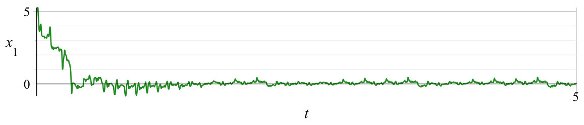 Figure 1
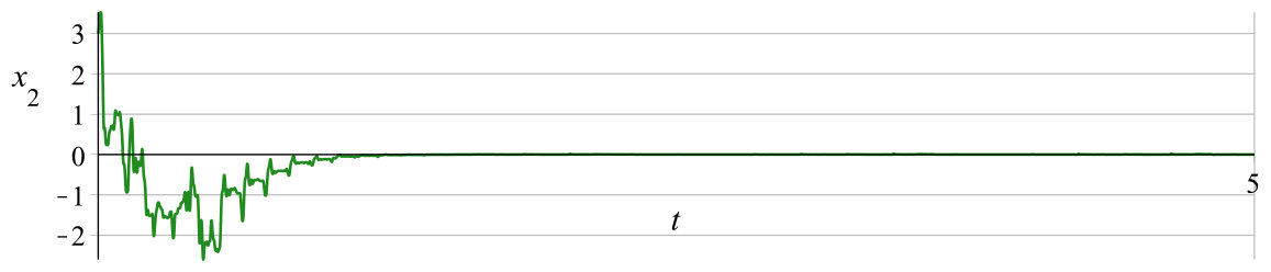 Figure 2
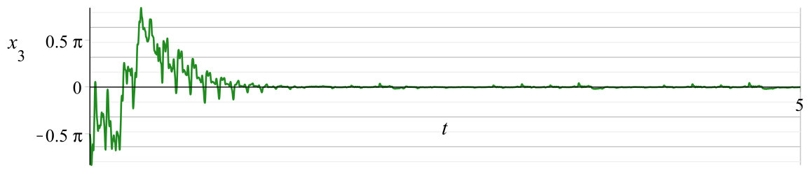 Figure 3
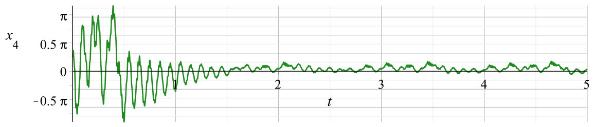 Figure 4
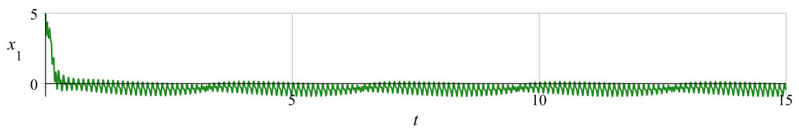 Figure 5
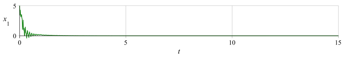 Figure 6
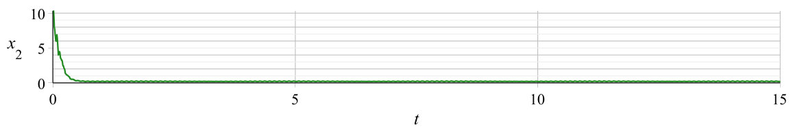 Figure 7
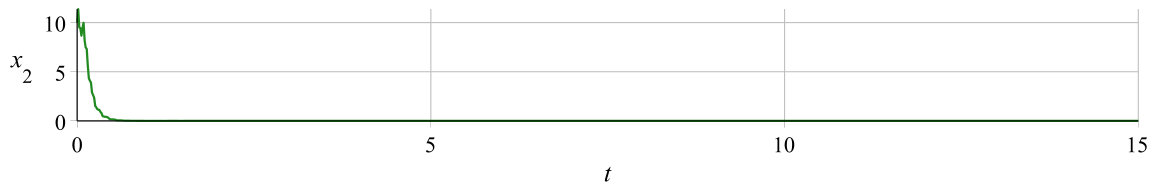 Figure 8
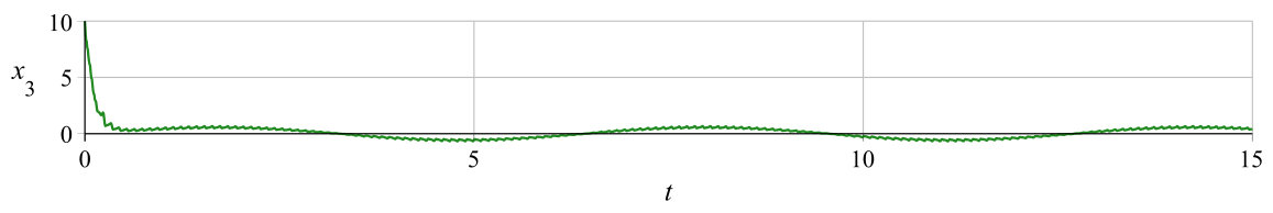 Figure 9
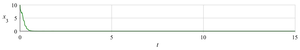 Figure 10
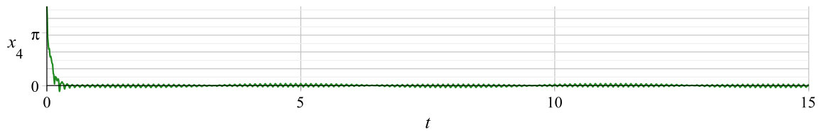 Figure 11
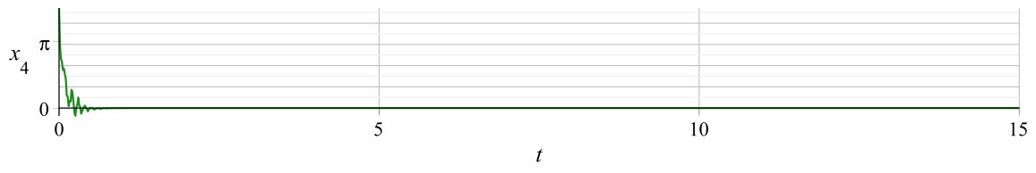 Figure 12
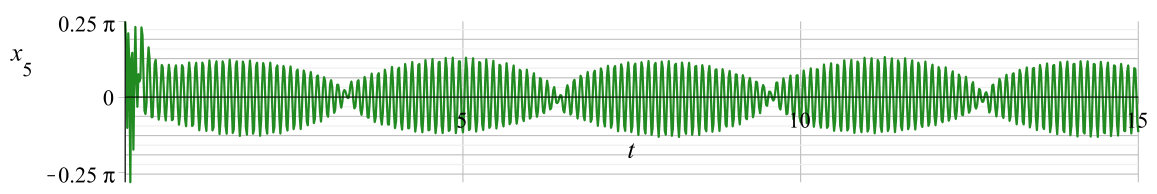 Figure 13
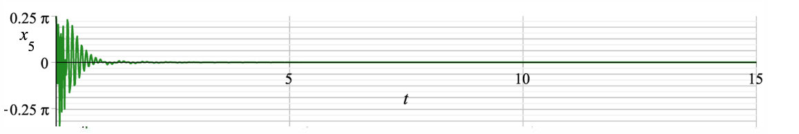 Figure 14
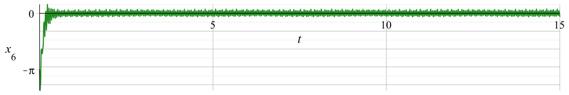 Figure 15
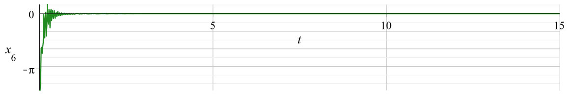 Figure 16
Peer Reviews
No public reviews on file for this paper yet. If you reviewed it on a platform where reviews are public (OpenReview, ICLR, NeurIPS, ICML), you can paste yours below so the community can read it here.
Videos
No videos yet. Explain this paper in a talk, walkthrough, or lecture? Add one.
On exponential stabilization of nonholonomic systems with time-varying drift††thanks:
This work is supported in part by the German Research Foundation (project GR 5293/1-1), the State Fund for Fundamental Research of Ukraine (project F78/206-2018), and NAS of Ukraine (budget program KPKBK 6541230).
1Institute of Mathematics, Julius Maximilian University of Würzburg, Germany [email protected]
2Max Planck Institute for Dynamics of Complex Technical Systems, Magdeburg, Germany [email protected]
3Institute of Applied Mathematics and Mechanics, National Academy of Sciences of Ukraine
Victoria Grushkovskaya1,3 and Alexander Zuyev2,3
Abstract
A class of nonlinear control-affine systems with bounded time-varying drift is considered. It is assumed that the control vector fields together with their iterated Lie brackets satisfy Hörmander’s condition in a neighborhood of the origin. Then the problem of exponential stabilization is treated by exploiting periodic time-varying feedback controls. An explicit parametrization of such controllers is proposed under a suitable non-resonance assumption. It is shown that these controllers ensure the exponential stability of the closed-loop system provided that the period is small enough. The proposed control design methodology is applied for the stabilization of an underwater vehicle model and a front-wheel drive car.
1 Introduction
The paper focuses on the stabilization problem for a class of nonholonomic systems in the control-affine form. As the number of control inputs in such systems can be significantly smaller than the dimension of the state vector, this causes certain challenges in control design. There exists a number of approaches which allow to stabilize control-linear nonholonomic systems (see, e.g., [6, 2, 18, 24], and references therein). However, the stabilization problem becomes even more complicated for control-affine systems with unstable drift terms. Controllability properties and motion planning problems of control-affine systems were discussed, e.g., in [7, 10, 19, 1, 14, 25]. While rather general results have been obtained for motion planning problems, stabilization of nonholonomic systems with drift is mainly studied for specific classes of systems (see, e.g., [16, 20, 4, 8, 21, 22, 9, 23], and [15, 17] for a survey). A more general class of control-affine systems was considered in [13, 17], where stabilizing controllers have been proposed under the assumption that the system is strongly controllable and can be approximated by a system with nilpotent Lie algebra, and that the drift term vanishes at the origin.
In this paper, we propose a class of control functions that stabilize the origin of an underactuated control-affine system with time-varying drift term. In general, we do not assume that the drift vanishes at the origin, which leads to the practical asymptotic stability of the corresponding closed-loop system. For a special class of drift terms vanishing at the origin, we show that the trajectories of the system exponentially tend to zero. We also do not involve the drift vector field in the controllability rank condition. In Section 2, we formulate the problem statement and present a novel stabilizability result as an the extension of the control design approach from ([24, 11]). Section 3 contains the proofs. Several examples are presented in Section 4.
2 Main results
2.1 Problem statement
Consider a system
[TABLE]
where is the state, is the control, describe the system dynamics, and is the drift term related to the system dynamics or to disturbances. In this paper, we propose a family of control laws for stabilizing the origin of system (1) under the assumption that the vector fields together with their first- and second-order Lie brackets span the whole -dimensional space, and the drift satisfies certain boundedness assumptions.
Assumption 1** (Rank condition)**
Let
[TABLE]
be sets of indices such that and, for each ,
[TABLE]
Assumption 2** (Boundedness of the drift)**
For each compact set , there exists a and such that, for any ,
To stabilize system (1) at , we adopt the control design approach previously proposed for the case in [27, 11]. Note that the presence of non-zero drift may affect significantly the system behavior and complicates the stabilization problem. Therefore, the results of the above mentioned papers cannot be directly applied, and more sophisticated analysis is required.
2.2 Notations and definitions
Definition 1
We say that there is a resonance of order between the pairwise distinct numbers , if there exist relatively prime integers such that and .
Similarly to the approaches of [5, 24], we will exploit the sampling concept. For a given , define a partition of into the intervals , , .
Definition 2
Given a feedback , , , and , a -solution of (1) corresponding to and is an absolutely continuous function , defined for , such that and \dot{x}(t)=f\big{(}x(t),h(t,x(t_{j}))\big{)}, for each j=0,1,2,….**
For , , the directional derivative is denoted as , and stands for the Lie bracket. Throughout this paper, denotes the Euclidean norm of a vector , and the norm of an -matrix is defined as .
2.3 Control functions
Given positive real numbers and , we define the control functions , as
[TABLE]
where the state-dependent vector function
[TABLE]
is chosen as
[TABLE]
with some control gain , and
[TABLE]
Here is the Kronecker delta, and the integer parameters , , are specified according to the following assumption.
Assumption 3** (Absence of resonances)**
The positive integer numbers , , , , and are pairwise distinct, and there are no third-order resonances between (), except those imposed by the definition of .**
2.4 Stabilization of system (1)
Consider the matrix
[TABLE]
which is nonsingular in provided that condition (2) holds. The main result of this paper is the following theorem.
Theorem 1
Let , , . Suppose that Assumptions 1–2 hold in and there exists an such that where the matrix is given by (6).*
If the functions , , are defined as in (3)–(5) with the parameters satisfying Assumption 3, then for any there exist such that, for any , the -solution of system (1) with the initial data is well-defined on and**
[TABLE]
with some .**
The proof is given in Section 3.1. Note that the proof provides a constructive procedure for choosing and . Theorem 1 gives the practical exponential stability conditions of the point . Obviously, to stabilize system (1) in the practical sense at any other point , one can take . Under some stronger assumptions on , even local exponential stability can be achieved, as stated in the following corollaries.
Corollary 1
Let , , . Assume that Assumption 1 holds in and there exists an such that where the matrix is given by (6). Assume also that there are and such that
[TABLE]
for all * If the functions , , are defined as in (3)–(5) with the parameters satisfying Assumption 3, then for any there exist such that, for any , the -solution of system (1) with the initial data is well-defined on and*
[TABLE]
The proof of Corollary 1 is in Section 3.2.
3 Proofs of the main results
3.1 Proof of Theorem 1
For any , let be such that and , Let \varepsilon_{0}=\min\Big{\{}\tau,\frac{1}{\gamma}\Big{\}} and Here we assume that is fixed, since, as it will be shown later, can be defined independently on . From ([11]), for every ,
[TABLE]
where
[TABLE]
[TABLE]
and
[TABLE]
The integral representation
[TABLE]
yields that, for any , ,
[TABLE]
For , let be the smallest positive root of the equation
[TABLE]
Then for any , the solutions of (1), (3) with are well defined in () for , and
[TABLE]
Then we use the Chen–Fliess series to represent the -solution of system (1) at time , taking into account the drift term and formula (4):
[TABLE]
[TABLE]
We omit the explicit expression for due to the space limits. Similarly to ([11, 12, 26]), it can be shown that there exist such that, for any ,
[TABLE]
Applying these estimates to (9), we conclude that
[TABLE]
where \sigma(\varepsilon)=c_{\Omega}\delta^{5/6}+\varepsilon^{1/6}\big{(}c_{g}M_{g}+c_{f}\delta\big{)}. Assume . Then the latter inequality can be rewritten as
[TABLE]
where \lambda_{1}=\gamma-\frac{2\mathcal{M}_{g}}{\rho}-\sigma(\varepsilon)\varepsilon^{1/6}\Big{(}\frac{2}{\rho}\Big{)}^{2/3}. Taking , we ensure that there exists a such that . For any , let \varepsilon_{2}=\min\Big{\{}\frac{1}{\lambda},\hat{\varepsilon}\Big{\}}, where is the smallest positive root of the equation
[TABLE]
Then, for any , if , then
[TABLE]
Since then , and we repeat the above argumentation for the solutions of system (1), (3) with the initial conditions . Thus, we conclude that there exists an such that
[TABLE]
which implies that the solutions of system (1), (3) with the initial conditions are well defined for all , and
[TABLE]
Furthermore, \|x\big{(}(N+1)\varepsilon\big{)}\|\leq\rho from (8). If \|x\big{(}(N+1)\varepsilon\big{)}\|\geq\frac{\rho}{2}, we apply again the same reasoning and obtain \big{\|}x\big{(}(N+2)\varepsilon\big{)}\big{\|}\leq\|x\big{(}(N+1)\varepsilon\big{)}\|. Otherwise, (8) implies \|x\big{(}(N+2)\varepsilon\big{)}\|\leq\rho. Thus, for any , the solutions of system (1), (3) with the initial conditions satisfy the following properties:
[TABLE]
and there exists a such that
3.2 Proof of Corollary 1
As it follows from Theorem 1 and its proof, for any , there exists an such that, for any , the -solution of system (1) with the initial data is well-defined on and
[TABLE]
with some . The proof is similar to the proof of Theorem 1 with , so we just briefly describe the main differences. Let us analyze the behavior of solutions of system (1) in .
Let . Using the integral representation of , the Grönwall–-Bellman inequality, estimate (7), and the assumptions on , we conclude that
[TABLE]
where c_{x}=\big{(}\mathcal{M}_{f}c_{u}\sqrt[3]{\gamma}+\mathcal{M}_{g}\delta_{0}^{2}(\varepsilon\delta_{0})^{2/3}\big{)}e^{\mathcal{L}_{f}c_{u}\sqrt[3]{\varepsilon\gamma\delta_{0}}+\mathcal{L}_{g}}, and is such that \Big{\|}f(x)-f(y)\Big{\|}\leq\mathcal{L}_{f}\|x-y\| for all Furthermore,
[TABLE]
Then the term in (9) can be estimated as with some . Consequently, the estimate (10) can be written as
[TABLE]
Here \tilde{\sigma}(\varepsilon)=c_{\Omega}+(\varepsilon\delta_{0})^{1/6}\big{(}\tilde{c}_{g}+c_{f}\big{)}, . Taking , , and as the smallest positive root of the equation , we obtain Repeating the above argumentation for an arbitrary , we conclude that
[TABLE]
For any and , we have
[TABLE]
Using (14), we obtain the following estimate:
[TABLE]
with \mu_{1}=e^{\lambda_{2}\varepsilon}\big{(}c_{x}\sqrt[3]{\varepsilon}+\delta_{0}^{2/3}\big{)}. Choosing and summarizing (11) and (15), we conclude that, for any , there exists a
[TABLE]
which proves the Corollary.
4 Examples
4.1 Underwater vehicle with drift
Consider the equations of motion for an autonomous 3D underwater vehicle studied, e.g., in [3], and assume that the motion of the vehicle is also affected by external disturbances:
[TABLE]
where are the coordinates of the center of mass, , , describe the vehicle orientation (Euler angles), is the translational velocity along the axis, are the angular velocity components, and the vector fields of the unperturbed system are
[TABLE]
The drift term in (16) accounts for the external disturbances caused by waves and ocean currents, and we choose the following form for :
[TABLE]
where are some positive constants. The rank condition (2) is satisfied in the domain with , , . Then the matrix (6) takes the form
[TABLE]
and we may write controls (3) as :
[TABLE]
[TABLE]
with The behavior of system (16) with controls (17) is illustrated in Fig. 1a). For numerical simulations, we take x^{0}=\Big{(}5,10,10,\frac{3\pi}{2},\frac{\pi}{4},-\pi\Big{)}^{\top}, , , , . To illustrate Corollary 1, assume that the drift is described by As it is shown in Fig.1b), the trajectories of system (16) tend asymptotically to zero in this case.
4.2 Front-wheel drive car
As an example of a nonholonomic system satisfying condition (2) with the second-order Lie brackets, consider a kinematic model of the front-wheel drive car (see, e.g., [7]):
[TABLE]
where are the Cartesian coordinates of the rear axle center, the angle defines the car orientation with respect to the -axis, is the steering angle, denote the driving and the steering velocity input, respectively; thus the vector fields of the system are given by
[TABLE]
It can be verified that the rank condition (2) is satisfied with , , , so that the matrix
[TABLE]
is nonsingular in . If the control input acts with an error, i.e. , where are some disturbances, then the system equations can be interpreted as the system with drift:
[TABLE]
where . According to the proposed design procedure, we take controls of the form (3):
[TABLE]
with
[TABLE]
For the numerical simulation, we take , , x^{0}=\Big{(}5,3,-\frac{\pi}{2},\frac{\pi}{4}\Big{)}^{\top}, , , , , . The corresponding plots are depicted in Fig. 2.
5 Conclusions
We have considered a class of nonholonomic systems with time-varying drift term satisfying certain boundedness assumptions. Extending the approach of [27, 11], we have obtained a family of time-periodic control functions with rather simple formulas for state-dependent coefficients. It should be emphasized that the considered systems with vanishing controls, in general, do not admit the trivial equilibrium. It is also crucial that the exponential decay estimates have been derived without assuming that the drift can be compensated by a linear combination of control vector fields.
The reference list from the paper itself. Each links out to its DOI / PubMed record.
- 1[1] Aguilar, C.O. (2012). Local controllability of control-affine systems with quadractic drift and constant control-input vector fields. In Proc. 51st IEEE Conference on Decision and Control , 1877–1882.
- 2[2] Astolfi, A. (1994). On the stabilization of nonholonomic systems. In Proc. 33rd IEEE Conference on Decision and Control , volume 4, 3481–3486.
- 3[3] Barraquand, J. and Latombe, J.C. (1989). On nonholonomic mobile robots and optimal maneuvering. In Proc. IEEE International Symposium on Intelligent Control , 340–347.
- 4[4] Bullo, F., Leonard, N.E., and Lewis, A.D. (2000). Controllability and motion algorithms for underactuated Lagrangian systems on Lie groups. IEEE Transactions on Automatic Control , 45(8), 1437–1454.
- 5[5] Clarke, F.H., Ledyaev, Y.S., Sontag, E.D., and Subbotin, A.I. (1997). Asymptotic controllability implies feedback stabilization. IEEE Transactions on Automatic Control , 42(10), 1394–1407.
- 6[6] Coron, J.M. (1992). Global asymptotic stabilization for controllable systems without drift. Mathematics of Control, Signals, and Systems , 5(3), 295–312.
- 7[7] De Luca, A. and Oriolo, G. (1995). Modelling and control of nonholonomic mechanical systems. In Kinematics and Dynamics of Multi-Body Systems , 277–342. Springer.
- 8[8] Floquet, T., Barbot, J.P., and Perruquetti, W. (2000). One-chained form and sliding mode stabilization for a nonholonomic perturbed system. In Proc. 2000 American Control Conference , volume 5, 3264–3268.