Spectral Gap of The Discrete Laplacian On Triangulations
Yassin Chebbi (LMJL, LR/18ES15)

TL;DR
This paper provides bounds for the spectral gap of the Laplacian on triangulated complete graphs, using generalized Cheeger constants and eigenvalue analysis of sub-graphs, advancing understanding of spectral properties in discrete geometry.
Contribution
It introduces new upper and lower bounds for the spectral gap of the Laplacian on triangulations of complete graphs, generalizing existing methods.
Findings
Upper estimate via generalized Cheeger constant
Lower estimate from eigenvalues of sub-graph Laplacians
Enhanced bounds for spectral gap in discrete triangulations
Abstract
Our goal in this paper is to find an estimate for the spectral gap of the Laplacian on a 2-simplicial complex consisting on a triangulation of a complete graph. An upper estimate is given by generalizing the Cheeger constant. The lower estimate is obtained from the first non-zero eigenvalue of the discrete Laplacian acting on the functions of certain sub-graphs.
Click any figure to enlarge with its caption.
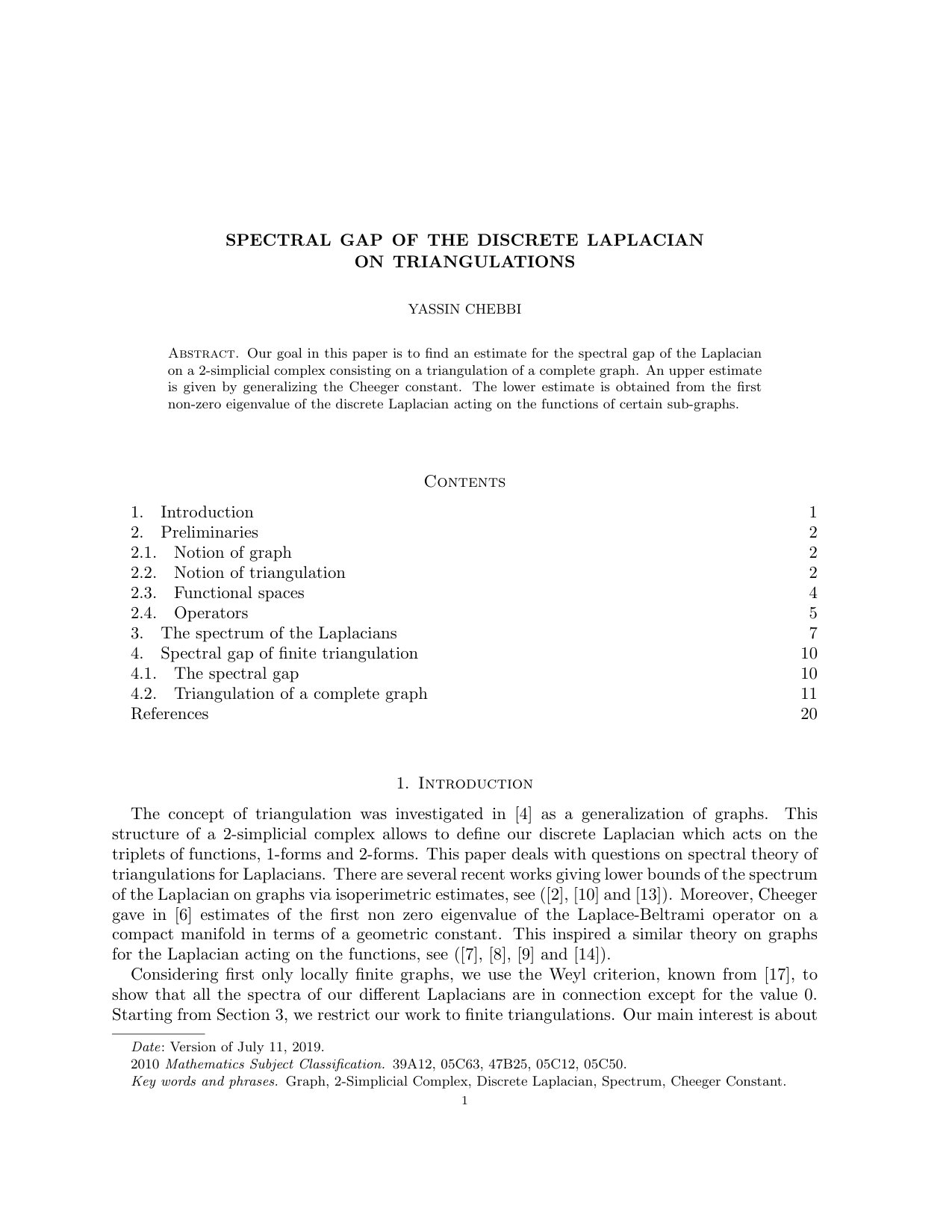 Figure 1
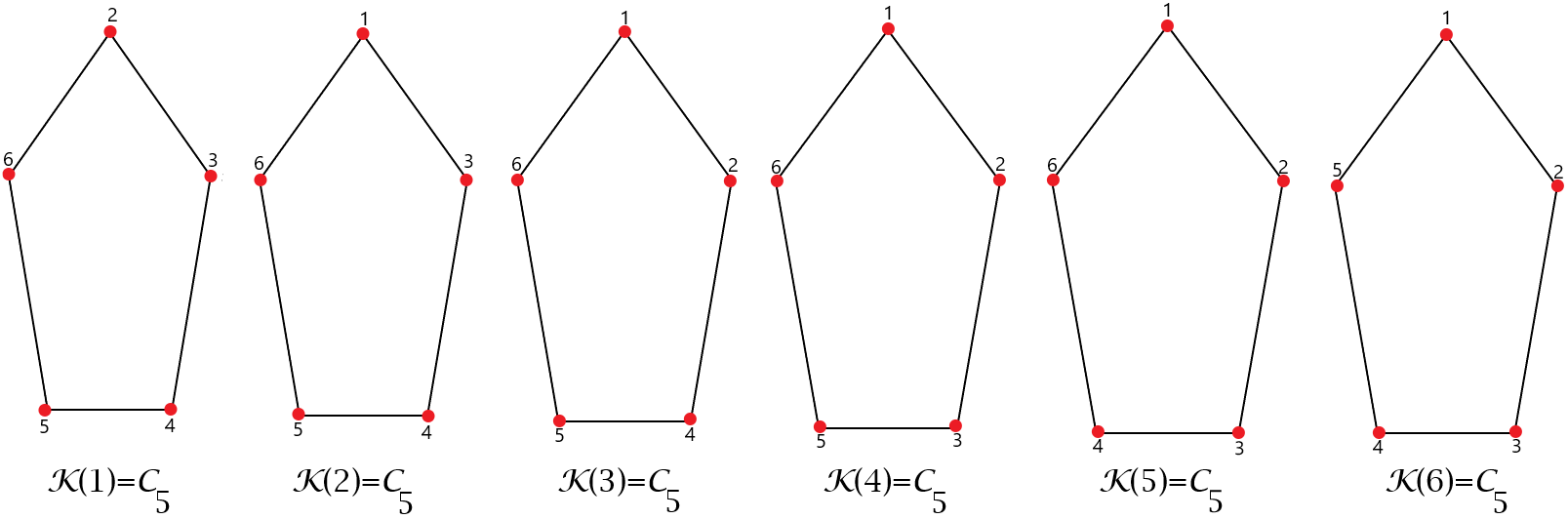 Figure 2
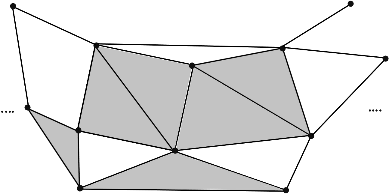 Figure 3
 Figure 4
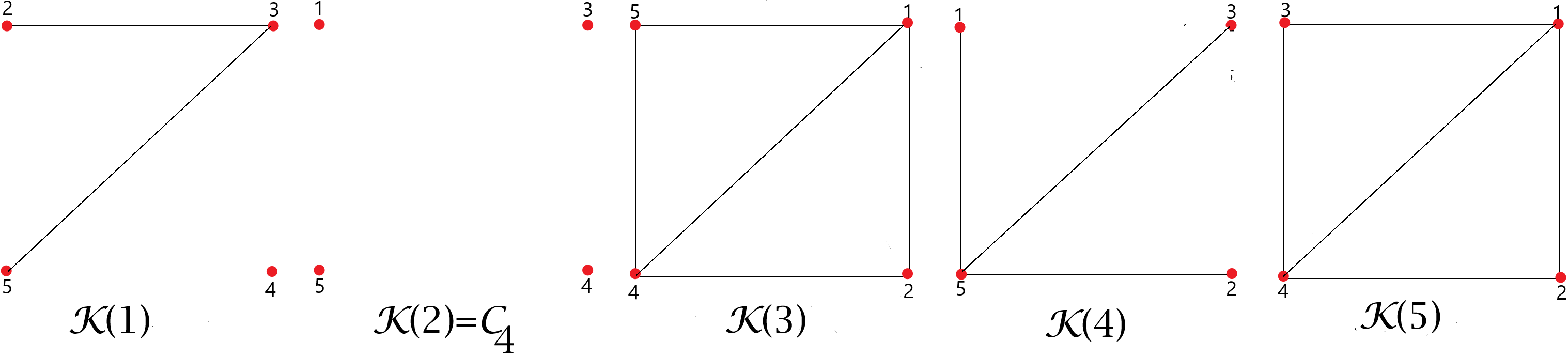 Figure 5
 Figure 6
 Figure 7
 Figure 8
Peer Reviews
No public reviews on file for this paper yet. If you reviewed it on a platform where reviews are public (OpenReview, ICLR, NeurIPS, ICML), you can paste yours below so the community can read it here.
Videos
No videos yet. Explain this paper in a talk, walkthrough, or lecture? Add one.
Spectral Gap of The Discrete Laplacian
on Triangulations
Yassin CHEBBI
Laboratoire de Mathématiques Jean Leray, Faculté des Sciences, CNRS, Université de Nantes, BP 92208, 44322 Nantes, France
Université de Monastir, LR/18ES15, Tunisie
[email protected], [email protected]
(Date: Version of March 12, 2024)
Spectral Gap of The Discrete Laplacian
on triangulations
Yassin CHEBBI
Laboratoire de Mathématiques Jean Leray, Faculté des Sciences, CNRS, Université de Nantes, BP 92208, 44322 Nantes, France
Université de Monastir, LR/18ES15, Tunisie
[email protected], [email protected]
(Date: Version of March 12, 2024)
Abstract.
Our goal in this paper is to find an estimate for the spectral gap of the Laplacian on a 2-simplicial complex consisting on a triangulation of a complete graph. An upper estimate is given by generalizing the Cheeger constant. The lower estimate is obtained from the first non-zero eigenvalue of the discrete Laplacian acting on the functions of certain sub-graphs.
Key words and phrases:
Graph, 2-Simplicial Complex, Discrete Laplacian, Spectrum, Cheeger Constant.
2010 Mathematics Subject Classification:
39A12, 05C63, 47B25, 05C12, 05C50
Contents
1. Introduction
The concept of triangulation was investigated in [4] as a generalization of graphs. This structure of a 2-simplicial complex allows to define our discrete Laplacian which acts on the triplets of functions, 1-forms and 2-forms. This paper deals with questions on spectral theory of triangulations for Laplacians. There are several recent works giving lower bounds of the spectrum of the Laplacian on graphs via isoperimetric estimates, see ([2], [10] and [13]). Moreover, Cheeger gave in [6] estimates of the first non zero eigenvalue of the Laplace-Beltrami operator on a compact manifold in terms of a geometric constant. This inspired a similar theory on graphs for the Laplacian acting on the functions, see ([7], [8], [9] and [14]).
Considering first only locally finite graphs, we use the Weyl criterion, known from [17], to show that all the spectra of our different Laplacians are in connection except for the value Starting from Section 3, we restrict our work to finite triangulations. Our main interest is about the minimal eigenvalue of the upper Laplacian on 1-forms, to be called the spectral gap. Since there are trivial [math]-eigenvalues, if is the number of vertices and we define the spectral gap to coincide with the -eigenvalue of More precisely, we discuss lower and upper estimates for the spectral gap. It is an open question on the Riemannian manifold case. An upper estimate is given by generalizing Cheeger’s approach for triangulations of a complete graph The Cheeger constant is defined as follows, see [5] and [16]:
[TABLE]
where are nonempty sets, making a partition of and denotes the set of the triangle faces with one vertex in each
Moreover, we obtain a lower bound in terms of the first non-zero eigenvalue of the discrete Laplacian defined on the space of functions on the vertices of certain sub-graphs.
2. Preliminaries
2.1. Notion of graph
Let be a countable set of vertices and a subset of the set of oriented edges. The pair () is called a graph. We assume that is symmetric, ie. When two vertices and are connected by an edge , we say they are neighbors. We denote and The set of neighbors of is denoted by The graph is said locally finite if each vertex belongs to a finite number of edges. The degree or valence of a vertex is the cardinal of the set denoted by If the graph has a finite set of vertices, it is called a finite graph. An oriented graph is given by a partition of
[TABLE]
[TABLE]
In this case for we define the origin the ending and the opposite edge A path is a finite sequence of edges such that if then for all The graph is said connected if any two vertices and can be connected by a path with A cycle is a path whose origin and end are identical, i.e An n-cycle is a cycle with vertices. If no cycles appear more than once in a path, the path is called a simple path. All the graphs we shall consider on the sequel will be:
connected, oriented, without loops and locally finite.
2.2. Notion of triangulation
A triangulation generalize the notion of a graph. This structure gives a general framework for Laplacians defined in terms of the combinatorial structure of a simplicial complex. We refer to ([5],[12]) for more detail.
The set of direct permutations of is denoted by
[TABLE]
Let be the set of all simple 3-cycles. We denote the set of triangular faces which is a subset of quotiented by direct permutations as follows:
[TABLE]
where if is a direct permutation of
Definition 2.1**.**
A triangulation is the triplet where is the set of vertices, is the set of edges and is the set of triangular faces. This structure is denoted also by the pair where is a connected locally finite graph. Indeed, one can have simple 3-cycles that are not oriented faces. A triangulation is said complete, if all the triangles are faces.
Remark 2.2**.**
In this paper, the triangulations are considered as two-dimensional simplicial complexes where all faces are triangles.
Choosing an orientation of a triangulation consists of defining a partition of
[TABLE]
[TABLE]
For each face we denote the opposite face
[TABLE]
Let be a triangulation. We say that is a triangulation of bounded degree, if the exist a non-negative such that for all we have For an edge , we also denote the oriented face by and denote the set of neighbors of the edge
[TABLE]
To define weighted triangulations we need weights, let us give
- •
the weight on the vertices.
- •
the even weight on the oriented edges, i.e
- •
the even weight on oriented faces, ie.
The weighted triangulation is given by the triangulation A triangulation is called homogeneous, if the weights of the vertices, the edges and faces equal As our graph is locally finite, we can define a weight on by
[TABLE]
This weight on any vertex is well defined. A graph is called a normalized graph if for all
2.3. Functional spaces
We denote the set of 0-cochains or functions on by:
[TABLE]
and the set of functions of finite support by Similarly, we denote the set of 1-cochains or 1-forms on by:
[TABLE]
and the set of 1-forms of finite support by Moreover, we denote the set of 2-cochains or 2-forms on by:
[TABLE]
and the set of 2-forms of finite support by
We consider on the weighted triangulation the following Hilbert spaces, let us give
- •
The Hilbert space of functions:
[TABLE]
with the inner product
[TABLE]
- •
The Hilbert space of 1-forms:
[TABLE]
with the inner product
[TABLE]
- •
The Hilbert space of 2-forms:
[TABLE]
with the inner product
[TABLE]
The direct sum of the spaces , and can be considered as a Hilbert space denoted by , that is
[TABLE]
endowed with the inner product
[TABLE]
2.4. Operators
In this section, we recall the concept of difference and exterior derivative operators introduced on weighted triangulations. We refer to [3] and [5] for more details. This permits to define the discrete Laplacians acting on functions, 1-forms and 2-forms.
2.4.1. The difference operator
It is the operator given by
[TABLE]
2.4.2. The co-boundary operator
It is the formal adjoint of denoted by
[TABLE]
acts as
[TABLE]
and satisfies
[TABLE]
2.4.3. The exterior derivative
It is the operator given by
[TABLE]
2.4.4. The co-exterior derivative
It is the formal adjoint of denoted by
[TABLE]
acts as
[TABLE]
and satisfies
[TABLE]
2.4.5. The discrete Laplacian
In this section, we will always consider a weighted triangulation The discrete Laplacian acting on functions is given by
[TABLE]
for all and The discrete Laplacian acting on 1-forms is given by
[TABLE]
for all and The discrete Laplacian acting on 2-forms is given by
[TABLE]
for all and To define the Gauß-Bonnet operator, let us begin by defining the operator
[TABLE]
by
[TABLE]
and the formal adjoint of is given by
[TABLE]
The Gauß-Bonnet operator is defined on into itself by:
This operator is of Dirac type and is motived by the Hodge Laplacian:
[TABLE]
Remark 2.3**.**
The operator is called the full Laplacian and defined as where (resp. ) is called the lower Laplacian (resp. the upper Laplacian).
3. The spectrum of the Laplacians
In this section, we will prove the relation between the spectrum of and that of The following results due to the Weyl’s criterion known from [17] to characterize the spectrum of our operators.
Weyl’s criterion: Let be a separable Hilbert space, and let be a bounded self-adjoint operator on Then is in the spectrum of if and only if, there exists a sequence so that and
We denote the spectrum of We refer here to [1], which proves that in a normalized graph.
Proposition 3.1**.**
Let be a homogeneous triangulation of bounded degree. Then, we have
[TABLE]
*Proof: *
At first, we notice that the hypothesis assures that all operators are bounded. Through the Weyl’s criterion, set in the spectrum of then there is a sequence in such that:
[TABLE]
So, we should find a sequence in such that
[TABLE]
Set
[TABLE]
First, let us show that We have that
[TABLE]
Thus the term tends to as Therefore, there exist and such that for all we have It remains to show that In fact, we have:
[TABLE]
Since the operator is bounded. Hence, there exists a constant such that and we have that:
[TABLE]
Using the same method as the first step, set the non-zero constant Then there exists a sequence in such that We consider a sequence in define as follows:
[TABLE]
Proposition 3.2**.**
Let be a finite weighted triangulation. Then, we have
[TABLE]
*Proof: *
Let we consider Thus, we have
[TABLE]
Moreover, we have
[TABLE]
By Rayleigh principle, we obtain that
[TABLE]
Proposition 3.3**.**
Let be a homogeneous finite triangulation. Then, we have
[TABLE]
*Proof: *
Let we consider Then, we have
[TABLE]
Using for all We have
[TABLE]
On other hand, we have
[TABLE]
From Rayleigh principle, we obtain:
[TABLE]
4. Spectral gap of finite triangulation
4.1. The spectral gap
We describe the discrete Hodge theory due to Eckmann [11]. This is a discrete analogue of Hodge theory in Riemannian geometry. Furthermore, it applies to any finite simplicial complex, and not only to manifolds. Let us begin with
Lemma 4.1**.**
We have that
[TABLE]
*Proof: *
It is clear that On the other hand, if for all we have that
[TABLE]
Then, As the previous reasoning, we prove that and After, if then
[TABLE]
which shows that
Since we have the discrete Hodge decomposition
[TABLE]
In particular, it follows that the space of harmonic forms can be identified with the homology of
[TABLE]
The same holds for the homology of giving
[TABLE]
For a triangulation, the space is always in the kernel of the upper Laplacian, and considered to be its trivial zeros. There can be more zeros in the spectrum, since As this leads to the following definition:
Definition 4.2**.**
(The spectral gap)* The spectral gap of a finite triangulation denoted is the minimal eigenvalue of the upper Laplacian on 1-forms:*
[TABLE]
the equality follows from
Remark 4.3**.**
Generally, the spectral gap is the difference between [math] and the first non-zero eigenvalue, see ([7], [8] and [9]). This definition coincides with the definition 4.2 in the case where the eigenvalue is not zero ( i.e there is no harmonic 1-form).
The following proposition gives a characterization of the spectral gap.
Proposition 4.4**.**
The spectrum of the Laplacian is composed of reals eigenvalues ranked in ascending order:
[TABLE]
Moerever, we have that
[TABLE]
*Proof: *
Since the dimension of the space is the number of the trivial zeros of the upper Laplacian. Using the rank theorem for the operator we get that
[TABLE]
Proposition 4.5**.**
Let be a finite triangulation. Then, we have
[TABLE]
*Proof: *
Applying the Rank theorem for we obtain
[TABLE]
And since then
[TABLE]
Remark 4.6**.**
In the case where we have and
Example 4.7**.**
Consider the triangulation such that all the triangles are faces as in Figure Using the Rank theorem, we have:
[TABLE]
Then,
4.2. Triangulation of a complete graph
The aim of this part is to provide effective estimates for the spectral gap of a triangulation of a complete graph. Let us begin by
Definition 4.8**.**
A triangulation of a complete graph is the pair where is the complete graph of vertices and is the set of triangular faces.
First, we give a result assuring that our spectral gap is zero in a triangulation of a complete graph. This result is a consequence of Proposition 4.5.
Corollary 4.9**.**
Let be a homogeneous triangulation of a complete graph. Then, we have
[TABLE]
4.2.1. Upper estimates of the spectral gap
We would like to find a concrete upper estimate of the spectral gap in relation with the number of oriented faces in a simple triangulation of a complete graph.
Proposition 4.10**.**
Let be a homogeneous triangulation of a complete graph. Then, we have
- i)
** 2. ii)
If is a simple complete triangulation then
Lemma 4.11**.**
Let be a finite triangulation. Then
[TABLE]
*Proof of Lemma 4.11: *
It is clear that Let there is such that Since then where Hence
[TABLE]
*Proof of Proposition 4.10: *
- i)
Let then it exists such that We calculate
[TABLE]
Hence By Lemma 4.11, we have that 2. ii)
Let if is complete, then we have
[TABLE]
By Lemma 4.11, we get that
Remark 4.12**.**
The value [math] is not always in the spectrum of the full Laplacian It depends on the value of due to the fact that In particular, if is a complete triangulation we have that
Corollary 4.13**.**
Let be a homogeneous triangulation of a complete graph. Then, we have
[TABLE]
Moreover, is the complete triangulation if and only if
*Proof: *
From Proposition 4.10 and Lemma 4.11, we deduce that Moreover, The Proposition 3.2 give an upper estimate of the lower spectrum of
[TABLE]
If then Then, the inegality (4.1) give an upper estimate of the lower spectrum acting as:
[TABLE]
If alors and Then the triangulation is complete. By Proposition 4.10,
Remark 4.14**.**
In a homogeneous triangulation of a complete graph, we have always:
[TABLE]
Our goal now is to find the best estimate of the eigenvalue when is large enough. Given a homogeneous triangulation of a complete graph, the Cheeger constant is defined as follows, see ([5], [16]):
[TABLE]
where are nonempty sets, considered as a partition of and denotes the set of the oriented faces with one vertex in each It is clear that:
[TABLE]
Let are two finite sets such that we define the set:
[TABLE]
Theorem 4.15**.**
If holds, then the spectral gap satisfies the following upper estimate
[TABLE]
*Proof: *
Set and be a partition of which realizes the minimum in We define by
[TABLE]
where is a map such that It is clear that Therefore, we have
[TABLE]
and
[TABLE]
By the Rayleigh’s principle, we have:
[TABLE]
Example 4.16**.**
We consider the triangulation with and \mathcal{F}=\{({\color[rgb]{1,0,0}1},2,3),({\color[rgb]{1,0,0}1},2,4),({\color[rgb]{1,0,0}1},3,4)\}. Then, we have Applying Theorem 4.15, we obtain that
[TABLE]
Example 4.17**.**
We consider the triangulation with and \mathcal{F}=\{({\color[rgb]{1,0,0}1},2,3),({\color[rgb]{1,0,0}1},2,4),({\color[rgb]{1,0,0}1},3,4),({\color[rgb]{1,0,0}1},2,5),({\color[rgb]{1,0,0}1},3,5),({\color[rgb]{1,0,0}1},4,5)\}. Then, we have Applying Theorem 4.15, we obtain that
[TABLE]
4.2.2. Lower estimates of spectral gap
First, we recall some lower estimates of the spectral gap of on connected graphs, see ([9],[14]). Our objective is to find a lower estimate of the spectral gap from the second eigenvalue of
Let be a finite triangulation and We define the set of edges :
[TABLE]
Denote by the associated graph of the vertex where:
[TABLE]
Remark 4.18**.**
In a triangulation of a complete graph, the hypothesis (4.2) assures that, for all And then, we have that for all
Theorem 4.19**.**
Let be a homogeneous triangulation of a complete graph. Assume that, for all then
[TABLE]
*Proof: *
Given an eigenfunction associated of such that Then, we have
[TABLE]
For each vertex we can define on the function Then, we have for all Next, we have
[TABLE]
Thus,
[TABLE]
Since is the set oriented edges, we have
[TABLE]
Then On other hand, we have
[TABLE]
Applying the Min-Max principle, we obtain that
[TABLE]
Remark 4.20**.**
This theorem is interesting in the case of triangulations of a complete graph where its sub-graphs are connected in such a way that we have To ensure this assumption, we should take triangulations with a large number of triangular faces.
The next result is obtained from the lower estimate of the spectral gap of the discrete Laplacian see [8] and [9].
Corollary 4.21**.**
Let be a homogeneous triangulation of a complete graph. Assume that for all then
[TABLE]
with for all
*Proof: *
Let an eigenfunction of such that Using Theorem 4.19, we obtain that
[TABLE]
Example 4.22**.**
We consider the triangulation with and Using Theorem 4.19, we obtain that:
[TABLE]
Example 4.23**.**
We consider the triangulation with and Using Theorem 4.19, we obtain that:
[TABLE]
The spectral gap of a discrete graph is a monotonously increasing function of the set of edges. In other words, adding an edge always increases of the second eigenvalue or keeps it unchanged, provided that we have the same set of vertices, see [15].
Proposition 4.24**.**
Let be a connected graph and let be a graph obtained from by adding one edge between two vertices. Then the following hold:
[TABLE]
Example 4.25**.**
We consider the triangulation with and Using Proposition 4.24, we obtain that By Theorem 4.19, we have:
[TABLE]
Acknowledgments**:** I would like to sincerely thank my PhD advisors, Professors Colette Anné and Nabila Torki-Hamza for helpful discussions. I am very thankful to them for all the encouragement, advice and inspiration. I would also like to thank the Laboratory of Mathematics Jean Leray and the research unity (UR/13 ES 47) for their continuous support. This work was partially financially supported by the ”PHC Utique” program of the French Ministry of Foreign Affairs and Ministry of higher education and research and the Tunisian Ministry of higher education and scientific research in the CMCU project number 13G1501 ”Graphes, Géométrie et Théorie Spectrale”.
The reference list from the paper itself. Each links out to its DOI / PubMed record.
- 1[1] H. Ayadi: Spectra of Laplacians on an infinite graph , Oper. Matrices, 11, no.2, 567-586, 2017.
- 2[2] N. Alon and V.D. Milman: λ 1 , subscript 𝜆 1 \lambda_{1}, isoperimetric inequalities for graphs, and superconcentrators , J. Combin. Theory Ser. B, 38, no. 1, 73-88, 1985.
- 3[3] C. Anné and N. Torki-Hamza: The Gauß-Bonnet operator of an infinite graph , Anal. Math. Phys. 5, no.2, 137-159, 2015.
- 4[4] Y. Chebbi: The discrete Laplacian of a 2-simplicial complex , Potential Analysis, 49, no.2, 331-358, 2018.
- 5[5] Y. Chebbi: Laplacien discret d’un 2-complexe simplicial , HAL Id: tel-01800569, 2018.
- 6[6] J. Cheeger: A lower bound for the smallest eigenvalue of the Laplacian , Problems in Analysis (Papers dedicated to Salamon Bochner, 1969), pp. 195-199, Princeton University Press, Princeton, NJ, 1970.
- 7[7] F.R.K Chung: Spectral graph theory , CBMS Regional Conference Series in Mathematics. 92. Providence, RI: American Mathematical Society (AMS). xi, p. 207, 1994.
- 8[8] F. Chung, A. Grigoryan, S-T. Yau: Higher eigenvalues and isoperimetric inequalities on Riemannian manifolds and graphs , Comm. Anal. Geom., 8, no. 5, 969-1026, 2000.