Eigenvalues of the non-backtracking operator detached from the bulk
Simon Coste, Yizhe Zhu

TL;DR
This paper analyzes the non-backtracking spectrum of stochastic block models in a dense regime, identifying a key eigenvalue inside the bulk and introducing a new perturbation theorem for quadratic eigenvalue problems.
Contribution
It provides a detailed spectral analysis of the non-backtracking operator in dense stochastic block models and introduces a novel Bauer-Fike variant for quadratic eigenvalue problems.
Findings
Existence of a real eigenvalue inside the bulk near a specific location.
Characterization of the non-backtracking spectrum in dense regimes.
Introduction of a new Bauer-Fike theorem variant for quadratic eigenvalue problems.
Abstract
We describe the non-backtracking spectrum of a stochastic block model with connection probabilities . In this regime we answer a question posed in Dall'Amico and al. (2019) regarding the existence of a real eigenvalue `inside' the bulk, close to the location . We also introduce a variant of the Bauer-Fike theorem well suited for perturbations of quadratic eigenvalue problems, and which could be of independent interest.
Click any figure to enlarge with its caption.
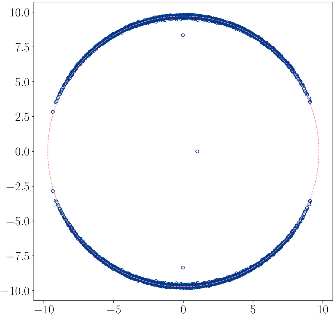 Figure 1
 Figure 2
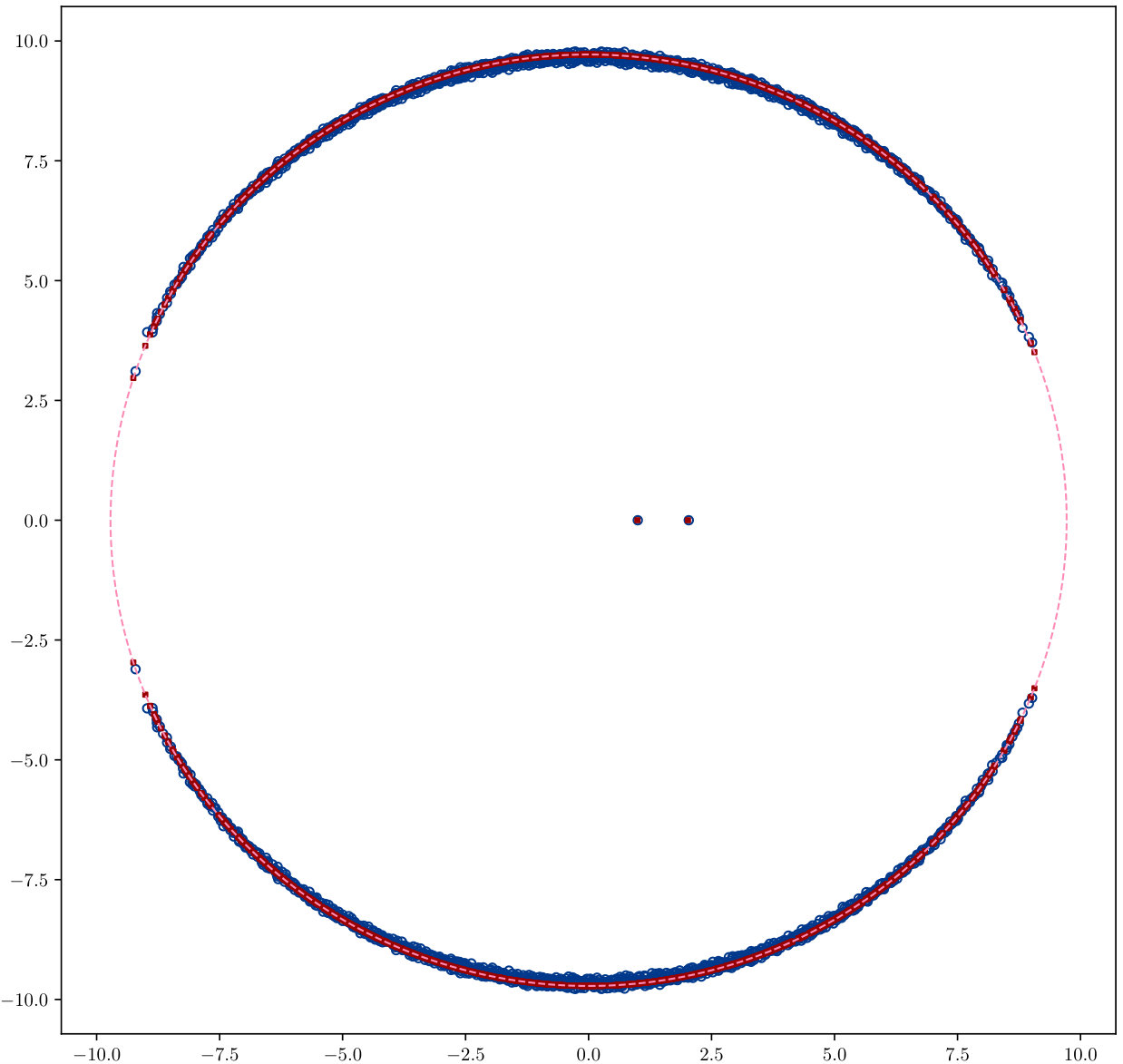 Figure 3
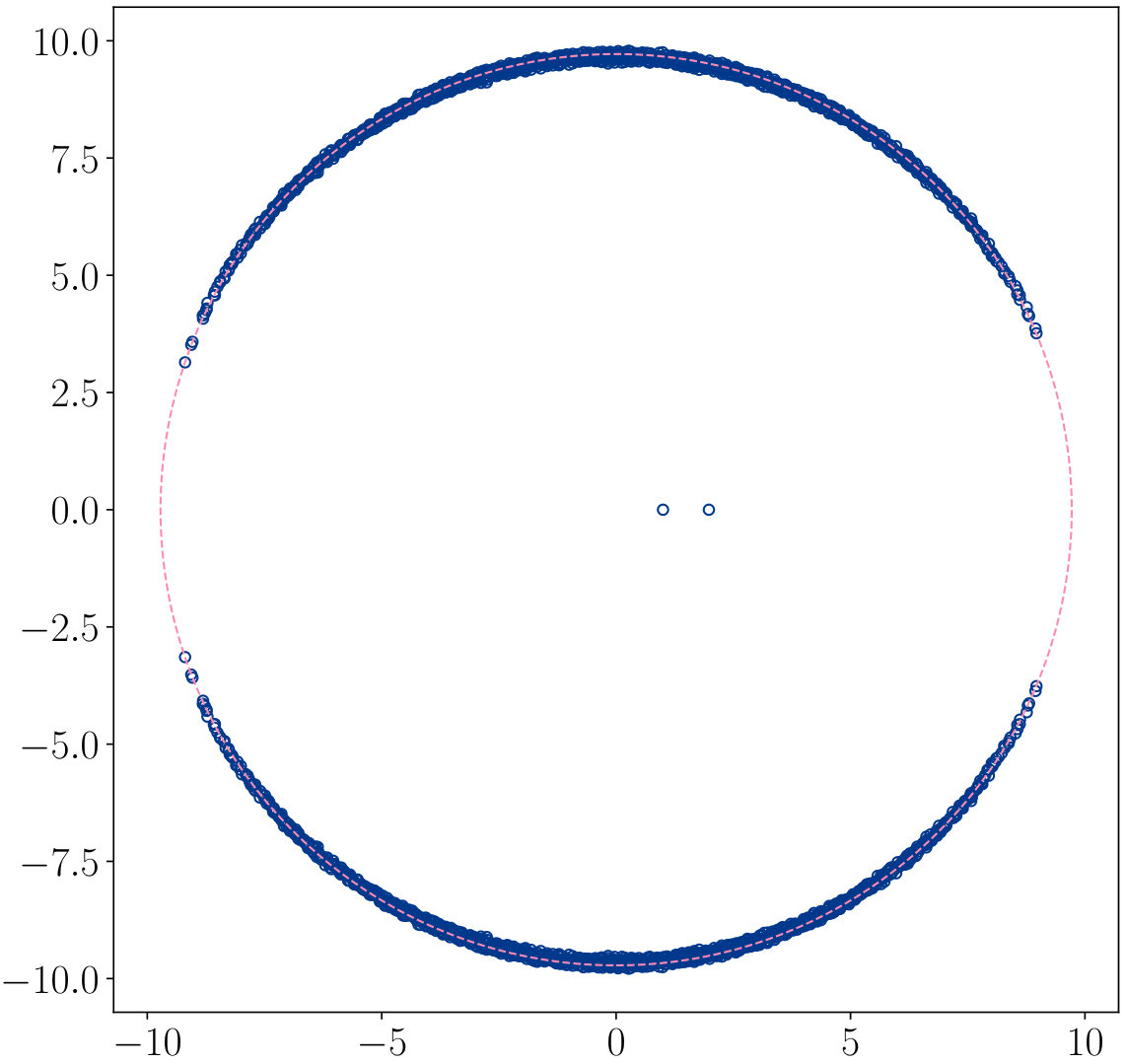 Figure 4
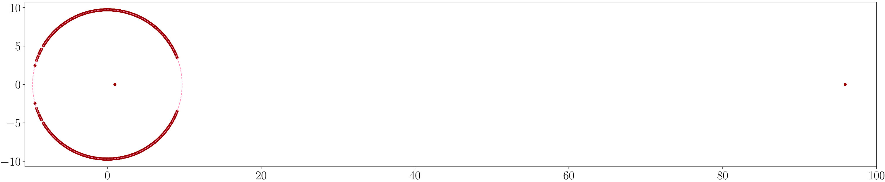 Figure 5
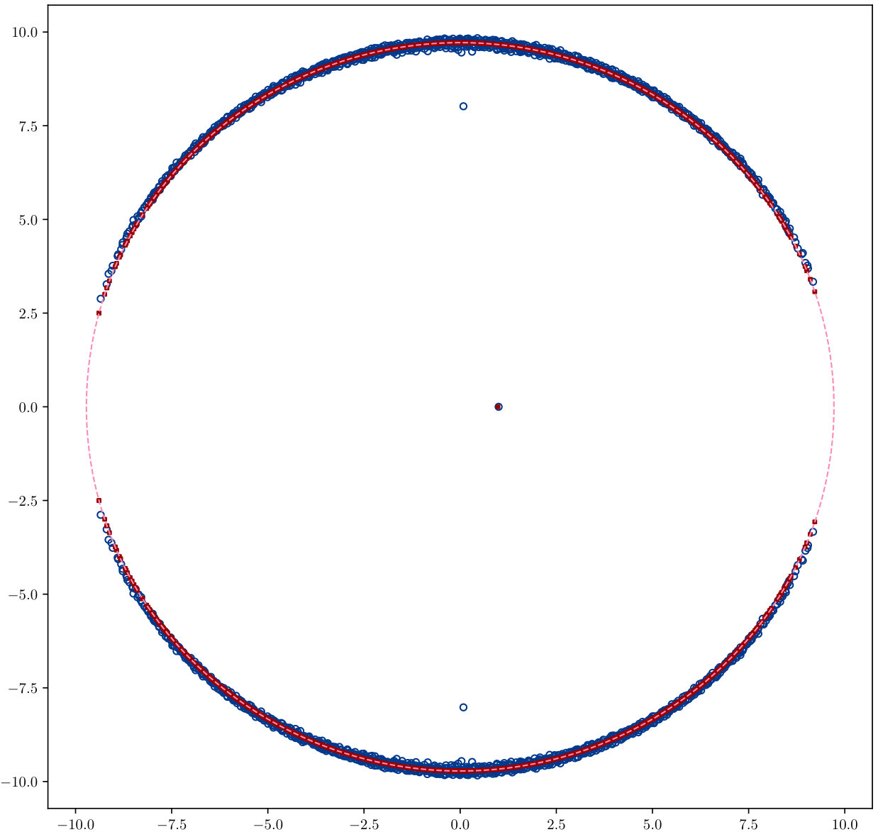 Figure 6
Peer Reviews
No public reviews on file for this paper yet. If you reviewed it on a platform where reviews are public (OpenReview, ICLR, NeurIPS, ICML), you can paste yours below so the community can read it here.
Videos
No videos yet. Explain this paper in a talk, walkthrough, or lecture? Add one.
Eigenvalues of the non-backtracking operator detached from the bulk
Simon Coste
INRIA Paris, DYOGENE team
Office C330
and
Yizhe Zhu
Department of Mathematics, University of California, San Diego, La Jolla, CA 92093
Abstract.
We describe the non-backtracking spectrum of a stochastic block model with connection probabilities . In this regime we answer a question posed in [15] regarding the existence of a real eigenvalue ‘inside’ the bulk, close to the location . We also introduce a variant of the Bauer-Fike theorem well suited for perturbations of quadratic eigenvalue problems, and which could be of independent interest.
Key words and phrases:
non-backtracking operator, stochastic block model, non-Hermitian perturbation, quadratic eigenvalue problem
Y.Z. is partially supported by NSF DMS-1712630.
1. Introduction
For any real matrix with size , its non-backtracking operator is the real matrix indexed by the coordinates of the non-zero entries of , and is defined by
[TABLE]
The non-backtracking matrix of a graph is the non-backtracking matrix of its adjacency matrix, and it is closely related to the Zeta function of the graph [29]. Its spectrum was first studied in the case of finite graphs and their universal covers [19, 7, 27, 20, 29, 5]. Recently, the non-backtracking operator attracted a lot of attention from random graph theory as a very powerful tool. In the spectral theory of random graphs, it was a key element in a new proof of the Alon-Friedman theorem for random regular graphs [11]. In the same vein it has been used later to study the eigenvalues of random regular hypergraphs [16], random bipartite biregular graphs [13] and homogeneous or inhomogeneous Erdős-Rényi graphs [21, 31, 12, 18, 8, 3, 9]. Very recently, the real eigenvalues were used to prove estimates on the vector-colouring number of a graph [6].
Most of the results focus on the eigenvalues of large magnitude, those which lie outside the bulk of the spectrum. They are known to be the ‘most informative’ eigenvalues, as they capture some essential features about the structure of the graph. For instance, in community detection, the appearance of certain outliers indicates when the community structure can be recovered [12, 21]. A cornerstone result was that even in the difficult dilute case, where the connection probabilities are of order , reconstruction was feasible (under some condition) by looking at the eigenvalues of the non-backtracking matrix appearing outside the ‘bulk’ of eigenvalues.
It was recently observed in [15, Section 3.2] that in fact, there is a real eigenvalue isolated inside the bulk that corresponds to the ratio of the two largest eigenvalues outside the bulk, as displayed in the right panel of Figure 1. Recall that is non-Hermitian with a complex spectrum, so that ‘inside’ the bulk is understood as eigenvalues inside the circle of the spectrum. To the best of our knowledge, this phenomenon has not been rigorously studied yet. In this paper, we prove the existence of this real eigenvalue inside the bulk for the stochastic block model (SBM) in the regime where the mean degree goes to infinity faster than .
Notations
Throughout the paper, we will adopt the conventional notations when , when and when is bounded. All the results depend on the parameter , the size of the graph, which is seen as large through . For any matrix , we denote the spectral norm of as .
1.1. Setting: the SBM in the logarithmic regime
Consider a stochastic block model with an even number of vertices, two blocks of equal size , and two probability parameters : if are vertices in the same block then they are connected with probability , and if they are in different blocks they are connected with probability . We will place ourselves under the regime
[TABLE]
for some constants . The last condition is technical: we will see that it is here to ensure that two separated outliers appear in the spectrum of the adjacency matrix, and are of the same order. This assumption is crucial in our perturbation analysis, see Remark 4.2 for further discussion.
It is known (see for example [10, Chapter 3]) that when , the graph (the Erdős-Rényi model) is ‘almost regular’ in the sense that all degrees are concentrated around . In general, it can be shown that when then is almost regular with degrees concentrated around
[TABLE]
See Subsection 3.4 for a proof. For this reason, we will denote by the mean degree and by the mean difference degree:
[TABLE]
where is the number of neighbors of vertex , and (resp. ) is the number of neighbors of vertex which do not have the same type as (resp. which have the same type as ). Under assumption (A), can be either positive or negative, and are of the same order.
Our assumptions (A) imply that the mean degree is and the mean difference degree has the same order as . Finally, the adjacency matrix of the graph is the matrix defined by , where denotes the event that and are connected.
1.2. Main results
Let be any finite graph with adjacency matrix . The Ihara-Bass formula gives a connection between the spectrum of defined in (1.1) and a quadratic eigenvalue problem: for any complex ,
[TABLE]
see [7, 20, 27]. The zeros of the polynomial are usually called, with an abuse of language, the non-backtracking spectrum of , the two additional eigenvalues appearing with multiplicity in (1.2) being usually called trivial. The non-backtracking spectrum can be expressed as the eigenvalues of a smaller matrix :
[TABLE]
where is the diagonal degree matrix. This representation of the spectrum of in terms of is extremely useful: to compute the spectrum of , we do not have to construct the matrix , and we can analyze the spectrum of directly from .
Using these facts, we answer the question posed in [15] regarding the existence of an isolated eigenvalue inside the bulk, at least under the assumptions (A). We also give a detailed description of the non-backtracking spectrum that is similar to the one given in [31] for Erdős-Rényi graphs.
Theorem 1.1**.**
Let be the non-backtracking operator of a stochastic block model satisfying assumption (A). We order the eigenvalues of by decreasing modulus: .
With probability , the spectrum of can be described as follows. First, the smallest eigenvalues in modulus are the trivial eigenvalues and , each with multiplicity .
Then, in the non-trivial eigenvalues , there are four real eigenvalues which are isolated, two ‘outliers’
[TABLE]
and two ‘insiders’
[TABLE]
All the other eigenvalues with are located within distance of a circle of radius . Moreover, the real parts of eigenvalues of are asymptotically distributed as the semi-circle distribution supported on .
To present our approach in the most efficient and clear way, we state and prove the theorem in the simplest regime, when there are only two blocks and when the community structure appears in the spectrum through the presence of an extra outlier near . It is straightforward to check that our proof can be extended to a diversity of settings, when the mean degree is . We state this as an informal result:
Assume that with high probability the degree of each vertex is and the spectrum of the adjacency matrix has outliers far outside , say , and . Assume are are of the same order. Then with high probability its non-backtracking spectrum will have eigenvalues near for , then eigenvalues near , and all the other eigenvalues will be located within distance of the circle of radius .
Remark 1.2*.*
The concentration results we have in Section 3 work for general inhomogeneous random graphs with outliers of the same order. Our modified Bauer-Fike theorem given in Theorem 2.2 works for general inhomogeneous random graphs as well, as long as each vertex has almost regular degree . Therefore all the analysis in Section 4 can be extended to the case we mentioned above for outliers.
The presence of bulk insiders in Theorem 1.1 and in the preceding statement are illustrated in Figure 1 for a realization of an Erdős-Rényi graph and a realization of an SBM graph. Note that the description of the spectrum of in the preceding theorem is much more precise than Theorem 1.5 in [31]. This comes from the fact that their perturbation parameter goes to infinity (see Theorem 1.5 in [31] for the exact statement, where the scaling parameter is different from ours). Our method includes a tailored version of the Bauer-Fike theorem suited for perturbations of matrices like (1.3), which yields perturbation bounds that are better than the classical Bauer-Fike theorem in terms of the order of magnitude, and without which the existence of the two eigenvalues at and near would not follow. We think such variants of the Bauer-Fike theorem could be of independent interest.
1.3. Bulk insiders and community detection
The real eigenvalue of inside the bulk is closely related to community detection problems for SBMs. An interesting heuristic spectral algorithm based on the Bethe Hessian matrix was proposed in [32, 26]. The Bethe Hessian matrix, sometimes called deformed Laplacian ([17, 15]), is defined as
[TABLE]
where is a regularizer to be carefully tuned. It is conjectured in [26] that a spectral algorithm based on the eigenvectors associated with the negative eigenvalues of with is able to reach the information-theoretic threshold confirmed in [23, 12, 25, 24] for community detection in the dilute regime. In a subsequent work [15], the authors crafted a spectral algorithm based on with and empirically showed it outperforms already known spectral algorithms. Their choice of was motivated by the conjectured value of the real eigenvalue inside the bulk. The gain in using instead of in spectral algorithms mainly comes from the fact that has a smaller dimension than , is Hermitian, and is easiest to build from — nearly no preprocessing is needed, in contrast with non-backtracking matrices [12, 21], self-avoiding path matrices [23] or graph powering matrices [1].
The relation between the Bethe Hessian matrix and the non-backtracking operator is given by the Ihara-Bass formula (see (1.2) above). Therefore, a good understanding of the real eigenvalues of the non-backtracking operator is the first step towards understanding the theoretical guarantee of the heuristic algorithms purposed in [26, 15].
Unfortunately, our proof techniques do not work in the dilute regime. In the regime studied in this paper, community detection problems are now very well understood and clustering based on the second eigenvector of has been proven to yield exact reconstruction (see [2]). Our result should instead be seen as a preliminary step in view of
- proving the existence of bulk insiders in the dilute regime, 2) showing their usefulness in practical reconstruction. It will be helpful in practice to have a better understanding of the eigenvectors for the Bethe Hessian matrix, and we leave it as a future direction.
The key obstacle is the lack of concentration of degrees profiles, which tells us random graphs with bounded expected degrees are far away from being ‘roughly’ regular (see also the discussion in Subsection 3.4). Without this property, our perturbation analysis does not apply.
Organization of the paper
In Section 2, we first state some classical facts on the non-backtracking spectrum of graphs then we state and prove a perturbation theorem which is well suited for quadratic eigenvalue problems and improves the classical Bauer-Fike results. In Section 3, we gather several facts on stochastic block models. Then we study the spectrum of as in (1.3) and a suitably chosen perturbation of (defined later in (3.2)). In Section 4 we prove the main theorem.
2. Perturbation of the non-backtracking spectrum
2.1. The non-backtracking spectrum
When the graph is regular with degree , the diagonal matrix satisfies , and we can relate the eigenvalues of with the eigenvalues of through exact algebraic relations as in the following elementary lemma.
Lemma 2.1**.**
Let be a Hermitian matrix with eigenvalues and let be a nonzero complex number. Then, the characteristic polynomial of the matrix
[TABLE]
is given by , and the eigenvalues of are the complex numbers (counted with multiplicities) which are solutions of for .
Similar exact relations have also been used when the graph has a very specific structure, like bipartite biregular (see [13]). When the graph does not exhibit such a simple structure, the relation between and becomes more involved. Several Ihara-Bass-like formulas are available (see for instance [32, 8, 4]), but they are usually hard to analyze.
As cleverly noted in [31], the spectrum of as in (1.3) is hard to describe in terms of the spectrum of , but the spectrum of in the preceding lemma is completely explicit in terms of the spectrum of , even if has no specific structure. It is therefore quite natural to study the spectrum of using the spectrum of , then use perturbation theorems to infer results on the ‘true’ non-backtracking spectrum, the spectrum of . This is done in [31] through a combination of the Bauer-Fike theorem and a refinement of the Tao-Vu replacement principle [28].
The celebrated Bauer-Fike theorem says that* if a square matrix is diagonalizable, say for a diagonal matrix and a non-singular matrix , then under a perturbation , every eigenvalue of the matrix is within distance of an eigenvalue of *, where , and is the condition number (see for instance [12]).
We observe that the Bauer-Fike theorem, while optimal in the worst case, is indeed extremely wasteful when applied to and . Taking into account the specific structure of and yields a better perturbation bound at virtually no cost, as shown in the next section.
2.2. Bauer-Fike theorems for quadratic eigenvalue problems
A quadratic eigenvalue problem (QEP) consists of finding the zeroes of the polynomial equation
[TABLE]
where are square matrices, and is non-singular. Such problems appear in a variety of contexts and there exists an extensive literature on them, mainly from a numerical point of view (see the survey [30]).
The triplet can be replaced with by the triplet without changing the problem, so we will be interested in the case where . In this case, one can easily check that the solutions of (2.1) are the eigenvalues of the matrix
[TABLE]
which is called a linearization of the problem. In this section, we will present extensions of the Bauer-Fike theorem for linearizations of quadratic eigenvalue problems.
If both matrices and are diagonal, say and , then it is easily seen through elementary linear algebra operations that
[TABLE]
and the eigenvalues of are the complex solutions of the collection of quadratic equations for .
We say the matrices and are co-diagonalizable if there is a common non-singular matrix such that and are diagonal. If are co-diagonalizable, then the identity (2.2) still holds with being the eigenvalues of and being those of . As a consequence, we say that that is QEP-diagonalizable if and are co-diagonalizable. This is equivalent to ask that the matrix is diagonalizable for any .
Our main tool for the perturbation analysis is the following theorem.
Theorem 2.2**.**
Let be matrices. We define
[TABLE]
Suppose is QEP-diagonalizable, with and being diagonalized by the common matrix . Then, for any eigenvalue of , there is an eigenvalue of such that
[TABLE]
Moreover, ‘multiplicities are preserved’ in the following sense: Denote the RHS of (2.3) and . If are the eigenvalues of and is a subset of such that
[TABLE]
where for , then the number of eigenvalues of in is exactly equal to .
Remark 2.3*.*
Theorem 2.2 is stated for two general matrices and . However, the inequality (2.3) will yield good perturbation bound only when we can control the difference between , the difference between , and the condition number .
Proof.
Assume is an eigenvalue of . The matrix is then singular. Assume, in addition, that is not an eigenvalue of . Then, the matrix is non-singular. We have
[TABLE]
As a consequence the matrix is singular, which directly implies that is an eigenvalue of . therefore by the definition of spectral norm,
[TABLE]
As noted before the statement of the theorem, if is QEP-diagonalizable then the matrix is indeed diagonalizable: if is the diagonal matrix of eigenvalues of , the diagonal matrix of eigenvalues of , and their common diagonalization matrix, then , and the eigenvalues of are the complex numbers , so
[TABLE]
From this, we infer that there is a such that . Let us denote and the two complex solutions of (they are eigenvalues of ), then
[TABLE]
which implies that
[TABLE]
If and were both strictly greater than , the preceding inequality would be violated. One of those distances is thus smaller than , thus proving (2.3).
The ‘multiplicities preserved’ part is then proven as usual with the complex argument principle, see for instance [14, Appendix A]. ∎
When applying the preceding result with , one gets the following corollary.
Corollary 2.4**.**
Let
[TABLE]
where are square matrices and are such that is QEP-diagonalizable with and diagonalized by the common matrix . Then, for any eigenvalue of , there is an eigenvalue of such that
[TABLE]
Remark 2.5* (Comparison with classical Bauer-Fike).*
Casting the classical Bauer-Fike theorem in this setting would yield an error term of , where is the diagonalization matrix of . We thus gain the whole square root, and we do not need to compute the condition number of . This improvement is remarkable when the matrix is itself Hermitian, for in this case is unitary and , thus reducing the error term to . If we had invoked the classical Bauer-Fike theorem instead, the error term would be , which can be far bigger than . In fact, the matrix is not Hermitian in general, and its diagonalization matrix might be either difficult to compute or ill-conditioned: in [31], the bound obtained by the authors is , where is the connection probability for an Erdős-Rényi graph . Our version of the Bauer-Fike theorem shows that for QEP, the only parameters at stake in perturbations are those of the original matrices and , not those of the linearization of the QEP.
3. The stochastic block model in the logarithmic regime
In this section, we collect results from the literature on stochastic block models or inhomogeneous Erdő-Rényi graphs, based on which we prove several quick results for our models, as given in Proposition 3.1, Proposition 3.2 and Corollary 3.3.
3.1. Outliers of the adjacency matrix
The concentration of the spectral norm for the SBMs follows immediately from the spectral norm bounds given in [22, 8] for inhomogeneous random matrices and random graphs. Recall Assumption (A). The following statement can be found for example in Example 4.1 of [22]: assume , then
[TABLE]
Also from Equation (2.4) in [8], there exists a constant such that
[TABLE]
Taking in the inequality above, we have with probability that
[TABLE]
Since all the eigenvalues of are , and under assumption (A), the Weyl eigenvalue inequalities for Hermitian matrices yields the following proposition.
Proposition 3.1**.**
Assume , then with high probability the following holds:
[TABLE]
3.2. Spectrum of the partially derandomized matrix
We will use the notation
[TABLE]
which is the ‘mean degree minus one’. We introduce the partial derandomization of (defined in (1.3)) as:
[TABLE]
As already mentioned in Lemma 2.1, by elementary operations on , one finds that the characteristic polynomial of is indeed equal to
[TABLE]
The eigenvalues of hence come into conjugate pairs coming from eigenvalues of . Those eigenvalues of for which give rise to two complex conjugate eigenvalues
[TABLE]
and the other ones, the outliers of the spectrum of , give rise to two ‘harmonic conjugate’ eigenvalues
[TABLE]
Next we obtain a description of the eigenvalues of from the discussion on the spectrum of in Proposition 3.1. The description is illustrated in the second panel of Figure 2, the first one depicting the same phenomenon but for Erdős-Rényi graphs (with only one outlier in the spectrum).
Proposition 3.2**.**
Under assumption (A) with high probability the following holds for .
- (1)
The two eigenvalues with greater modulus, and , are real, and they satisfy
[TABLE] 2. (2)
The two eigenvalues with smaller modulus, and , are real, and they satisfy
[TABLE] 3. (3)
All the other eigenvalues have modulus smaller than . Among them, complex eigenvalues lie on a circle of radius and real ones lie in the intervals and .
Proof.
We use Proposition 3.1 and the link described before between the spectrum of and the spectrum of given in (3.4) and (3.5).
The greatest eigenvalue of is , from (3.4), it gives rise to two real eigenvalues of :
[TABLE]
The second greatest eigenvalue ( in absolute value) of is , which gives rise to two real eigenvalues of :
[TABLE]
For the eigenvalues of with , from (3.5), the same argument gives
[TABLE]
Finally, from (3.4), all eigenvalues of with give rise to two complex conjugate eigenvalues of with magnitude . This completes the proof. ∎
The preceding description in Proposition 3.2 also shows that is non-singular, and we can quickly describe the eigenvalues of . We will later show that the norm of is very small in Section 4. The strategy is then to apply Theorem 2.2 to and , which gives a more precise estimate on the location of the outliers in . See Remark 4.3 for further discussion.
Corollary 3.3** (inverse spectrum).**
Under the assumption (A), with high probability, in the spectrum of the matrix there are exactly two real outliers
[TABLE]
and all the other eigenvalues of have modulus smaller than .
Proof.
The location of the two real outliers in the spectrum of comes from part (2) in Proposition 3.2. The location of all the other eigenvalues comes from part (1) and (3) in Proposition 3.2. ∎
We now turn to the description of the global behavior of the spectrum of .
3.3. Limiting spectral distribution of A
If we have an SBM with two blocks of equal size, and , the empirical spectral distribution of will converge weakly to the semicircle law: for any bounded continuous test function , almost surely
[TABLE]
This can be seen from the graphon representation of SBMs and the result for generalized Wigner matrices (Section 4 in [33]), since each row in has the same row sum or equivalently, each vertex has the same expected degree. If the degree is not homogeneous, then the limiting spectral distribution will not be the semicircle law. We recall the following result from [33] for generalized Wigner matrices, which includes the regime where the sparsity parameter is .
Theorem 3.4** (Theorem 4.2. in [33]).**
Let be a random Hermitian matrix such that entries on and above the diagonal are independent and satisfy the following conditions:
- (1)
. 2. (2)
* for all .* 3. (3)
For any constant , 4. (4)
* for a constant .*
Then the empirical spectral distribution of converges weakly to the semicircle law almost surely, which means that on an event with probability , the convergence (3.9) holds for any bounded continuous function .
We obtain the following theorem for the adjacency matrix of an SBM, and also for .
Theorem 3.5**.**
Assume and . The empirical spectral distribution of converges weakly to the semicircle law supported on almost surely.
Moreover, the empirical spectral distribution of converges weakly almost surely to a distribution on the circle of radius , and the limiting distribution of the real part of the eigenvalues of is the semicircle law rescaled on .
Proof.
We first consider the centered and scaled matrix
[TABLE]
For we have
[TABLE]
Then for all ,
[TABLE]
One can quickly check that all the conditions in Theorem 3.4 hold for . Therefore the empirical spectral distribution of
[TABLE]
converges weakly to the semicircle law. Or equivalently the empirical spectral distribution of converges weakly almost surely to the same distribution. Finally, since the rank of the matrix is and by the Cauchy interlacing theorem for the eigenvalue of Hermitian matrices, the empirical spectral distribution of converges weakly to the semicircle law almost surely.
We now turn to the second part of the theorem. Note that from (3.3), one eigenvalue corresponds to two eigenvalues of momentarily denoted by , and such that
[TABLE]
The empirical spectral distribution of the real parts of eigenvalues of satisfies
[TABLE]
which converges weakly almost surely to the semicircle law rescaled on by the first part of the theorem. ∎
3.4. Concentration of the degrees
We finally describe the degrees in the SBM. Let us note the degree of vertex in the SBM graph. Under the assumption (A), we have , and the degrees are highly concentrated in the following sense.
Lemma 3.6**.**
With high probability
Remark 3.7*.*
Note that Lemma 3.6 is no longer true in other regimes. When , the event for all does not happen with high probability (see for example [10, Chapter 3]). Then the diagonal degree matrix is not close to , which is a barrier for our perturbation analysis to work.
Lemma 3.6 can be found in the literature, but we provide a proof for completeness. We recall Bernstein’s inequality: let where are independent random variables such that . Define . Then for any ,
[TABLE]
Now we prove Lemma 3.6.
Proof.
Each has the same distribution with mean , hence we can apply the union bound and get
[TABLE]
Let us write , where the are independent, and is a Bernoulli random variable with parameter if and if . Those variables are all bounded by so we can take in Bernstein’s inequality. The variance is
[TABLE]
From (3.10) and Bernstein’s inequality we have
[TABLE]
Let be any sequence of positive numbers. The choice then leads to
[TABLE]
Since we know , any choice of growing to slowly enough will be sufficient; for instance if with , we take and we obtain that with probability . ∎
4. Proof of Theorem 1.1
4.1. Existence of bulk insiders
In this section we prove the existence of the isolated eigenvalues inside the bulk. To do this, we compare the spectrum of (defined in (1.3)) and (defined in (3.2)). We also need to compare the spectrum of and to have a more refined estimate compared to [31]. See Remark 4.3 for further discussion.
Fix any non-singular square matrix . One can easily check that
[TABLE]
and by conjugation the spectrum of this matrix is the same as the spectrum of the matrix
[TABLE]
Let us introduce the matrices
[TABLE]
These matrices have the same spectrum as (respectively) and and we are going to apply Theorem 2.2 to them. First, one has to note that the spectrum of is indeed bounded away from zero. More precisely, all the eigenvalues of are bounded below by , as explained in the following statement (Theorem 3.7 in [5], the same result for finite graphs was first given in [20]): let and be the minimal and maximal degrees of some finite or infinite graph . Then the spectrum of is included in
[TABLE]
We see from Lemma 3.6 that with high probability all the degrees in our graph are greater than , hence every eigenvalue of has modulus greater than , thus ensuring that every eigenvalue of has . We now apply Theorem 2.2 to and . It is easily seen from (4.2) that is QEP-diagonalizable and the change-of-basis matrix is unitary since is Hermitian. We take
[TABLE]
From Theorem 2.2, we have
[TABLE]
where the last line holds with high probability from the description of the spectrum of in Proposition 3.1. It turns out that , as a consequence of the following lemma.
Lemma 4.1**.**
For and defined in (4.4), with high probability .
Proof.
Since are diagonal matrices, we have
[TABLE]
By Lemma 3.6, with high probability and this implies the lemma. ∎
We thus have and now we can combine the ‘multiplicities preserved’ part of Theorem 2.2 and the description of the spectrum of in Corollary 3.3.
Remark 4.2*.*
Recall from Corollary 3.3. The crucial fact here is that and are of order and in particular they are bounded away from [math], which is guaranteed by the third inequality in our assumption (A).
Theorem 2.2 implies that there is exactly one eigenvalue of in , one in and all the other eigenvalues have modulus . In other words, there are exactly two eigenvalues of such that
[TABLE]
and all the other ones have inverse modulus . By the continuity of , we have exactly two eigenvalues of ,
[TABLE]
which are of order , and all the other eigenvalues of have inverse modulus .
Since [math] is always an eigenvalue of the Laplacian , we have
[TABLE]
which implies is always an eigenvalue of . So is indeed exactly equal to , otherwise we have three eigenvalues of : and that are of order , a contradiction to (4.5).
Moreover, must be a real eigenvalue of , otherwise from the fact that the spectrum of is symmetric with respect to the real line, we would see two eigenvalues of in the ball , which is a contradiction to Theorem 2.2. This completes the proof of (1.5).
4.2. Existence of the outliers
We now simply apply Theorem 2.2 to the matrices defined in (1.3) and defined in (3.2). Here, and in fact we are in the setting of Corollary 2.4 with and . Hence
[TABLE]
with high probability from Lemma 3.6. From the description of the spectrum of in Proposition 3.2, we see that there are two outliers located near and and all other eigenvalues have order . From this and the ‘multiplicities preserved’ part in Corollary 2.4, we see that has two outliers located within distance of
[TABLE]
By the symmetry of the spectrum with respect to the real line, those two outliers are real numbers. This completes the proof of (1.4).
Remark 4.3*.*
Note that we could also use this strategy to infer the existence of the bulk insiders: in fact, the result would yield the existence of two eigenvalues located in the balls and . These eigenvalues would be detached from the bulk of eigenvalues of , which lie within distance of the circle of radius ; however, no further information can be inferred, since can go to infinity as well. This is the reason why we had to compare with , which has two effects: first, it isolates the two ‘insiders’ of and the other eigenvalues close to zero; and secondly, it turns out that the norm of is very small. In addition, our use of the specific Bauer-Fike theorem designed for QEP (Theorem 2.2) yields more precise results than [31].
4.3. Global spectral distribution
We now prove the ‘bulk’ part of Theorem 1.1. The strategy is the same as [31] and we borrow their main theorem.
Theorem 4.4** (Corollary 3.3. in [31]).**
Let and be matrices with entries in complex numbers, and let be a real function depending on . Let be the empirical spectral distribution of any square matrix . Assume that
[TABLE]
is bounded in probability, and
[TABLE]
in probability, and for almost every complex number ,
[TABLE]
with probability tending to , then converges in probability to zero.
Recall from (1.3) and from (3.2). Take
[TABLE]
in Theorem 4.4. If all the conditions in Theorem 4.4 hold, then the ‘bulk’ part of Theorem 1.1 follows from our Theorem 3.5.
The condition (4.6) follows verbatim from the proof of Lemma 3.7. in [31]. Condition (4.7) follows from Lemma 3.9. in [31] and our Lemma 3.6. Condition (4.8) follows from Lemma 3.9. in [31]. This completes the proof of global spectral distribution part of Theorem 1.1.
Acknowledgements
We would like to thank Lorenzo Dall’Amico for sharing the conjecture in [15] and helpful discussions. We also thank Ke Wang for a careful reading of this paper and her useful suggestions. We are grateful to the organizers of the conference Random Matrices and Random Graphs at CIRM, during which this work was initiated. Y.Z. is partially supported by NSF DMS-1949617.
The reference list from the paper itself. Each links out to its DOI / PubMed record.
- 1[1] Emmanuel Abbe, Enric Boix-Adserà, Peter Ralli, and Colin Sandon. Graph powering and spectral robustness. SIAM Journal on Mathematics of Data Science , 2(1):132–157, 2020.
- 2[2] Emmanuel Abbe, Jianqing Fan, Kaizheng Wang, and Yiqiao Zhong. Entrywise eigenvector analysis of random matrices with low expected rank. ar Xiv preprint ar Xiv:1709.09565 , 2017.
- 3[3] Johannes Alt, Raphaël Ducatez, and Antti Knowles. Extremal eigenvalues of critical Erdős–Rényi graphs. ar Xiv preprint ar Xiv:1905.03243 , 2019.
- 4[4] Nalini Anantharaman. Some relations between the spectra of simple and non-backtracking random walks. ar Xiv preprint ar Xiv:1703.03852 , 2017.
- 5[5] Omer Angel, Joel Friedman, and Shlomo Hoory. The non-backtracking spectrum of the universal cover of a graph. Transactions of the American Mathematical Society , 367(6):4287–4318, 2015.
- 6[6] Jess Banks and Luca Trevisan. Vector Colorings of Random, Ramanujan, and Large-Girth Irregular Graphs. ar Xiv e-prints , page ar Xiv:1907.02539, Jul 2019.
- 7[7] Hyman Bass. The Ihara-Selberg Zeta function of a tree lattice. International Journal of Mathematics , 3(06):717–797, 1992.
- 8[8] Florent Benaych-Georges, Charles Bordenave, and Antti Knowles. Spectral radii of sparse random matrices. ar Xiv preprint ar Xiv:1704.02945 , 2017.