A Quantum-inspired Classical Algorithm for Separable Non-negative Matrix Factorization
Zhihuai Chen, Yinan Li, Xiaoming Sun, Pei Yuan, Jialin Zhang

TL;DR
This paper introduces a new classical algorithm for separable Non-negative Matrix Factorization that is inspired by quantum techniques, achieving exponential speedup for large-scale, low-rank datasets.
Contribution
It presents a polynomial-time classical algorithm for separable NMF inspired by quantum dequantization methods, enabling efficient processing of large datasets.
Findings
Runs in polynomial time in rank and logarithmic in input size
Achieves exponential speedup in low-rank scenarios
Applicable to large-scale text and image data
Abstract
Non-negative Matrix Factorization (NMF) asks to decompose a (entry-wise) non-negative matrix into the product of two smaller-sized nonnegative matrices, which has been shown intractable in general. In order to overcome this issue, the separability assumption is introduced which assumes all data points are in a conical hull. This assumption makes NMF tractable and is widely used in text analysis and image processing, but still impractical for huge-scale datasets. In this paper, inspired by recent development on dequantizing techniques, we propose a new classical algorithm for separable NMF problem. Our new algorithm runs in polynomial time in the rank and logarithmic in the size of input matrices, which achieves an exponential speedup in the low-rank setting.
Click any figure to enlarge with its caption.
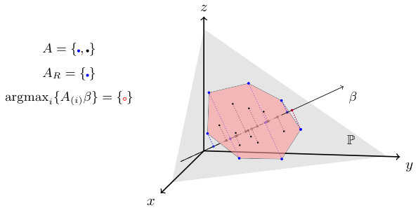 Figure 1
Peer Reviews
No public reviews on file for this paper yet. If you reviewed it on a platform where reviews are public (OpenReview, ICLR, NeurIPS, ICML), you can paste yours below so the community can read it here.
Videos
No videos yet. Explain this paper in a talk, walkthrough, or lecture? Add one.
11institutetext: 1CAS Key Lab of Network Data Science and Technology, Institute of Computing Technology, Chinese Academy of Sciences, 100190, Beijing, China
2University of Chinese Academy of Sciences, 100049, Beijing, China
3Centrum Wiskunde & Informatica and QuSoft, Science Park 123, 1098XG Amsterdam, Netherlands
{chenzhihuai,sunxiaoming,yuanpei}@ict.ac.cn,[email protected]
A Quantum-inspired Classical Algorithm for Separable Non-negative Matrix Factorization
Zhihuai Chen1,2
Yinan Li3
Xiaoming Sun1,2
Pei Yuan1,2
Jialin Zhang1,2
Abstract
Non-negative Matrix Factorization (NMF) asks to decompose a (entry-wise) non-negative matrix into the product of two smaller-sized nonnegative matrices, which has been shown intractable in general. In order to overcome this issue, separability assumption is introduced which assumes all data points are in a conical hull. This assumption makes NMF tractable and is widely used in text analysis and image processing, but still impractical for huge-scale datasets. In this paper, inspired by recent development on dequantizing techniques, we propose a new classical algorithm for separable NMF problem. Our new algorithm runs in polynomial time in the rank and logarithmic in the size of input matrices, which achieves an exponential speedup in the low-rank setting.
1 Introduction
Non-negative Matrix Factorization (NMF) aims to approximate a non-negative data matrix by the product of two non-negative low rank factors, i.e., , where is called basis matrix, is called encoding matrix and . In many applications, an NMF often results in more natural and interpretable part-based decomposition of data [LS99]. Therefore, NMF has been widely used in a number of practical applications, such as topic modeling in text, signal separation, social network, collaborative filtering, dimension reduction, sparse coding, feature selection and hyperspectral image analysis. Since computing an NMF is NP-hard [Vav09], a series of heuristic algorithms have been proposed [LS01, Lin07, HD11, KP08, DLJ10, GTLST12]. All of the heuristic algorithms aim to minimize the reconstruction error, the formula which is a non-convex program and lack optimality guarantee:
[TABLE]
A natural assumption on the data called separability assumption, was observed in [DS04] . From a geometry perspective, the separable assumption means that all rows of reside in a cone generated by a rather smaller number of rows. In particular, these generators are called anchors of . To solve the Separable Non-Negative Matrix Factorizations (SNMF), it is sufficient to identify the anchors in the input matrices, which can be solved in polynomial time [AGKM12, AGM12, GV14, EMO*+*12, ESV12, ZBT13, ZBG14]. Separability assumption is favored by various practical applications. For example, in the unmixing task in hyperspectral imaging, separability implies the existence of ‘pure’ pixel [GV14]. And in the topic detection task, it also means some words are associated with unique topic [Hof17]. In huge datasets, it is useful to pick up some representative data points to stand for other points. Such ‘self-expression’ assumption helps to improve the data analysis procedure [MD09, EV09].
1.1 Related work
It is natural to assume all the rows of the input has unit -norm, since -normalization translates the conical hull to convex hull while keeping the anchors unchanged. From this perspective, most algorithms essentially identify the extreme points in the convex hull of the (-normalized) data vectors. In [AGKM12], the authors use linear programs in variables to identify the anchors out of data points, and it is therefore not suitable for dealing with large-scale real-world problems. Furthermore, [RRTB12] presents a single LP in variables for SNMF to deal with large-scale problems (but is still impractical for huge-scale problems).
There is another class of algorithms based on greedy algorithms. The main idea is to opt a data point on the direction where the current residual decreases fast. The algorithms terminate with a sufficiently small error or a large iteration times. For example, Successful Projection Algorithm (SPA) [GV14] derives from Gram-Schmidt orthogonalization with row or column pivoting. XRAY [KSK13] detects a new anchor referring to the residual of exterior data points and updates the residual matrix by solving a nonnegative least square regression. Both of these two algorithms based on greedy pursuit have smaller time complexity compared with LP-based methods. However, the time complexity is still too large for large-scaled data.
[ZBT13, ZBG14] utilize a Divide-and-Conquer Anchoring (DCA) framework to tackle the SNMF. Namely, by projecting the data set into several low-dimension subspaces, and each projection can determines a small set of anchors. Moreover, it can be proven that all the anchors can be identified by projections.
Recently, a quantum algorithm for SNMF called Quantum Divide-and-Conquer Anchoring algorithm (QDCA), has been presented [DLL*+*18], which uses the quantum technology to speed up the random projection step in [ZBT13]. QDCA implements matrix-vector product (i.e., random projection) via quantum principal component analysis and then a quantum state encoding the projected data points could be prepared efficiently. Moreover, there are also several papers utilizing dequantizing techniques to solve some low-rank matrix operations, such as recommendation systems [Tan18] and matrix inversion [GLT18, CLW18]. Dequantizing techniques in those algorithms involve two technologies, the Monte-Carlo singular value decomposition and rejection sampling, which could efficiently simulate some special operations on low-rank matrices.
Inspired by QDCA and the dequantizing techniques , we propose a classical randomized algorithm which speeds up the random projection step in [ZBT13] and thereby identifies all anchors efficiently. Our algorithm takes time polynomial in rank , condition number and logarithm of the size of matrix. When rank , our algorithm achieves exponentially speedup than any other classical algorithms for SNMF.
1.2 Organizations
The rest of this paper is organized as follows: In Section 2, we introduce notations, models and preliminaries of our algorithm; in Section 3, we present our algorithm and analyze its correctness and running time; and Section 4 concludes with a discussion of this paper and the future work.
2 Preliminaries
2.1 Notations
Let . Let denote the space spanned by for . For a matrix , and denote the th row and the th column of for , respectively. Let where and (without loss of generality, assume ). and refer to Frobenius norm and spectral norm, respectively. For a vector , denotes its -norm. For two probability distributions (as density functions) over a discrete universe , the total variation distance between them is defined as . denotes the condition number of , where and are the maximal and minimal non-zero singular values of .
2.2 Sample Model
In query model, algorithms for SNMF problem require time which is at least linear in the number of nonzero elements of the matrix, since in the worst case, they have to read out all entries. However, we expect our algorithm to be efficient even if the datasets are extremely large. Considering the QDCA in [DLL*+*18], one of its advantage is that data is prepared in quantum state and can be access via ‘quantum’ way (like sampling). Thus, in quantum algorithm, quantum state is served to represent data implicitly which can be read out by measurement only. In order to avoiding reading the whole matrix, we introduce a new sample model other than the query model based on the idea of quantum state preparation assumption.
Definition 1 (-norm Sampling)
Let denote the distribution over with density function for . A sample from a distribution is called a sample from .
Lemma 1 (Vector Sample Model)
There is a data structure storing vector in space, and supporting following operations:
- •
Querying and updating a entry in time;
- •
Sampling from in time;
- •
Finding in time.
Such a data structure can be easily implemented via Binary Search Tree (BST) (see Figure 1).
Proposition 1 (Matrix Sample Model)
Considering matrix , let and be the vector whose entry is and , respectively. There is a data structure storing matrix in space and supporting following operations:
- •
Querying and updating an entry in time;
- •
Sampling from for any in time ;
- •
Sampling from for any in time ;
- •
Finding , and in time ;
- •
Sampling and in time and , respectively.
This data structure can be easily implemented via Lemma 1, we can just use two arrays of BST to store all rows and columns of and use two extra BSTs store and .
2.3 Low-rank Approximations in Sample Model
FKV algorithm is a Monte-Carlo algorithm [FKV04] that returns approximate singular vectors of given matrix in matrix sample model. The low-rank approximation of can be reconstructed by approximate singular vectors. The query and sample complexity of FKV algorithm are independent of size of . FKV algorithm outputs a short ‘description’ of , which is approximate to a right singular vectors of matrix . Similarly, FKV algorithm can output a description of approximate left singular vectors of by inputting . Let FKV () denote the FKV algorithm, where is a matrix given by sample model, is the rank of approximate matrix of , is error parameter, and is the failure probability. The FKV algorithm is described in Theorem 2.1.
Theorem 2.1 (Low-rank Approximations, [FKV04])
Given matrix in matrix sample model, and , FKV algorithm outputs the description of the approximate right singular vectors in samples and queries of with probability , which satisfies
[TABLE]
Especially, if is a matrix with rank exactly, Theorem 2.1 also implies an inequality:
[TABLE]
Description of .
Note that FKV algorithm does not output the approximate right singular vectors directly since their lengths are linear of . It returns a description of , which consists of three components: the row index sets , a vector set which are singular vectors of a submatrix sampled from , and its corresponding singular values , where . In fact, for . Given a description of , we can sample from in time for [Tan18] and query its entry in time .
Definition 2 (-orthonormal)
Given , is called -approximately orthonormal if for and for .
The next lemma presents some properties of -approximate orthonormal vectors.
Lemma 2 (Properties of -orthonormal Vectors, [Tan18])
Given a set of -approximately orthonormal vectors , then there exists a set of orthonormal vectors spanning the columns of such that
[TABLE]
where represents the orthonormal projector to image of and are constants.
Lemma 3 ([FKV04])
The output vectors of is -approximate orthonormal.
3 Fast Anchors Seeking Algorithm
In this section, we present a randomized algorithm for SNMF which is called Fast Anchors Seeking (FAS) Algorithm. Especially, the input of FAS is given by matrix sample model which is realized via a data structure described in Section 2. FAS returns the indices of anchors in time polynomial logarithmic to the size of matrix.
3.1 Description of Algorithm
Recall that SNMF aims to factorize where is the index set of anchors. In this paper, an additional constraint is added: the sum of entries in any row of is 1. Namely, any data point of resides in convex hull which is the set of all convex combination of . In fact, normalizing each row of matrix by -norm is valid, since the anchors remain unchanged. Moreover, Instead of storing -normalized matrix , we can just maintain the -norms for all rows and columns.
The Quantum Divide-and-Conquer Anchoring (QDCA) is a quantum algorithm for SNMF which achieves exponential speedup than any classical algorithms [DLL*+*18]. After projecting any convex hull into an 1-dimensional space, the geometric information is partially preserved. Especially, the anchors in 1-dimensional projected subspace are still anchors in the original space. The main idea of QDCA is quantizing random projection step in DCA. It decomposes SNMF into several subproblems: projecting onto a set of random unit vectors with , i.e., computing . Such a matrix-vector product can be efficiently implemented by Quantum Principle Component Analysis (QPCA). And then it returns a -qubits quantum state whose amplitudes are proportional to entries of . Measurement of quantum state outcomes an index which obeys distribution . Thus, we can prepare copies of quantum states, measure each of them in computational basis and record the most frequent index. By repeating procedure above with times, we could successively identify all anchors with high probability.
As discussed above, the core and most costly procedure is to simulate . At the first sight, traditional algorithms can not achieve exponential speedup on account of limits of computational model. In QDCA, vectors are encoded into quantum states and we can sample the entries with probability proportional to their magnitudes by measurements. This quantum state preparation overcomes the bottleneck of traditional computational model. Based on divided-and-conquer scheme and sample model (See Section 2.2), we present Fast Anchors Seeking (FAS) Algorithm inspired by QDCA. Designing FAS is quite hard and non-trivial although FAS and QDCA have the same scheme. Indeed, we can simulate directly by rejection sampling technology. However, the number of iterations of rejection sampling is unbounded. To overcome this difficulty, we translate matrix into its approximation , where the columns consists of approximate left singular vectors of matrix and . Next, it is obvious that is a short vector and we can estimate its entries one by one (see Lemma 7) efficiently. Now the problem becomes to simulate and it can be done by Lemma 6 .
Given an error parameter , the method described above will result in via Theorem 2.1, which implies . Namely, the method above introduces an unbounded error in form if is arbitrary vector in entire space . Fortunately, this issue can be solved by generating random vectors lying in row space of instead of those lying in entire space . To generate uniform random unit vectors on the row space of , we need to find a basis of row space of . If is a set of orthonormal basis of the row space of (the space spanned by the right singular vectors), and is uniform random unit vector on , then is a unit random vector in row space of . Moreover, FKV algorithm will figure out approximate singular vectors for , that can help us make an approximate for . Therefore, we will estimate distribution instead of . Based on Corollary 7, can be estimated efficiently. According to Lemma 6, can be sampled efficiently, thus we can treat as estimation of (see Figure 2).
Once we can simulate distribution , we can figure out the index of the largest component of vector by picking up samples (Theorem 3.2). Moreover, according to [ZBT13], by repeating this procedure with times, we can find all anchors of with high probability (For single step of random projection, see Figure 3).
3.2 Analysis
Now, we propose our main theorem and analyze the correctness and complexity of our algorithm FAS.
Theorem 3.1 (Main Result)
Given separable non-negative matrix in matrix sample model, the rank , condition number and a constant , Algorithm 1 returns the indices of anchors with probability at least in time
[TABLE]
3.2.1 Correctness
In this subsection, we will analyze the correctness of Algorithm 1. Firstly, we show that the columns of defined in Lemma 2 form a basis of row space of matrix , which is necessary to generate unit vector in row space of . The next, we prove that for each , distribution is -close to distribution in total variant distance. Once again, we show how to gain the index of largest component of from distribution . Finally, by random projection, it is enough for us to gain all anchors of matrix .
The following lemma tells us the approximate singular vectors outputted by FKV spans the row space of matrix . And combining with Lemma 2, it gives us that also spans the same space, i.e., forms an orthonormal basis of row space of matrix .
Lemma 4
Let be the output of algorithm . If , then with probability , we obtain
[TABLE]
Proof
By contradiction, we assume that , which implies that there exists a unit vector and . Then we can obtain since . And according to Theorem 2.1, we have
[TABLE]
Thus , which makes a contradiction if .
By Lemma 4, we can generate an approximate random vector in the row space of with probability in time by FKV (). Firstly, we obtain the description of approximate right singular vectors by FKV algorithm, where the error parameter is bounded by rank and condition number (see in Lemma 4). Secondly, we generate a random unit vector as a coordinate vector referring to a set of orthonormal vectors in Lemma 2. Let denotes the matrix defined in Lemma 2, then it is obvious that its columns form the right singular vectors for matrix . That is, is an approximate vector of a random vector . Next, we show that total variant distance between and is bounded by constant . For convenience, we assume that each step in Algorithm 1 succeeds and the final success probability will be given in next subsection.
Lemma 5
For all , holds simultaneously with probability .
In the rest, without ambiguity, we use notations , instead of , . By applying triangle inequality, we divide the left part of inequality into four parts (the intuition idea please ref Figure 2):
[TABLE]
Thus, we only need to prove that ①, ②, ③, ④ , respectively. In addition, given , if , then . For ①, ② and ③, we only show their -norm version, i.e.,
- •
;
- •
;
- •
.
For convenience, in the rest part, let and represent approximate ratio for orthonormality of and based on Lemma 3, respectively.
Before we start our proof, we list two tools which are used to prove ③ and ④, respectively.
Based on rejection sampling, Lemma 6 shows that sampling from linear combination of -approximately orthogonal vectors can be quickly realized without knowledge of norms of these vectors (see Algorithm 2).
Lemma 6 ([Tan18])
Given a set of -approximately orthonormal vectors in vector sample model, and an input vector , there exists an algorithm outputting a sample from a distribution -close to with probability using queries and samples.
Lemma 7
Given in matrix sample model and and in query model, let , then we can output a matrix , with probability , such that
[TABLE]
by queries and samples.
Proof
Let with and . In [Tan18], there exists an algorithm that outputs an estimation of () to precision with probability in time . Let . We can output with probability utilizing queries and samples respectively where satisfies
[TABLE]
Proof (proof of Lemma 5)
Upper bound for ①. By Lemma 4, is a unit random vector sampled from the row space of with probability if . From Eq. (1) in Lemma 2, with probability
[TABLE]
Combing with , we gain
[TABLE]
Eq. (3) satisfies with .
Upper bound for ②. According to Lemma 4, the columns of span a space equal to the column space of if with probability . Let denote the orthonormal projector to image of (column space of ). Similarly, denotes the orthonormal projector to the orthogonal space of column space of .
[TABLE]
based on Eq. (2) in Lemma 2. If , .
Upper bound for ③. When and are discussed above, with probability , we have
[TABLE]
According to Lemma 7, we obtain
[TABLE]
Combining Eq. (5) and Eq. (6), the following holds
[TABLE]
If , then holds.
Upper bound for ④. Since as discussed before, directly taking usage of Lemma 6, with probability we have
[TABLE]
Hence, Algorithm 1 generates a distribution which satisfies for random unit vectors generated simultaneously with probability .
The following theorem tells us how to find the largest component of from distribution .
Theorem 3.2 (Restatement of Theorem 1 in [DLL*+*18])
Let be a distribution over and is another distribution simulating with total variant error . Let be examples independently sampled from and be the number of examples taking value of . Let and . If , then, for any , with a probability at least , we have
[TABLE]
As mentioned in [DLL*+*18], the assumption about the gap between and is easy to satisfy in practice. By choosing and , we have , which will converge to zero as goes to infinity.
To estimate the number of random projections we need, we denote the probability that after random projection , a data point is identified as an anchor in subspace, i.e.,
[TABLE]
In [ZBG14], if for a constant , with random projections, all anchors can be found with probability at least .
3.2.2 Complexity and Success Probability
Note that Algorithm 1 involves operations that query and sample from matrix , and , but those operations can be implemented in time. Thus, in the following analysis, we just ignore the time complexity of those operations but multiple it to the final time complexity.
The running time and failure probability mainly concentrates on lines 4, 6, 7 and 11 in Algorithm 1. The running time of lines 4 and 6 are and , respectively, according to Theorem 2.1. And line 7 takes to estimate matrix according to Lemma 7. And line 11 with iterations totally spends . In the perspective of failure probability, lines 4, 6 and 7 take the same failure probabilities . And line 11 takes for each iteration.
Above all, the time complexity of FAS is . The success probability is .
4 Conclusion
This paper presents a classical randomized algorithm FAS which dramatically reduces the running time to find anchors of low-rank matrix. Especially, we achieve exponential speedup when the rank is logarithmic of the input scale. Although our algorithm running in polynomial of logarithm of matrix dimension, it still has a bad dependence on rank . In the future, we plan to improve its dependence on rank as well as analyze its noise tolerance.
The reference list from the paper itself. Each links out to its DOI / PubMed record.
- 1[AGKM 12] Sanjeev Arora, Rong Ge, Ravindran Kannan, and Ankur Moitra. Computing a nonnegative matrix factorization–provably. In Proceedings of the forty-fourth annual ACM symposium on Theory of computing , pages 145–162. ACM, 2012.
- 2[AGM 12] Sanjeev Arora, Rong Ge, and Ankur Moitra. Learning topic models–going beyond svd. In Foundations of Computer Science (FOCS), 2012 IEEE 53rd Annual Symposium on , pages 1–10. IEEE, 2012.
- 3[CLW 18] Nai-Hui Chia, Han-Hsuan Lin, and Chunhao Wang. Quantum-inspired sublinear classical algorithms for solving low-rank linear systems. ar Xiv preprint ar Xiv:1811.04852 , 2018.
- 4[DLJ 10] Chris HQ Ding, Tao Li, and Michael I Jordan. Convex and semi-nonnegative matrix factorizations. IEEE transactions on pattern analysis and machine intelligence , 32(1):45–55, 2010.
- 5[DLL + 18] Yuxuan Du, Tongliang Liu, Yinan Li, Runyao Duan, and Dacheng Tao. Quantum divide-and-conquer anchoring for separable non-negative matrix factorization. In Proceedings of the 27th International Joint Conference on Artificial Intelligence , pages 2093–2099. AAAI Press, 2018.
- 6[DS 04] David Donoho and Victoria Stodden. When does non-negative matrix factorization give a correct decomposition into parts? In Advances in neural information processing systems , pages 1141–1148, 2004.
- 7[EMO + 12] Ernie Esser, Michael Moller, Stanley Osher, Guillermo Sapiro, and Jack Xin. A convex model for nonnegative matrix factorization and dimensionality reduction on physical space. IEEE Transactions on Image Processing , 21(7):3239–3252, 2012.
- 8[ESV 12] Ehsan Elhamifar, Guillermo Sapiro, and Rene Vidal. See all by looking at a few: Sparse modeling for finding representative objects. In 2012 IEEE Conference on Computer Vision and Pattern Recognition , pages 1600–1607. IEEE, 2012.