Estimating the division rate from indirect measurements of single cells
Marie Doumic (MAMBA), Ad\'ela\"ide Olivier (UP11 UFR Sciences), Lydia, Robert (MICALIS)

TL;DR
This paper investigates how to estimate the division rate of bacteria based on indirect measurements of size, providing a theoretical reconstruction formula and demonstrating its effectiveness through numerical simulations and experimental data.
Contribution
It introduces a method to estimate division rates from size data within the adder model, including a reconstruction formula and numerical validation.
Findings
Reconstruction of division rate is feasible despite ill-posedness.
Numerical methods yield satisfactory results on simulated data.
Application to experimental data confirms practical utility.
Abstract
Is it possible to estimate the dependence of a growing and dividing population on a given trait in the case where this trait is not directly accessible by experimental measurements, but making use of measurements of another variable? This article adresses this general question for a very recent and popular model describing bacterial growth, the so-called incremental or adder model. In this model, the division rate depends on the increment of size between birth and division, whereas the most accessible trait is the size itself. We prove that estimating the division 10 rate from size measurements is possible, we state a reconstruction formula in a deterministic and then in a statistical setting, and solve numerically the problem on simulated and experimental data. Though this represents a severely ill-posed inverse problem, our numerical results prove to be satisfactory.
Click any figure to enlarge with its caption.
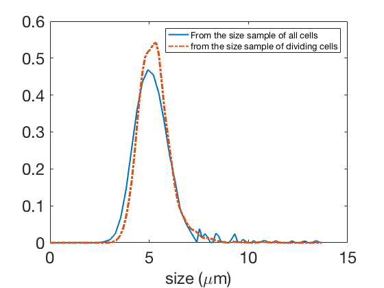 Figure 1
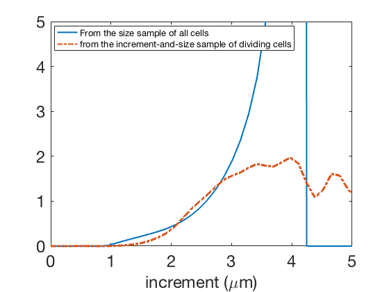 Figure 2
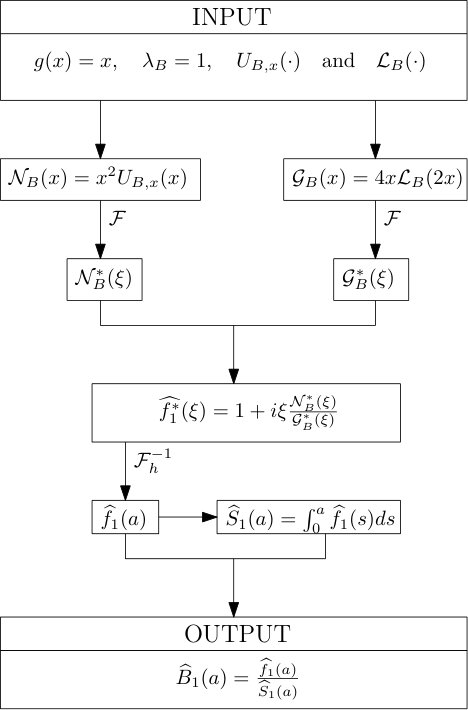 Figure 3
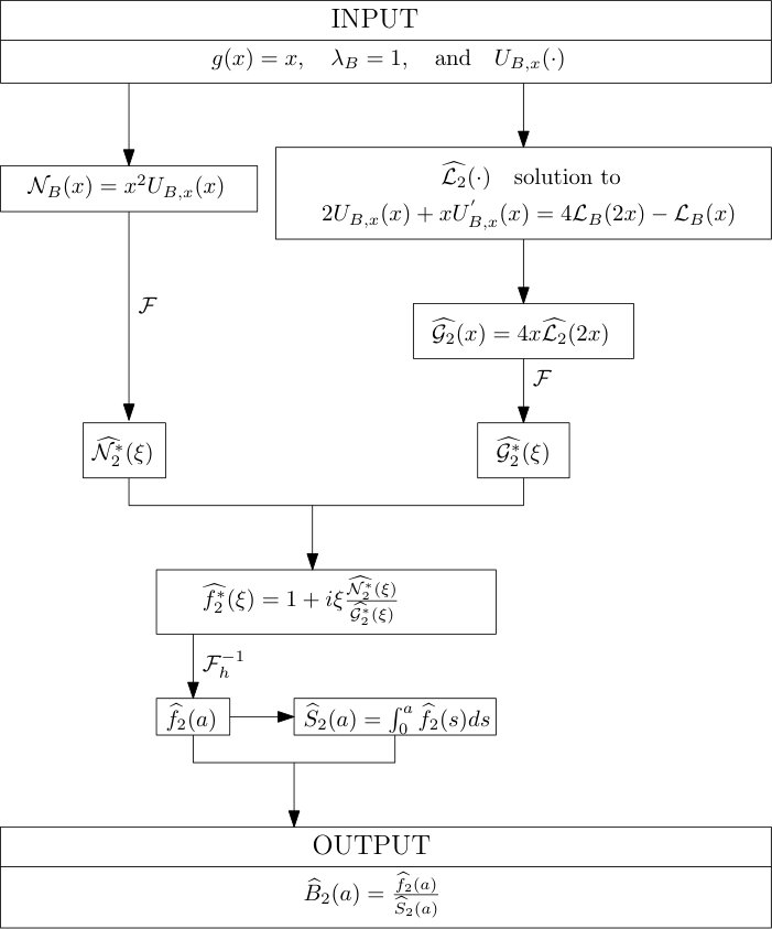 Figure 4
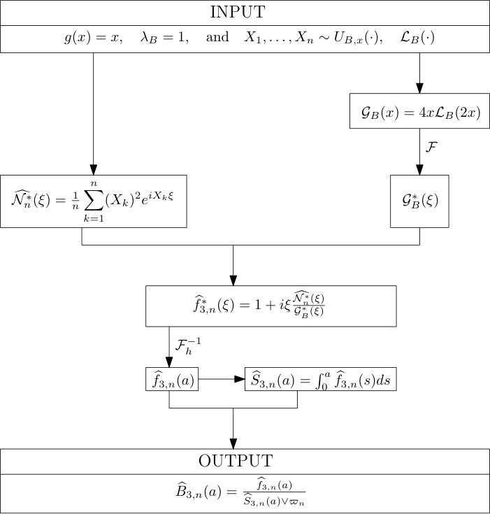 Figure 5
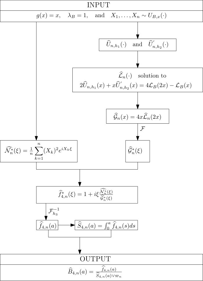 Figure 6
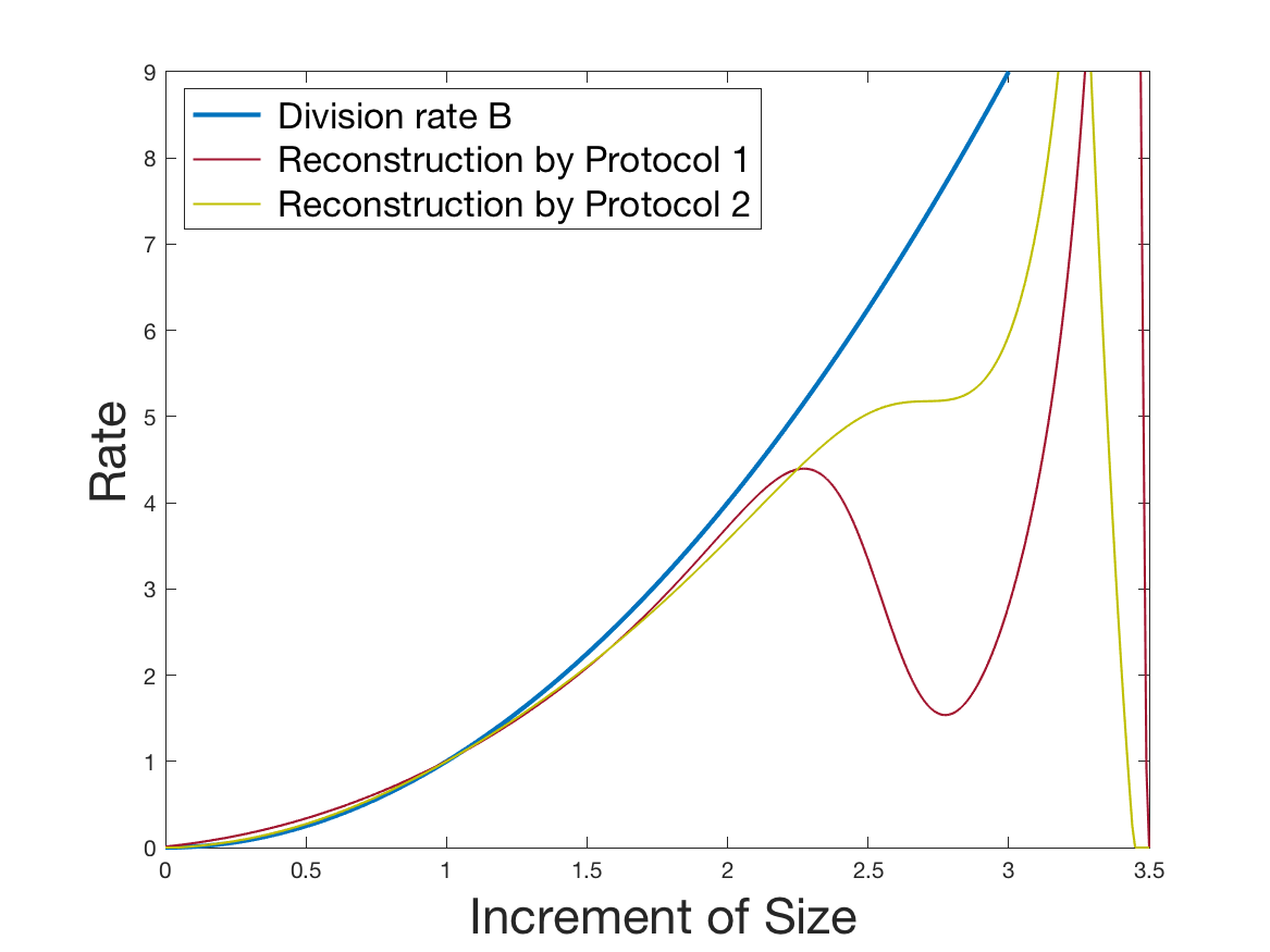 Figure 7
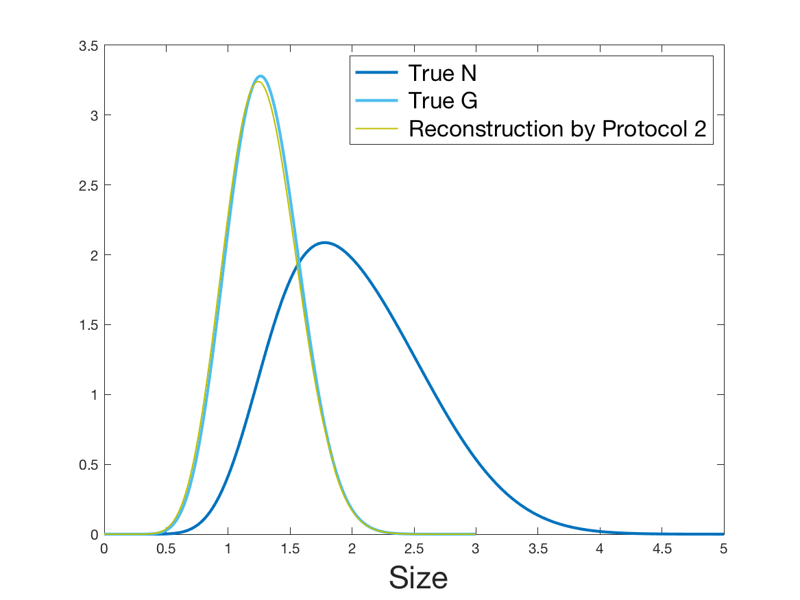 Figure 8
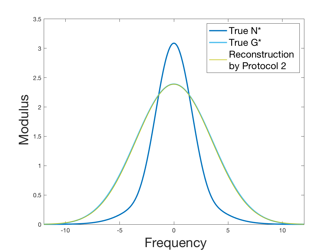 Figure 9
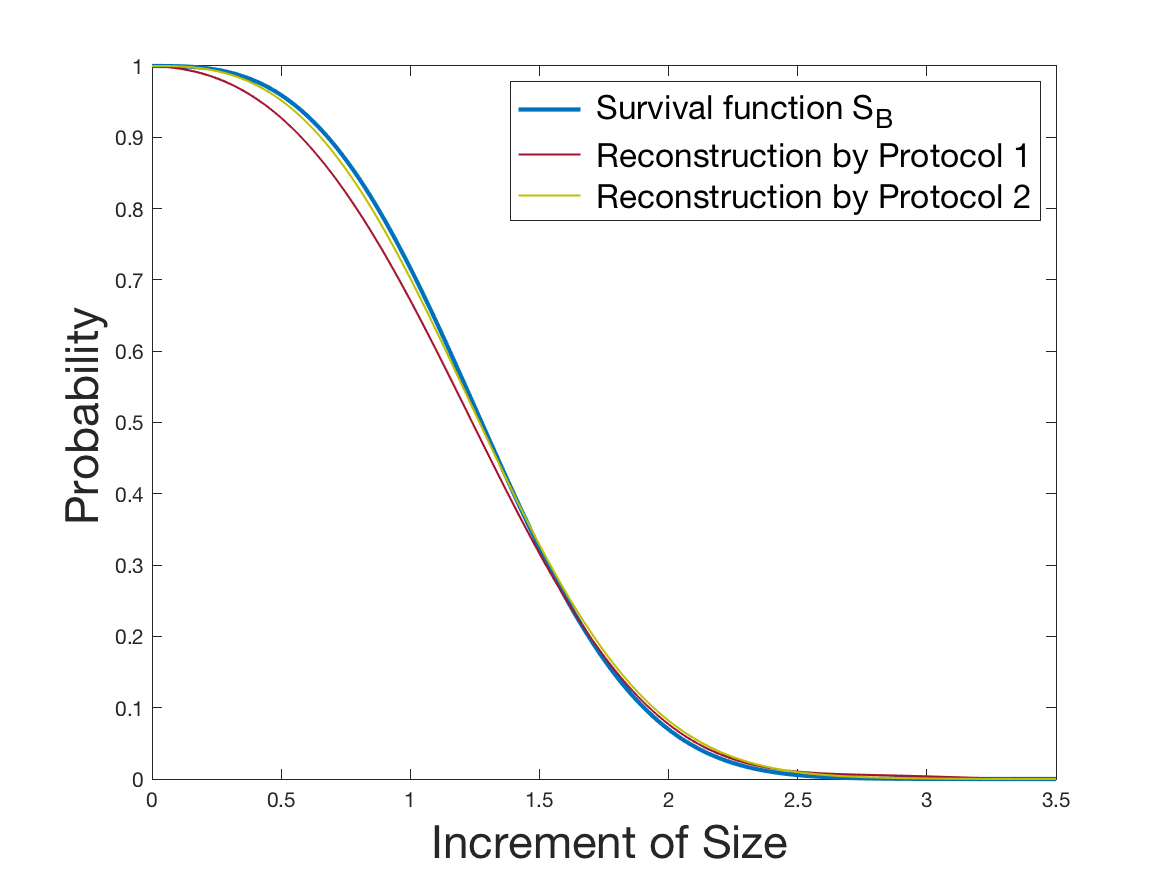 Figure 10
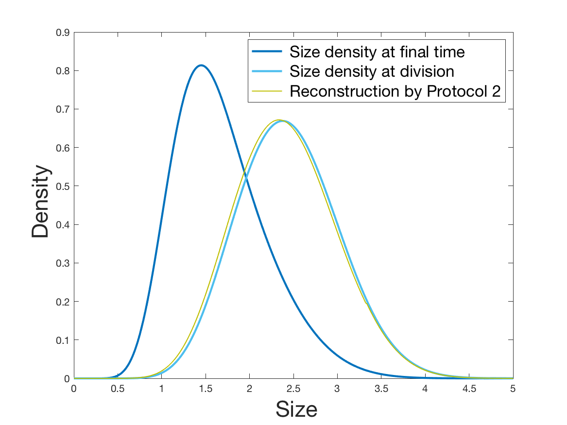 Figure 11
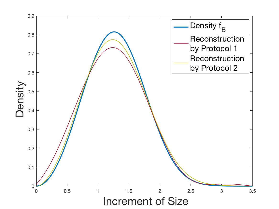 Figure 12
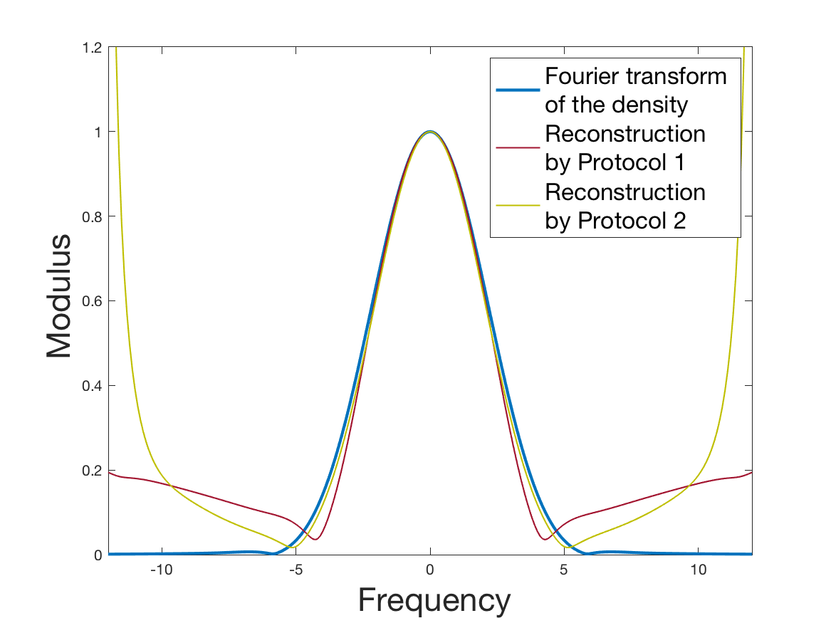 Figure 13
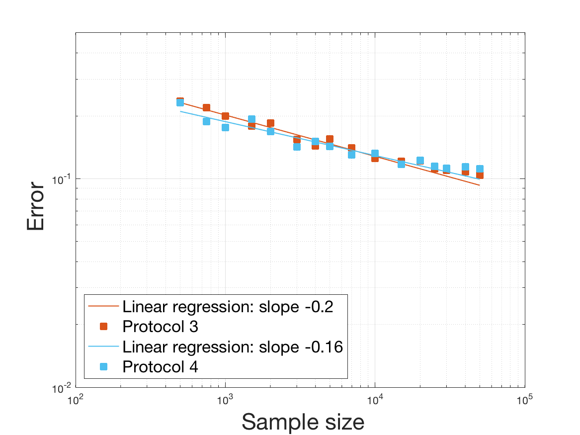 Figure 14
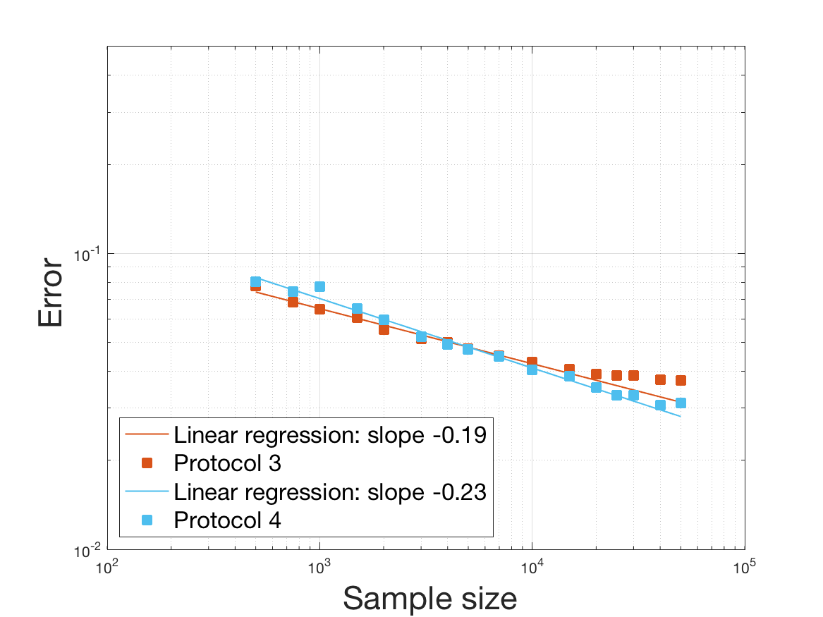 Figure 15
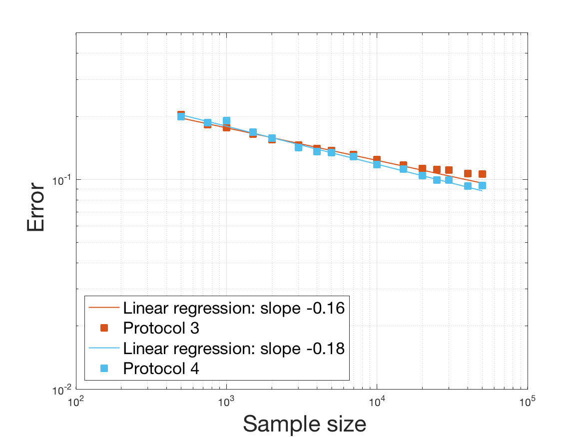 Figure 16
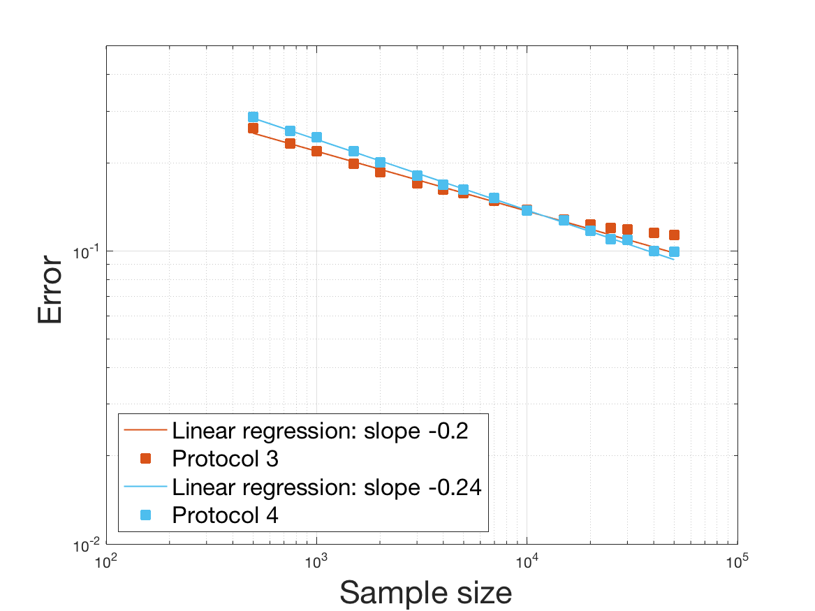 Figure 17
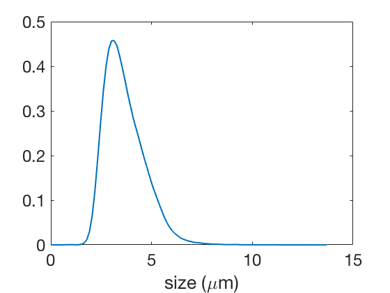 Figure 18
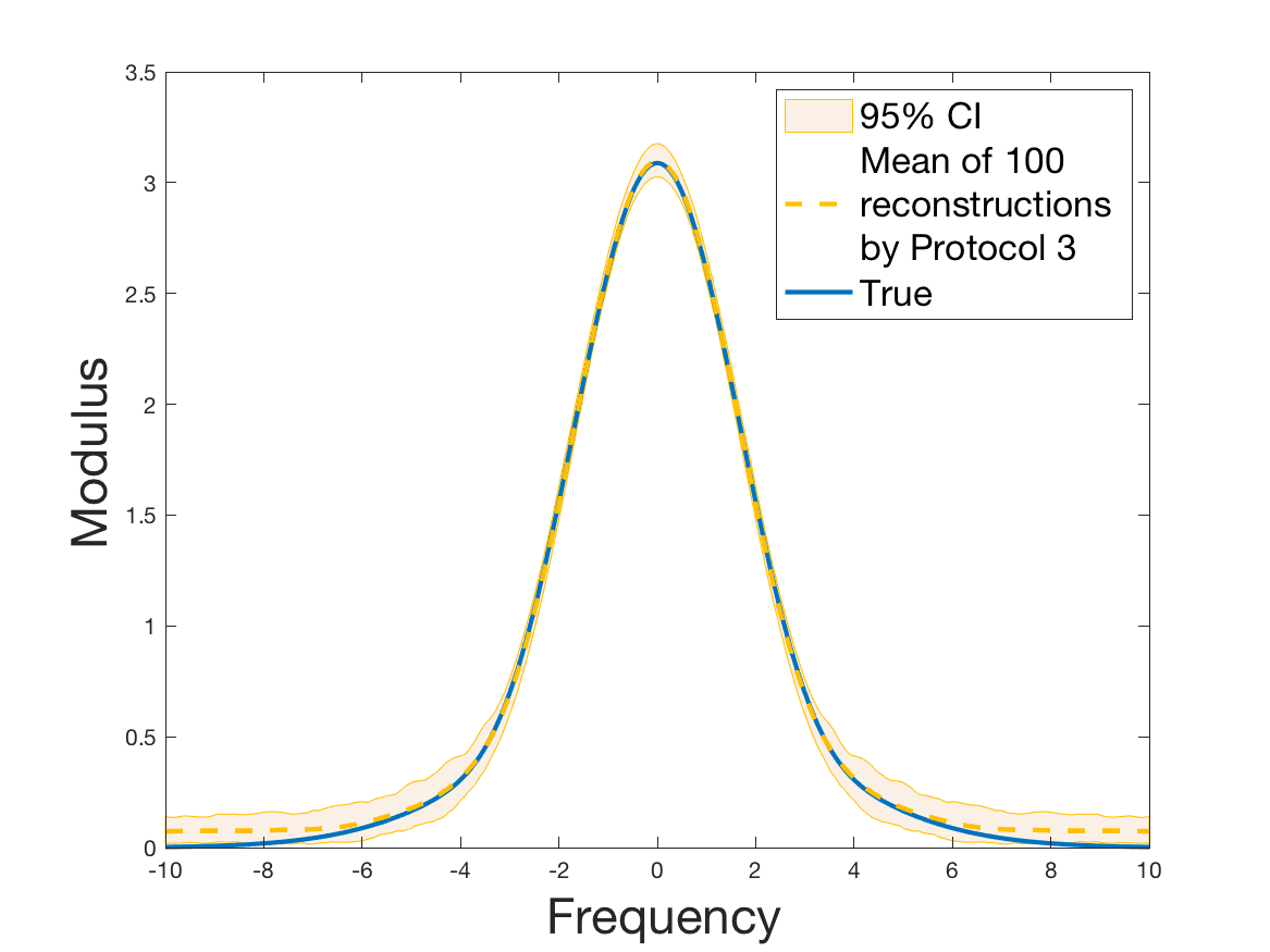 Figure 19
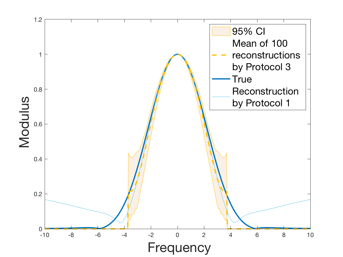 Figure 20
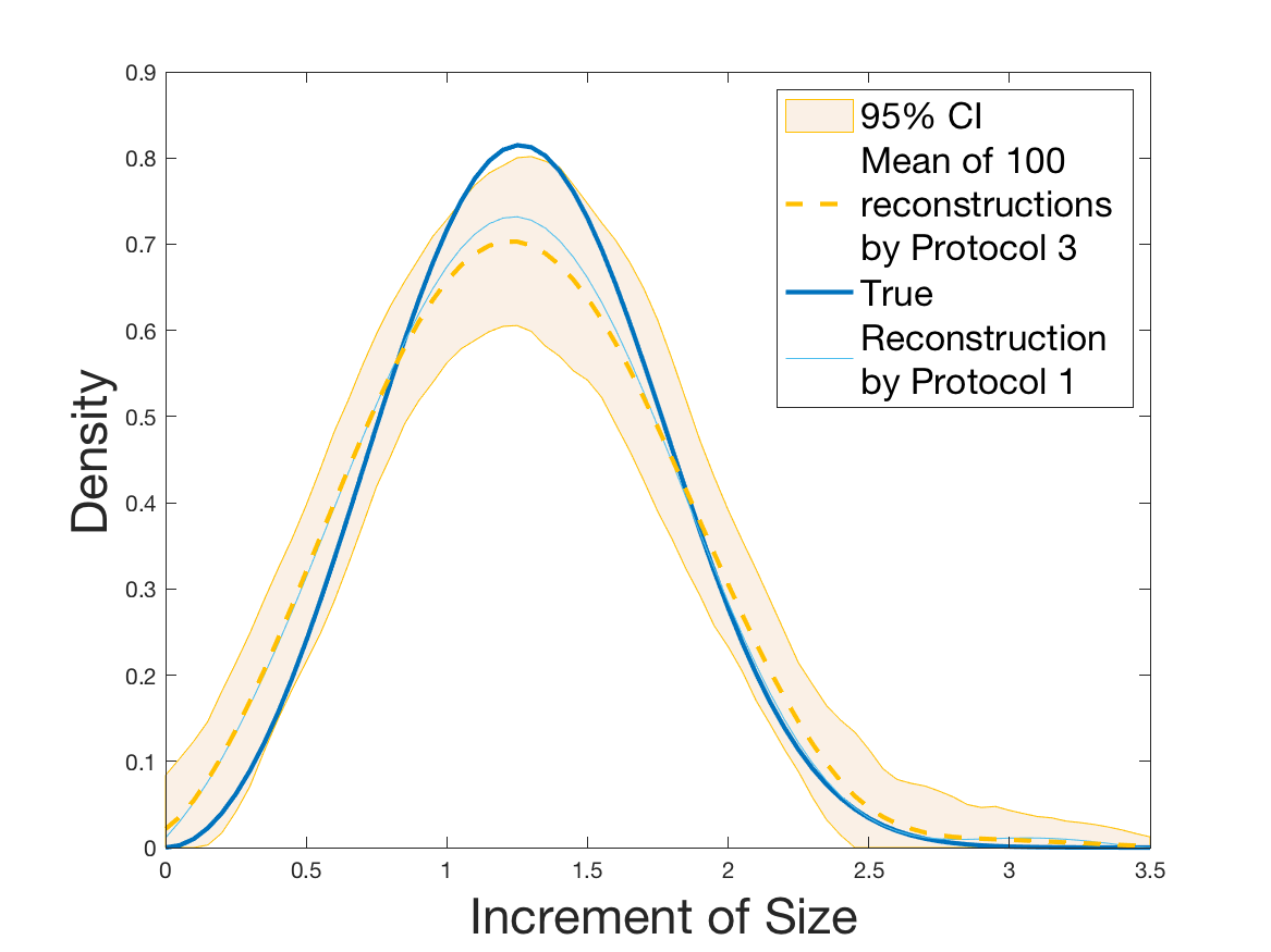 Figure 21
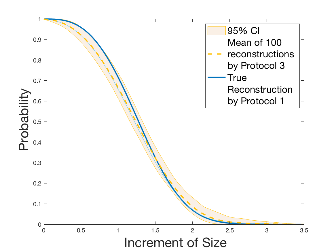 Figure 22
 Figure 23
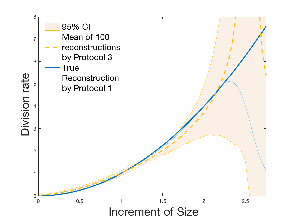 Figure 24
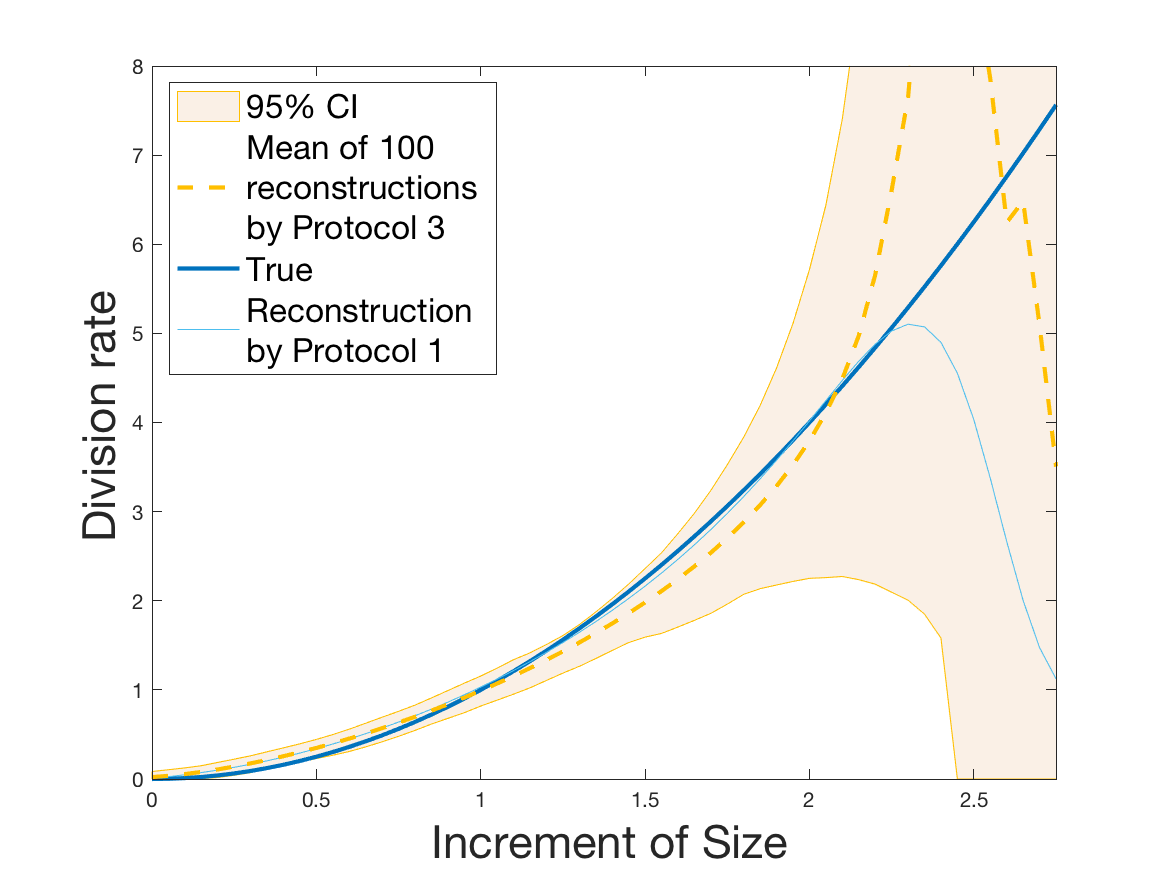 Figure 25
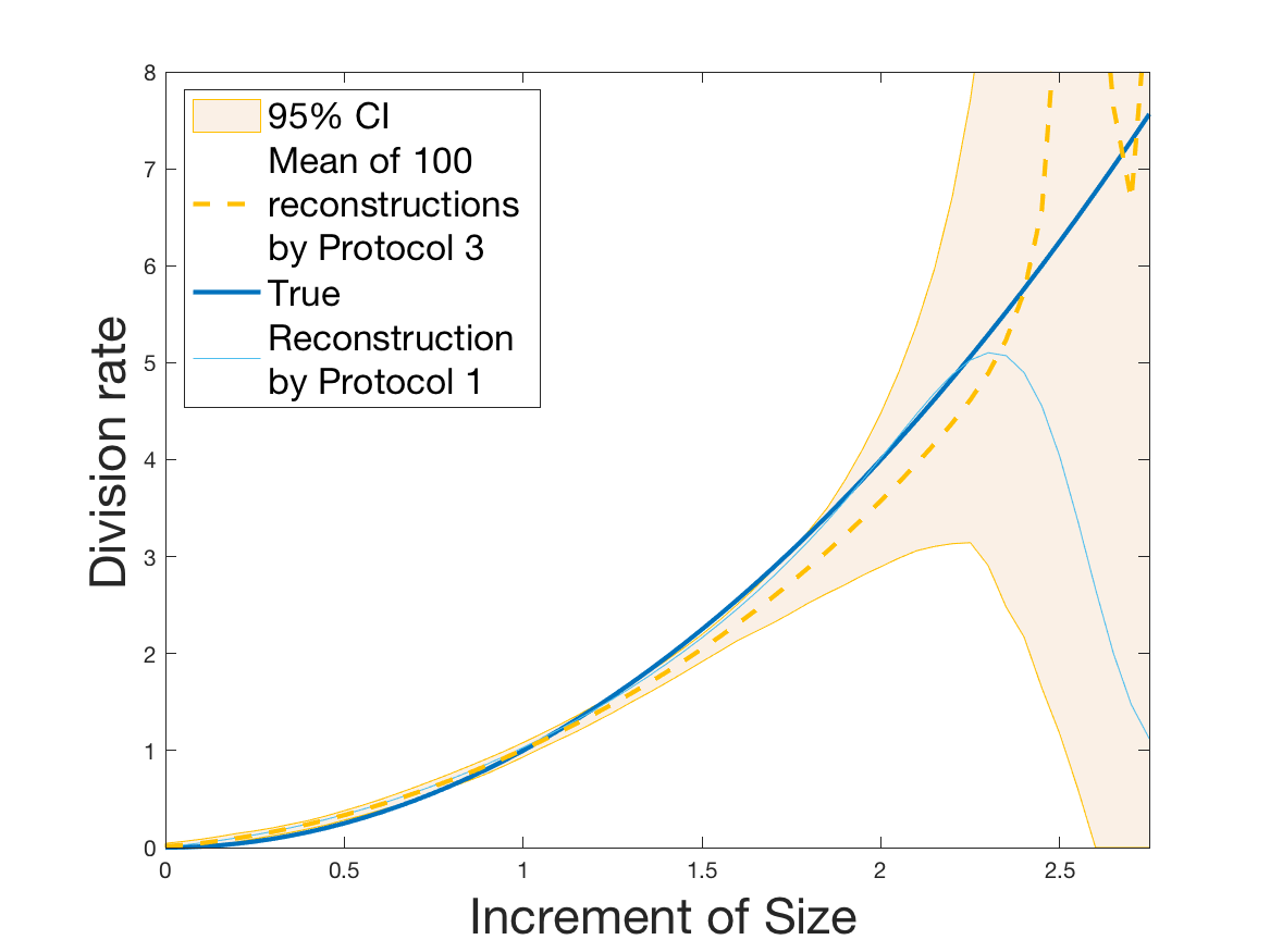 Figure 26
 Figure 27
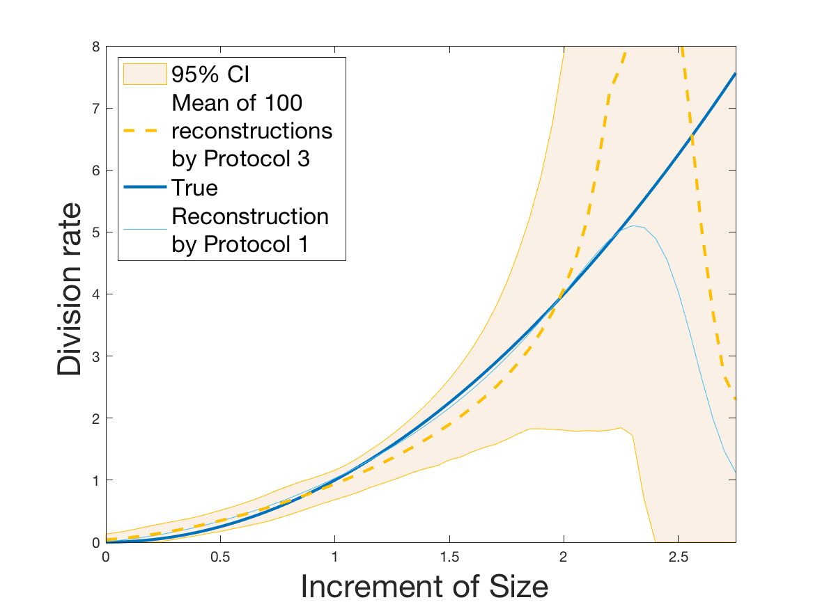 Figure 28
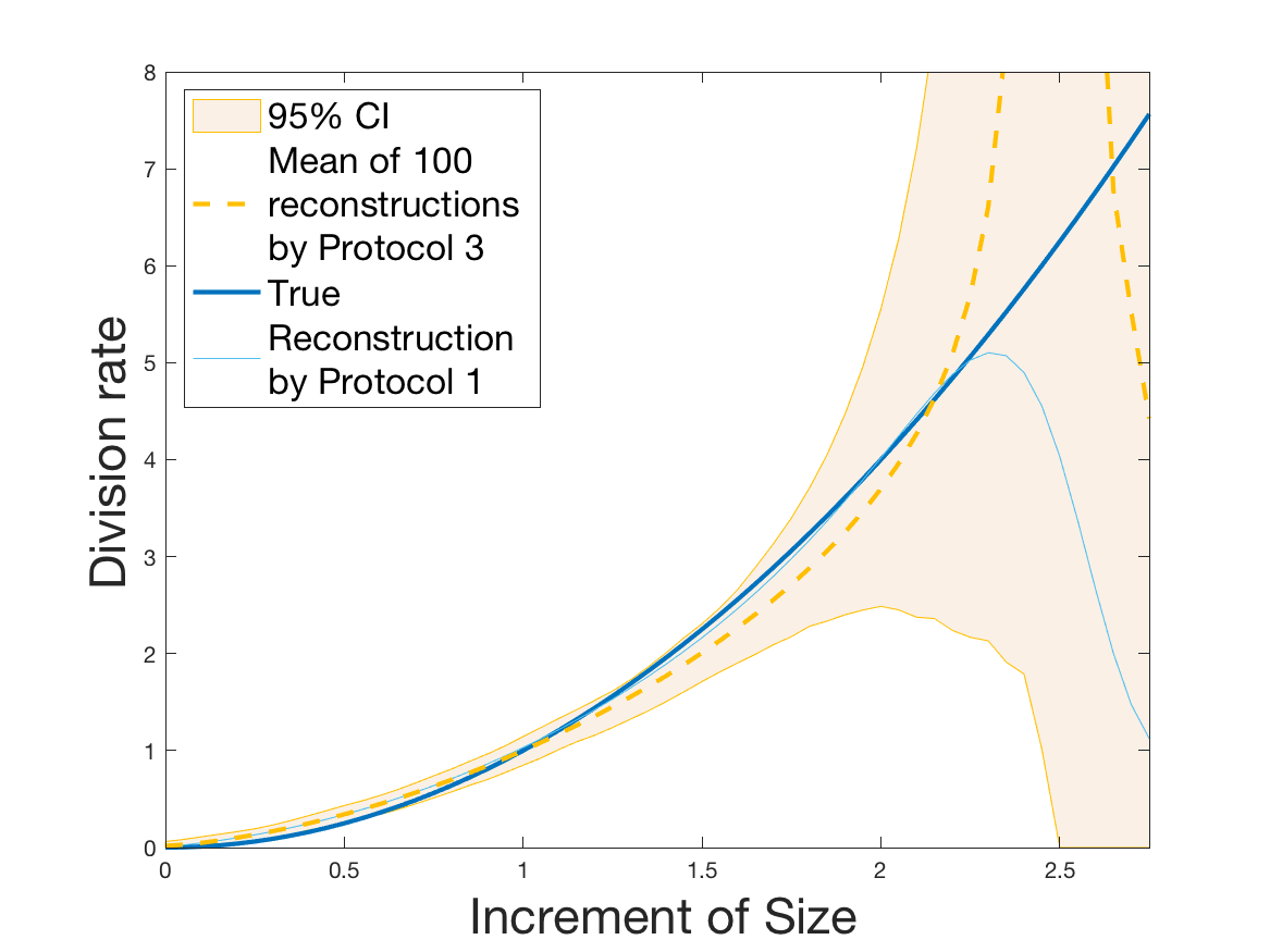 Figure 29
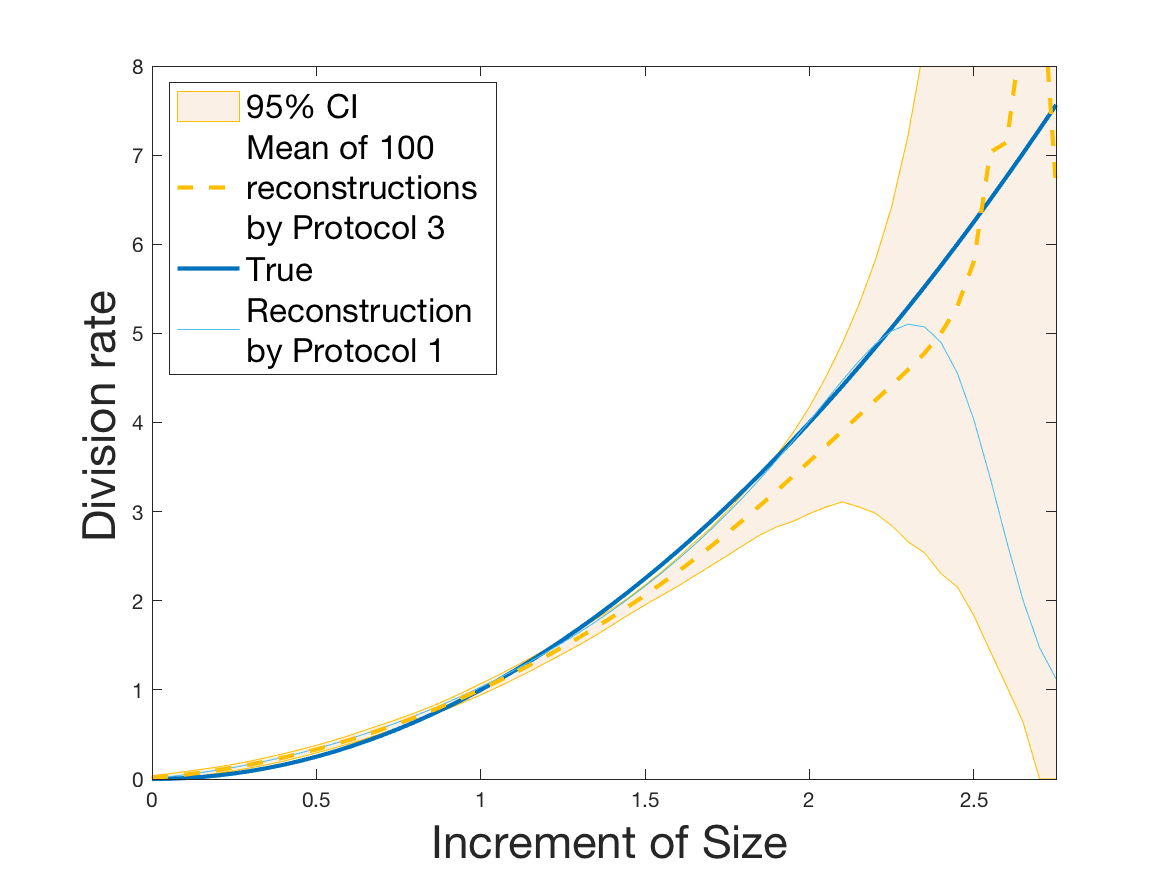 Figure 30
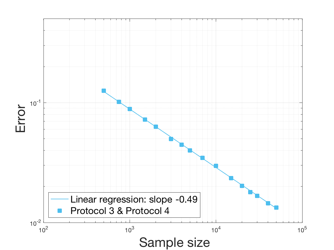 Figure 31
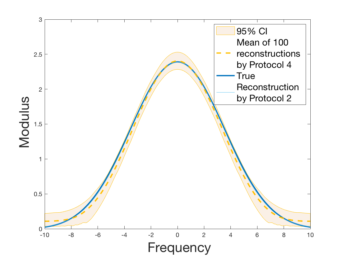 Figure 32
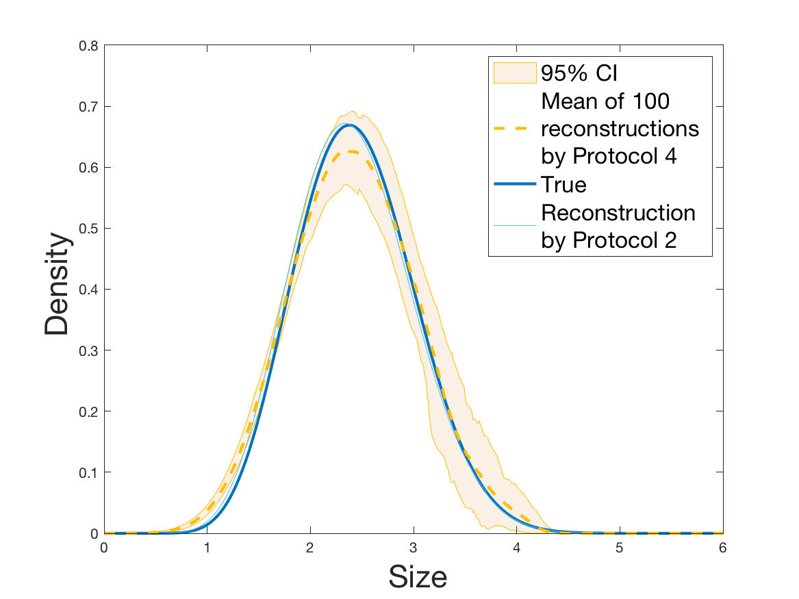 Figure 33
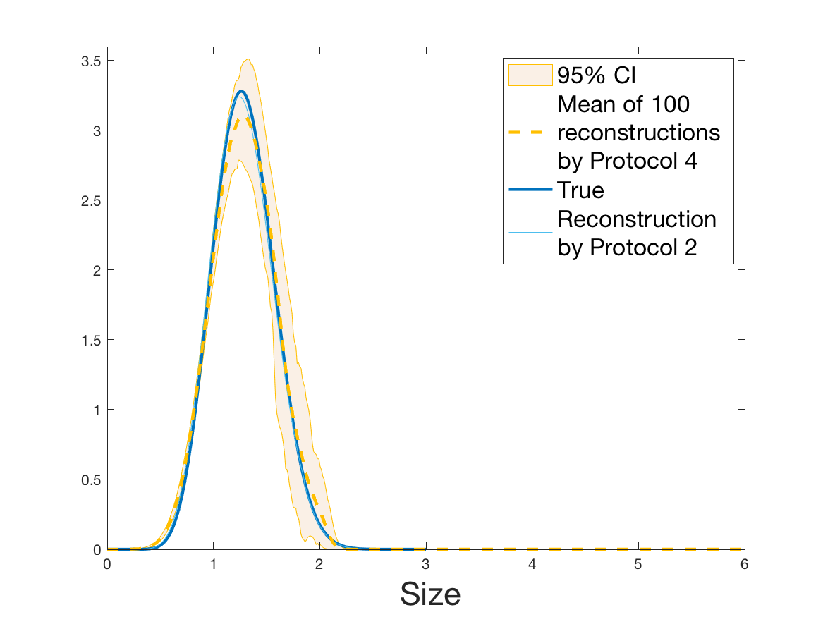 Figure 34
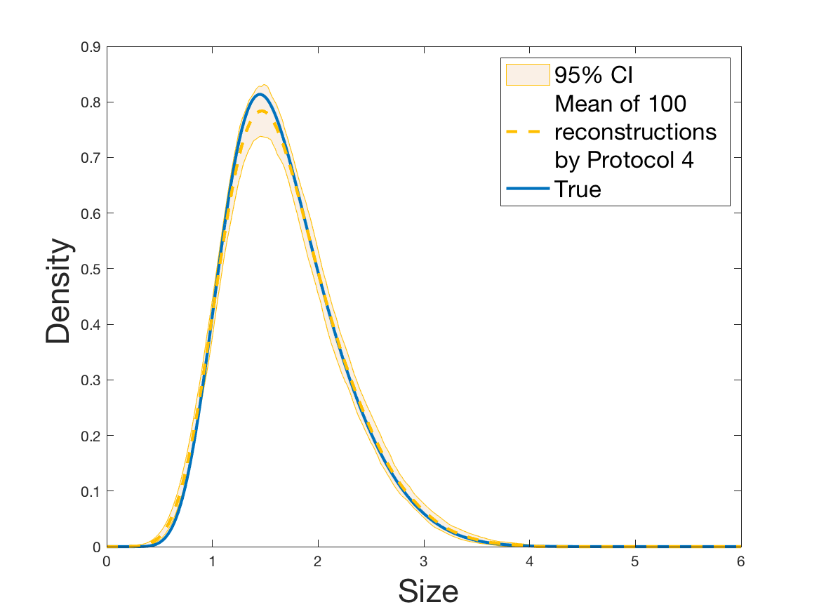 Figure 35
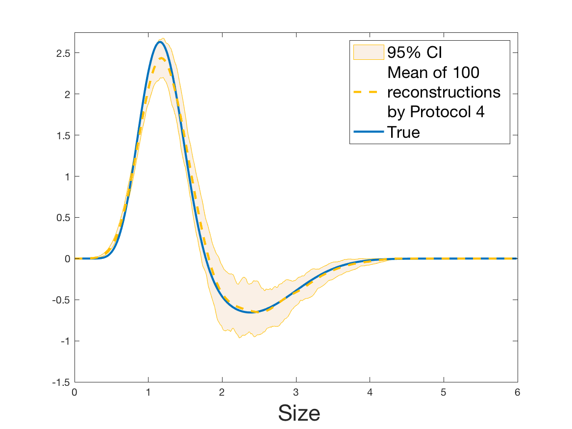 Figure 36
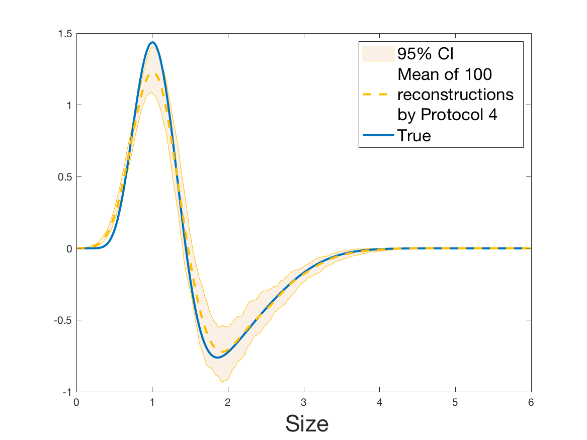 Figure 37
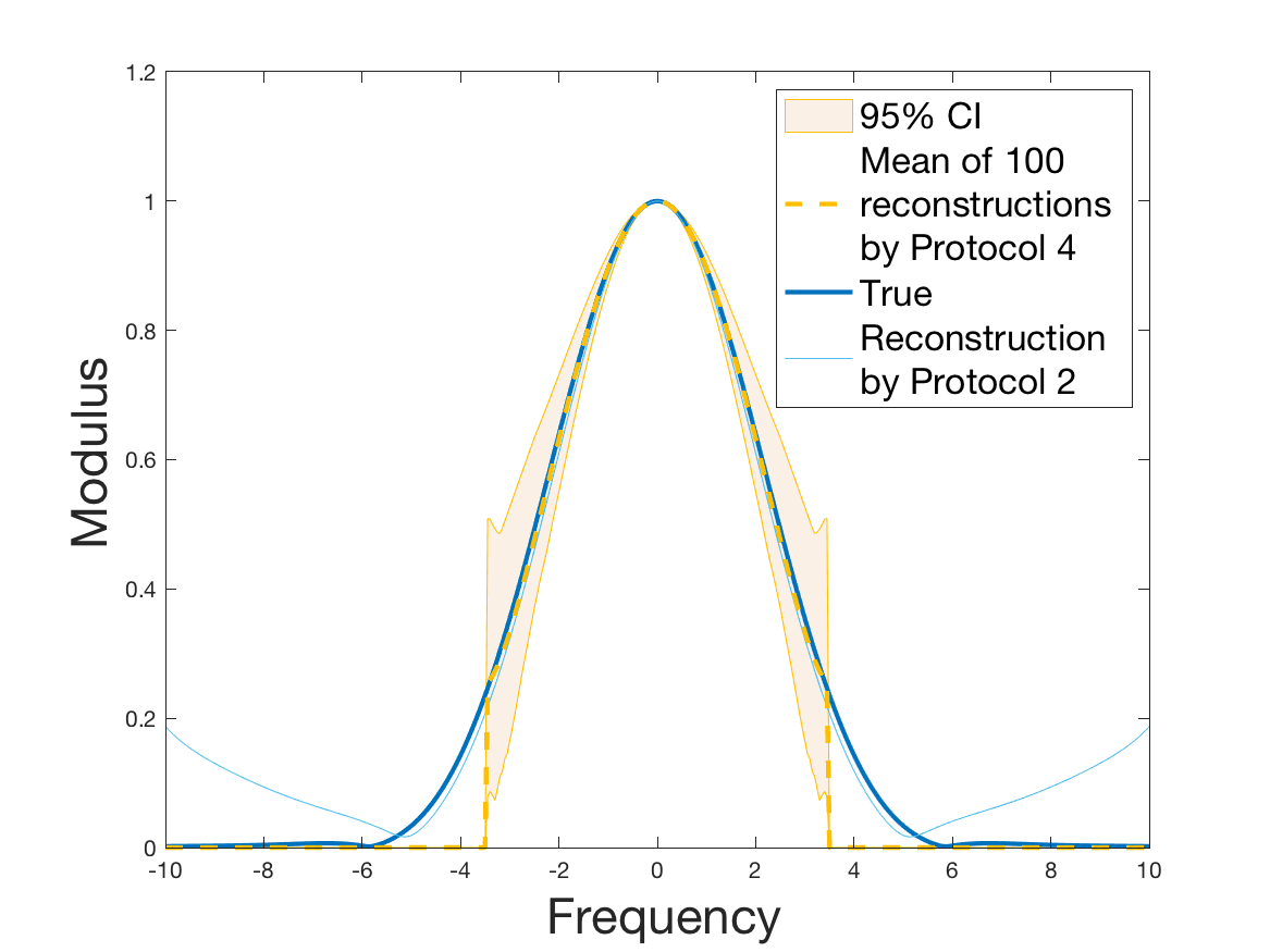 Figure 38
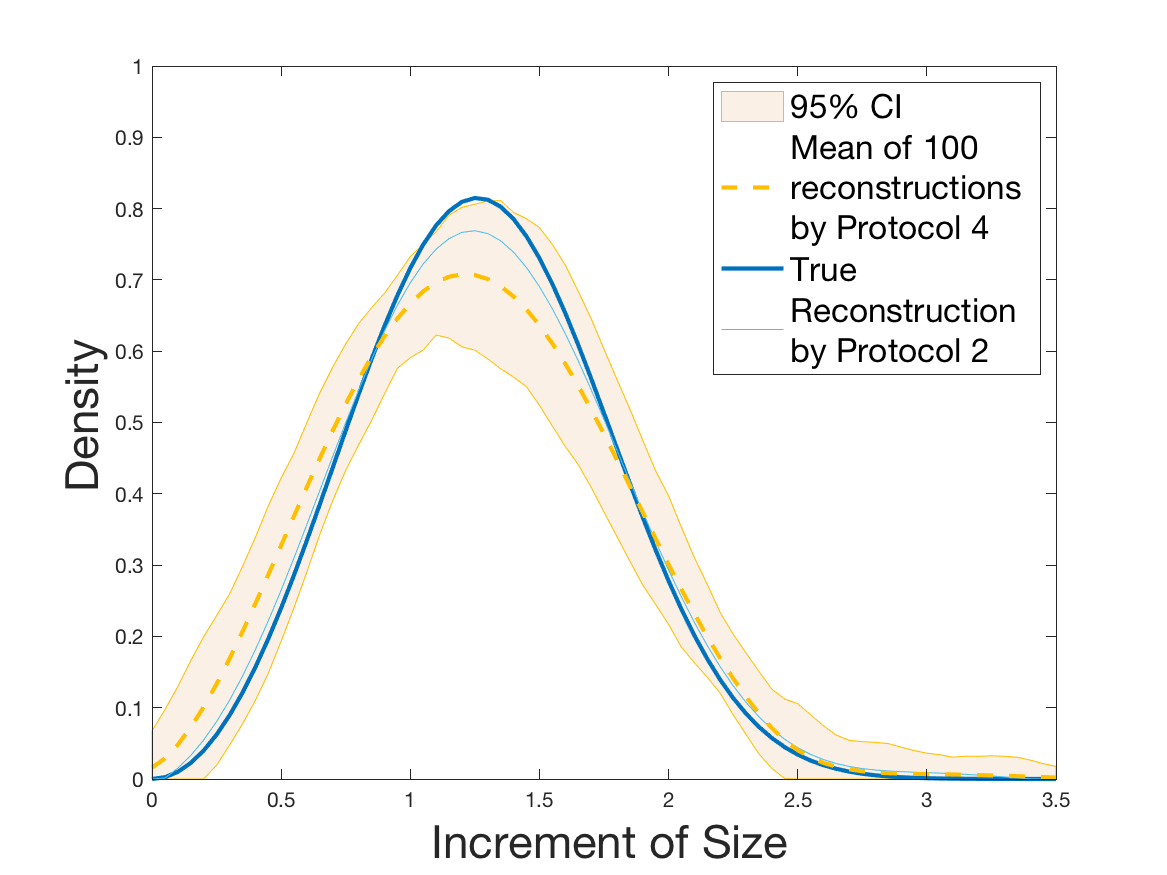 Figure 39
 Figure 40
| Reconstruction of | ||||||
|---|---|---|---|---|---|---|
| Numerical | [0;6] | [0;6] | [-50;50] | [0;5] | [0;5] | |
| sampling | ||||||
| Protocol 1 | - | - | - | 0.1062 | 0.1043 | 0.0395 |
| Protocol 2 | 0.0478 | 0.0417 | 0.0417 | 0.0470 | 0.0482 | 0.0149 |
| Reconstruction of | ||
|---|---|---|
| Numerical | [0;2] | [0;2.5 ] |
| sampling | ||
| Protocol 1 | 0.0730 | 0.2065 |
| Protocol 2 | 0.0849 | 0.1321 |
Peer Reviews
No public reviews on file for this paper yet. If you reviewed it on a platform where reviews are public (OpenReview, ICLR, NeurIPS, ICML), you can paste yours below so the community can read it here.
Videos
No videos yet. Explain this paper in a talk, walkthrough, or lecture? Add one.
Taxonomy
TopicsListeria monocytogenes in Food Safety · Mathematical and Theoretical Epidemiology and Ecology Models · Bacterial Genetics and Biotechnology
Estimating the division rate from indirect measurements
of single cells
Marie Doumic111Sorbonne Université, Inria, Université Paris-Diderot, CNRS, Laboratoire Jacques-Louis Lions, F-75005 Paris, France. Email adress: [email protected]
Adélaïde Olivier222Laboratoire de Mathématiques d’Orsay, Univ. Paris-Sud, CNRS, Université Paris-Saclay, 91405 Orsay, France. Email adress: [email protected]
Lydia Robert
Abstract
Is it possible to estimate the dependence of a growing and dividing population on a given trait in the case where this trait is not directly accessible by experimental measurements, but making use of measurements of another variable? This article adresses this general question for a very recent and popular model describing bacterial growth, the so-called incremental or adder model. In this model, the division rate depends on the increment of size between birth and division, whereas the most accessible trait is the size itself. We prove that estimating the division rate from size measurements is possible, we state a reconstruction formula in a deterministic and then in a statistical setting, and solve numerically the problem on simulated and experimental data. Though this represents a severely ill-posed inverse problem, our numerical results prove to be satisfactory.
Introduction
The field of structured population equations has attracted much interest for more than sixty years, leading to substantial progress in their mathematical understanding. These equations describe a population dynamics in terms of well-chosen traits, which offer a relevant characterization of the individual behaviour. More recently, thanks to considerable progress in experimental measurements, the question of estimating the parameters from single-cell measurements also attracts a growing interest, since it finally allows comparing models model and data, and thus investigating which variable is biologically relevant as a structuring variable - see for instance [30] for the application to age-structured and size-structured models for bacterial growth.
However, the so-called structuring variable of the model may be quite abstract (”maturity”, ”satiety”…), and/or not directly measurable, whereas the quantities that are effectively measured may be linked to the structuring one in an unknown or intricate manner. As an illustration of this idea, we can cite the interesting series of articles by H.T. Banks and co-authors, concerning the estimation of the division rate in data sets where the measured quantity was the fluorescence (carboxyfluorescein succinimidyl ester (CFSE)) of the cells. Initially, they designed a fluorescence-structured model [2], but then the estimated division rates appeared difficult to interpret biologically. Indeed, the fluorescence was artificially added to the cells, thus it was not structuring: the difficulty was to find out which variable was really structuring, and how it was related to the measured quantities. This was done successfully by this group by building a model structured in both the true structuring variable - the so-called ”cyton model” - and in the label, i.e. the measured quantity [3].
From such considerations we can formulate a general question: is it possible to estimate the dependence of a population on a given variable, which is not experimentally measurable, by taking advantage of the measurement of another variable?
In this article, we address this question in a specific setting, namely the growth and division of bacteria. Recently, it was evidenced that for several types of bacteria and yeast cells, the ”increment of size”, i.e. the increase of size of a cell between its birth and its division, provides a better-fitted model than age- or size-structured models [9, 17, 19, 33]. These studies were based on data obtained by time-lapse microscopy and consisting in measurements of single-cells growing and dividing. Such data allows estimating for each cell its lifetime, its size at birth and at division, and its size-evolution through time. We refer to this kind of data as ”measurements of dividing cells”.
Comparison of models and data, such as performed in the above-mentioned studies, requires time-lapse microscopy data obtained in finely controlled conditions ensuring stable, steady-state growth. In addition, precise image analysis is also required to obtain accurate size measurements of numerous single-cells. Obtaining such data is therefore not straight-forward and can be time-consuming. This can represent an important limitation, for instance for screening strategies where data has to be obtained in many different bacterial strains or experimental conditions. Here we consider the case of data consisting only in instantaneous size measurements of single-cells in a population. Such measurements can be more easily obtained, by microscopy snapshots, or using a flow cytometer or a coulter counter which both allow high-throughput acquisition.
From such data, the question of estimating the division rate in a size-structured model has been studied in a series of papers, in a deterministic [6, 16, 29] or statistical [15] setting. The rates of convergence for the estimates have been proved to correspond to an inverse problem of degree of ill-posedness one, hence worse than the rate of convergence obtained from measurements of dividing cells (corresponding, in a deterministic setting, to a degree of ill-posedness zero, see [14] for a discussion of this heuristics).
In view of the new biological evidence in favour of the incremental model [8, 10, 17, 31, 33], this article is devoted to the same question as in [29] and following articles, but for the incremental model: Can we estimate an increment-dependent division rate from a measurement of the size-distribution of cells? Though formulated in a similar way, this new problem is much more complex, since the observed variable (instantaneous size) is not the structuring variable (size increment).
Let us now give a mathematical definition of the problem under study. First of all, we recall the increment-structured model.
The incremental model for bacterial growth
Let us denote the density of cells at time of size which have an increment between their actual size and their size at birth . We denote this increment as it may be viewed as a kind of age, since it increases monotonically and starts at zero at birth - but an age that would have a link with the size: if denotes the growth rate of a cell of size , its ”aging rate” is also We have the following increment-and-size model, as proposed in Taheri-Araghi et al. [33] for bacteria, and also designed in a different context by Hall et al. in [22] :
[TABLE]
The instantaneous probability to divide is, as in [22], for a cell of size-increment and size . From a modelling point of view, writing the division rate as the product of and a function allows us to interpret as the instantaneous probability to divide in a unit of growth instead of a unit of time. This is coherent with the fact that the cell may ignore the ”time” and use its growth as a clock. As will be explained below, in the case proposed by Taheri-Araghi et al. [33] where , this is also coherent with a much simpler and more natural underlying piecewise deterministic Markov process (PDMP), where the time of division is a simple renewal process of jump rate , so that the increments of dividing cells are mutually independent and distributed according to the density f_{B}(a)=B(a)\exp\big{(}-\int\limits_{0}^{a}B(s)ds\big{)}.
Asymptotic behaviour of the incremental model
Under suitable assumptions on the coefficients and (for instance the theorem 3.7. of [11] may be adapted and provides a proof for smooth growth and division rates, and most recently [20] studies the case , with fairly general division rate ), we have a dominant eigentriplet unique solution of
[TABLE]
Moreover, using for instance the general relative entropy inequalities, we have under some more assumptions (theorem 4.5. in [11])
[TABLE]
Let us however notice that under the assumption made in [33], namely that this precise asymptotic behaviour fails to happen and a cyclic behaviour is observed, as already proved for the growth-fragmentation equation [5, 21]. This corresponds to an idealised case; in reality, there is always some variability, leading to a growth slightly different from perfectly exponential and to a division into two slightly unequal parts, see for instance [30]. From a numerical perspective, this slight ”imperfection” has to be included, else the cyclic behaviour will perturb the results, see Section 3 for more details.
Mathematical formulation of the inverse problem
From now on, we denote by to underline the dependence in the unknown division rate. Let us assume that we measure the steady size-distribution, which is modeled by the marginal . Such a measurement may be done for instance via a sample of cells for which we measure their sizes assumed to be the realization of an i.i.d. sample distributed along in the spirit of Doumic, Hoffmann, Reynaud-Bouret and Rivoirard [15].
We also assume division into two equally-sized daughters, as modelled in (1), and that and are already known from an independent measurement or previous knowledge. Typically, may be measured through the time evolution of the total mass, which is classical in biology [27], and under the consensual assumption of exponential growth , we have In this article, we do not consider the noise in the measurement of and which could be included in future work.
The problem we want to solve in order to have a fully determined model is:
Given \big{(}\lambda,g(\cdot)\big{)} and given measurements of
can we estimate the division rate ?
In Section 2, we provide an explicit though intricate formula for the estimation of from , without taking the noise into account. We then provide a statistical estimator in Section 2, numerically implemented in Section 3 both on simulated data and real data. These numerical results provides us with clues concerning directions for future work, which we comment in the discussion (Section 4).
1 Reconstruction formula in a deterministic setting
Before providing the reconstruction formula for let us introduce some useful notation. As standard in the field of renewal processes, we introduce the probability distribution function and the survival function of the increments of dividing cells:
[TABLE]
Symetrically, we introduce the size-distribution of dividing cells, that we denote
[TABLE]
As shown below, the function is an important intermediate to formulate from the measurement of Though we cannot write it as an explicit function of it can be obtained in a similar way as the distribution of dividing cells for the size-structured equation, see [16].
Lemma 1**.**
Let be a positive continuous function on , and a positive function on such that with . Then there exists a unique solution such that
[TABLE]
and there exists such that
[TABLE]
If moreover there exists solution of the system (3)-(4) such that then this unique solution coincides with the size-distribution of dividing cells defined by (8).
Proof. The existence, uniqueness and continuity part directly follows from [16] Proposition A.1. If is solution to (3)-(4) , we integrate Equation (3) along the increment , use the boundary condition (4), and obtain Equation (9) with defined by (8).
With this lemma, we see that the estimation of from is an inverse problem of degree of ill-posedness 1 when stated in a space (degree 3/2 in the framework of a statistical noise [15, 28]), as already known from [29]. Interestingly, we remark that this would remain true also if the division rate would depend on other structuring variables, as soon as the growth rate and the division kernel are known: this allows one to reconstruct the size distribution of dividing cells from the size distribution of all cells, in any framework.
We are now ready to formulate in terms of , and the parameters and This is done in the next proposition.
In all what follows, we denote by the Fourier transform of a function :
[TABLE]
Proposition 1**.**
Let and be such that there exists a unique positive eigentriplet solution of the eigenproblem (3)–(6). Let us furthermore assume and define as the unique solution of Equation (9) given by Lemma 1.
We define and by (7). We define two intermediate functions and by
[TABLE]
with an anti-derivative of We assume that and are the well-defined Fourier transforms of and .
We have the following reconstruction formula for in terms of and
[TABLE]
provided that all the inverse Fourier transforms are well defined and that neither nor the denominator vanishes.
Corollary 1**.**
Under the assumptions of Proposition 1, if we have , and
Remark 1**.**
At this stage, the reconstruction formula is formal: to give it a rigorous meaning and ensure its validity, we would have to prove that all the quantities are well-defined, in particular that the Fourier transform never vanishes. This requires a full study per se, and is beyond the scope of this work: in another case study, this has been done for instance for the estimation of the fragmentation kernel of the growth-fragmentation equation in the article [13], using the Cauchy integral to prove that a Mellin transform never vanishes, proof adapted to another case in [23]. For these two cases however, the proofs used strongly an explicit formulation of the solution with the use of Mellin or Fourier transforms, thanks to the fact that was a power law in [13], and constant in [23]. We let it for future work.
Proof. The aim is to use the classical formula and to find a formulation for in terms of , then express as its integral.
First step. Formulating in terms of , and .
As done for the study of the eigenvalue problem carried out for instance in [11, 20], we can classically obtain a formulation of in terms of We first write Equation (4) under the form
[TABLE]
and then use the method of characteristics to solve (3) and (12). We define an intermediate function solution of
[TABLE]
we define \tilde{C}(a,x)=C(a,x+a)e^{\int\limits_{0}^{a}\bigl{(}\frac{\lambda}{g(x+s)}+B(s)\bigr{)}ds}, which satisfies so that
[TABLE]
which gives for :
[TABLE]
using (12) for the last equality. We integrate the equation (13) in and obtain
[TABLE]
Second step. Formulating two deconvolution problems for and .
Denoting by an antiderivative of , and defining an intermediate function the previous formula is equivalent to
[TABLE]
We define by (10), thus Equation (14) is nothing but
[TABLE]
This is a deconvolution problem, where is the unknown. If we find estimators of and , we can reconstruct . Since integrating by parts we can transform (15) into a deconvolution problem for .
Third step. Solution of the deconvolution problems by Fourier transform.
Extending all the functions on by zero (with a slight abuse of notation, we keep the same notation for the function and for its extension), we rewrite (15) in the Fourier domain, and for such that :
[TABLE]
Since is a probability density for which we assume continuity around [math] and we can extend it continuously by [math] on , we have and and since for we get
[TABLE]
for such that . The expresses the Fourier transform of the discontinuity of the prolongation of in since ; however, this term should be compensated by since we have assumed .
Fourth step. Inverse Fourier transforms. and are given by the formulae
[TABLE]
provided all these quantities exist, and we have proved the formula (11).
Remark 2**.**
An alternative formula for would be obtained using a direct formula for the survival function,
[TABLE]
2 Statistical setting: estimation procedure
Let us assume that we have a sample independent and identically distributed according to . This idealizes the case where, for instance, a picture of all individuals at a given time is taken, and their sizes experimentally measured. We give here a procedure to estimate from such a sample.
2.1 Estimation of
Step 1. Estimation of by a kernel estimator
[TABLE]
with . Estimation of D(y)=\big{(}gU_{B,x}\big{)}^{\prime}(y) by
[TABLE]
For the choice of the regularization parameters and , see Section 3.
Step 2. Inversion of (9) replacing the left-hand side by . We obtain an estimator of . For this step, we follow [6], and concatenate the inverse given in Lemma 1 in for , that we denote , with the inverse in , denoted , for for a given (to be determined numerically) : we set
[TABLE]
Step 3. We deduce an estimator of using its definition (10):
[TABLE]
2.2 Estimation of the Fourier transforms and
Estimation of . Recall Equation (14) giving the definition of . Then
[TABLE]
which can be estimated by
[TABLE]
When growth is exponential i.e. in the specific case , we have and . Thus the previous formula simplifies into
[TABLE]
Estimation of . We compute the Fourier transform of (see Section 3 for the practical details). It gives us an estimator of .
2.3 Estimation of the Fourier transform
We have an estimator of the Fourier transform of by
[TABLE]
with , with a well-adapted threshold.
2.4 Inverse Fourier transforms to estimate and .
Estimators of and are
[TABLE]
with a parameter of regularization to be well-chosen (see Section 3).
2.5 Reconstruction of .
Finally the division rate B can be estimated at a given point by
[TABLE]
with a well-adapted threshold.
Remark 3**.**
Following Remark 2, an alternative estimator of would be obtained using
[TABLE]
with a regularization parameter to be well-chosen. Note that such a procedure would not guarantee the decaying property of or yet the fact that , and .
3 Numerical study
3.1 Numerical implementation
For a given estimator of a function (with real or complex values), we evaluate on a regular grid with mesh and compute the empirical error as
[TABLE]
where is the -discrete norm over the numerical sampling.
Choice of the regularization parameters
In the aboveseen formulae, we have distinguished five successive steps, and several regularization parameters which need careful implementation: , and for the estimation of ; for the integration domain of the inverse Fourier transform; and the thresholds and to avoid explosion when the denominators vanish in the formulae. Each of the five steps have been tested separately, and we discuss below practical ways to determine such regularization parameters.
- •
The parameter is either automatically chosen by the kernel smoothing function ksdensity of Matlab, or chosen via an adaptive method such as Goldenschluger and Lepski, or Penalized Comparison to Overfitting (PCO) most recently introduced [26, 34]. Similarly for , we can use an adaptive method or choose it a priori, in relation with - for instance, if we have the a priori that , the order of an optimal choice for will be , for it is , so that we can choose a priori
- •
To compute , we refer to the previous studies [6, 30]. Since for any estimation with the unique solution in to Equation (9) is also in , which is not the case for the unique solution in we keep the solution in only for the right-hand tail of the distribution, which leads us to define as
[TABLE]
- •
The key parameter is chosen in an oracle way, that is to say that we minimise in the criterion
[TABLE]
This oracle choice requires the knowledge of , which is impossible in practice, but our aim here is to learn how well our procedure can do (in ideal conditions, when the tuning parameters can be chosen perfectly). In practice we have set , since the regularization by suffices numerically. We chose .
Use of the regularity properties of the functions
The protocol described in Section 2 does not guarantee important properties of the functions, such that the positivity of and , and All these characteristics will be enforced in the numerical study to improve qualitatively the results.
3.2 Numerical results on simulated data
In order to evaluate the quality of the reconstruction and the influence of each step of the protocol, we first studied separately each estimation necessary for the reconstruction of For the simulations, growth is exponential with rate 1, , so that . We choose for the division rate for . We thus immediately deduce formulae for the density and the survival function . We compute numerically the Fourier transform . All Fourier and Inverse Fourier transforms were computed by an integral using the same scheme as in [6] (see Technical aspects of Section 4.1 in [6]).
Numerical solution for
To compute numerically the first eigenvector solution of (3)–(6), we follow the classical first order finite volume scheme proposed for instance in [7, 12] for similar equations, renormalize the solution at each time step, and stop the iterations when the distribution has converged, the error between two successive steps being smaller than the precision desired. An important point is to allow the scheme to be slightly dissipative - which is the case by choosing a regular grid - contrarily to the one proposed for instance in [5], which would give rise to an oscillatory behaviour.
The solution is computed in our framework ( and ) with regular grids: size ranges from 0 to 6 and increment ranges form 0 to 3 with meshes . We require a precision of %. Besides the stationary distribution in size we compute the size-distribution of dividing cells . By formula (10), we obtain numerically and . (And we compute numerically the Fourier transforms and .)
Protocol 1 – Reconstruction of when both and are given with highest accuracy.
For the reconstruction of we use directly the numerical and high-resolution solutions of and of the previous step. The noise is thus limited to the numerical error, itself very limited thanks to the high resolution of the grid and to the requirement of a very small error in the long-time asymptotics.
See Figure 1 for the different steps of the protocol. See Figure 4 (red curves) and Tables 1 and 2 for results.
Protocol 2 – Reconstruction of when is given with highest accuracy but is unknown.
See Figure 2 for the different steps of the protocol. See Figure 4 (yellow curves) and Tables 1 and 2 for results.
Both of the Protocols 1 and 2 give a satisfactory reconstruction of the division rate on the range , with an error around 8% (Table 2). The estimation deteriorates for an increment of size higher than 2 since the probability for a cell to exceed this increment is less than 10%. Computing the error on the wider range , we surprisingly observe that Protocol 2 (with an error around 13%) gives a more robust estimation than Protocol 1, which includes fewer statistical unknowns (error around 20%).
Coming back to the first steps (Table 1) we observe that Protocol 2 achieves errors below 5%, whereas Protocol 1 leads to 10% error for the reconstruction of the density . Is this due to error compensation when computing the ratio in the reconstruction formula of Section 2.3? Figure 4d shows that the reconstruction of the Fourier transform of the density is good in modulus for frequency for Protocol 2, whereas the reconstruction by Protocol 1 deteriorates from smaller frequencies (around ). Both protocols underestimate the maximum of the density , but this is amplified using Protocol 1. As a consequence of the bias in the estimation of the density , we observe a bias in the estimation of the division rate . It is slightly overestimated for increments of size lower than 1 and underestimated beyond.
Protocol 3 – Reconstruction of when is reconstructed from i.i.d. and is given with highest accuracy.
See Figure 5 for the different steps of the protocol. See Figures 6, 10 and 12 for results.
Protocol 4 – Reconstruction of from i.i.d. .
See Figure 7 for the different steps of the protocol. See Figures 9, 10 and 12 for results.
Protocols 3 and 4 have been repeated times for each tested ranging from to . This enables us to obtain empirical confidence intervals (CI) for the estimation of the division rate and for the different intermediate reconstructions. As expected the computed 95%-CI shrink as grows (Figure 10). The reconstruction of is satisfactory on the range when , and slightly beyond 2 when . We observe the same bias as the one already mentioned for Protocols 1 and 2. It seems even amplified looking at the mean of the 100 reconstructions, to such an extent that the true division rate is on the fringe of the 95%-CI when .
One can plot the mean error over the reconstructions versus the sample size in log-log scale (Figure 12). Doing so linear curves are obtained and the extracted-slopes give us the speeds in the decrease of the error (with respect to ) for our different reconstructions. The speeds are surprisingly slightly better for Protocol 4 than for Protocol 3, which is in line with the comparison of Protocols 1 and 2.
As regards Protocol 4, the speed for the estimation of is close to , which is expected (indeed with the order of a Gaussian kernel). For the estimation of we expect and we obtain worse (slope of ). The inversion step in order to obtain (and ) does not deteriorate this speed hugely (slope of ). After the computation of the Fourier transform, the speed for the estimation of is of the same order (slope of ). For the estimation of we obtain the expected slope which corresponds to a parametric speed in . It is not possible to predict a priori the speed of a quotient estimator, and we obtain a slope of for the estimation of . We obtain a final speed of for the estimation of (for Protocol 4). This is much more difficult to interpret these last speeds since the regularity of and comes in. We refer to the Discussion below and to Johannes [25] for general results on the quality of density estimators in a deconvolution problem when the ”noise” law is unknown, generalizing results such as Fan [18] when the ”noise” law is known. See also the study of Belomestny and Goldenshluger [4] in the case of a multiplicative measurement error leading to the use of Mellin transform techniques (instead of an additive error leading to the use of Fourier transform ones).
Last but not least we observe a saturation of the error for very large ( in Protocol 3 and in Protocol 4). Thus the slopes were computed taking into account this effect when necessary (removing the last points).
3.3 Numerical results on experimental data
We now turn to experimental data of bacterial growth to test the method. In the corresponding experiments cells are followed through time and the joint distribution of instantaneous size and size increment is estimated, as well as the joint distribution of size and size increment of dividing cells. This allows us to compare our results obtained through our indirect method with a direct estimation of the division rate from kernel density estimation of and
The dataset we analysed comes from a single-cell experimental study on E. coli growth, performed by Stewart et al. [32], and we used the data analysis performed in [30] (see Methods - data analysis). Following the results of [30], we can assume here that all cells grow with approximately the same growth rate with Corollary 1 then states that we have and .
The experimental sample contains measurements of cell sizes. We perform a kernel density estimation with on Figure 13(a) to display it (Step 1 of the estimation procedure, Section 2.1).
The second step consists in the estimation of the size distribution of dividing cells , through the numerical solution of Equation (9) (Step 2 of the procedure, Section 2.1). In our case of a rich dataset, we also have access to a sample of dividing cells, so that we can compare our estimation with the kernel density estimation of this sample (done here with ): we denote this estimate , and both are displayed in Figure 13(b). We see that this approximation is relatively satisfactory, though far from being perfect. The distance between the two distributions has two main reasons. First, the sample of dividing cells may be noisier than the sample of all cells: since the measurement is done only on time intervals of , there is an error due to the size growth of the cell during these . Second, the cells may not all grow at exactly the same growth rate (see Figure S4 in [30]) so that Equation (9) is an approximation, see for instance [14] for a more complete model including growth rate variability. However, we also note that this way of computing the size distribution of cells remains valid even if the division rate would depend on other variables, so that Equation (9) allows one to estimate the size distribution of dividing cells from the measurement of a size sample, provided the approximation of homogeneous growth rate is valid, and if this growth rate is measured independently.
For the following steps, we do not have a direct way to compare the Fourier transforms of the intermediate functions and to directly measured quantities, but we can estimate (and so and as classically done for renewal processes) from the increment-and-size experimental distribution of dividing cells. Let us recall that is not equal to the increment distribution of dividing cells, due to the well known bias selection effect [24, 30] of keeping the two daughter cells at each division step. However, for the specific case of a linear growth rate, we have an easy relation between the increment-and-size distribution of dividing cells and . We notice that the function is solution of the system
[TABLE]
which defines the increment-and-size distribution of all cells in the conservative case, i.e. when only one child is kept at each division. We thus have
[TABLE]
and we notice that this formula is nothing but a weighted average of , which is the increment-and-size distribution of dividing cells taken in experimental conditions, that is, when the two children are kept at each division (for a more detailed explanation on the links between the two points of view, we refer to [14], Section 4.2). All these considerations provide us with the following estimate of from the increment-and-size sample of dividing cells: let us denote the 2-dimensional sample of increment and size at division, that we assume to behave as if were independent identically distributed according to the probability law : we have
[TABLE]
In Figure 14(a) we compare to a kernel density estimation of the increment distribution of dividing cells; and finally in Figure 14(b) we compare our estimator to . If the results may be viewed as qualitatively in agreement, they are not fully satisfactory, and especially not comparable with the results obtained on simulated data. The reasons may be twofold. First, modeling errors: the incremental model is in good agreement with the data but cannot completely describe the full complexity of the biological process, including all potential fluctuations
Second, our problem being severely-ill posed, even if the results on simulated data are of good quality, we did not take into account the experimental noise, which is due to errors and/or imprecision of image analysis, leading to noise in size measurement and division timing, and to the sampling in time (which affects only the measurements on dividing cells), with a time step that is only ten times less than the cell generation time. This means that relatively important differences in the increment distribution of dividing cells / in the increment-structured division rate, may lead to differences on the size distribution of all cells which, for this level of noise, are not significant.
4 Discussion
In this article, we have proposed an explicit reconstruction formula to estimate the increment-structured division rate of a population dividing by fission into two equal parts. The formula may be easily generalized to other types of division kernels, as done for the size-structured equation in [6]. Based on this formula, we designed and implemented a numerical protocol, which we used to investigate numerically which rates of convergence could be expected. We finally tested the method on experimental data; though our results reveal qualitatively satisfactory, they did not reach the precision obtained for simulated data. This highlighted inherent difficulties of the problem, which deserve to be further investigated. These difficulties are linked to two sources of noise, not yet adressed neither theoretically nor numerically: modelling error and single-cell measurement errors. Investigating the influence of modelling error, e.g. heterogeneity of cells with respect to growth rate or fragmentation kernel, or yet dependence of the division rate on another trait different from the increment, could give first insights in this direction. To take into account single-cell measurement errors, we need to add a deconvolution problem to our noise model, assuming for instance that we measure realizations of an i.i.d. sample where are i.i.d. random variables distributed along and are i.i.d. normally distributed random variable, being the level of noise.
Let us now discuss some possible variants of the method, and directions to prove estimation inequalities.
Possible variants of the method
Instead of estimating from by Lemma 1, using for and for and only then take its Fourier transform, we could use the following lemma 2: first define an estimate of the function from the sample, and then solve Equation (19). It seems attractive since the Fourier transform then admits a simple and explicit definition from the sample ; but in practice, it appeared difficult to handle and would deserve a full study - in particular to determine, as for , a convenient threshold to use one or the other of the spaces .
Lemma 2**.**
Let defined by (10), and its Fourier transform. Then is solution of the following equation
[TABLE]
with defined by
[TABLE]
For with this functional equation admits a unique solution
Proof. At the view of (9) and (10) one immediately gets
[TABLE]
with
[TABLE]
Let us compute the first term:
[TABLE]
In order to treat the second term, we assume the growth is exponential i.e. . In this special case we have and thus . Then
[TABLE]
using at last since . Gathering the two terms we obtain (19). The existence and uniqueness in for directly follows from [16] Proposition A.1.applied to the equation transformed for which satisfies
[TABLE]
which admits a unique solution for for which is equivalent to with Since we have (it represents the average size of dividing cells), we are only interested in
The function can be easily estimated by truncated for . Then, in the same spirit as for the solution of (9), we could solve Equation (19) by writing
[TABLE]
but numerically it happens not to give better estimation results and to be less easily compared with the original function in the space state, so that we preferred the method explained above.
Other variants and improvements of the method would be to constraint the space of solutions for to the space of probability measures. This is done manually in our procedure, taking the positive and real part of the estimated inverse Fourier transform (see Section 2.3), but constrained optimization or projection on a finite-dimension space approximating probability measures could improve the results. This will be investigated in future work.
Estimation inequalities
To prove estimation inequalities, several difficulties appear, which give a roadmap for further investigation of the problem.
First, we have to prove that the denominator of our ratios in our inverse Fourier transforms, namely does not vanish. This has been done for related problems (estimation of the fragmentation kernel) in two recent papers, by using complex analysis methods (Lemma 1.iii in [23], Theorem 2.i in [13]). In [13], it was the central and most technical point of the study. Here however, the proof carried out in [23] based on the argument principal could probably be adapted.
Second, the deconvolution problem (15) appears as a deconvolution problem with unknown ”noise”, since plays the role of the noise. The difficulty is thus to investigate whether is ordinary smooth or super smooth, with the following definitions:
- •
Ordinary smooth of order : for any , for positive constants.
- •
Super smooth of order : for any , for positive constants.
The smoother the ”noise”, the more ill-posed the problem. Once a given order of magnitude for the decay of assumed, speeds of convergence and orders of magnitude for the choice of the regularization constant may be classically obtained, see for instance [1] (ch.4, Section 4.2.2). However, assuming a given decay for means that we assume a certain degree of regularity - and no more - for , i.e. for i.e. for the unknown itself. If regularity results exist and can be extended to higher regularity by the chain rule for our equation, see e.g. [11, 20], the reverse is false - results such as: if is not derivable, then cannot be twice derivable. This shows the importance of designing a posteriori and adaptive methods.
Acknowledgments. A.O. was on leave (”délégation”) at the french National Research Centre for Science (CNRS) during the finalization of this work. M.D. has been partly supported by the ERC Starting Grant SKIPPERAD (number 306321). We thank Albert Cohen, Marc Hoffmann and Benoît Perthame for very fruitful discussions.
5 Appendix: Figures and tables
Figures 1, 2, 5 and 7 use the notation for the Fourier transform and for the following operator. For a suitable function ,
[TABLE]
The reference list from the paper itself. Each links out to its DOI / PubMed record.
- 1[1] Johann B. and Antonio L. Topics in inverse problems . Publicações Matemáticas do IMPA. [IMPA Mathematical Publication]. Instituto Nacional de Matemática Pura e Aplicada (IMPA), Rio de Janeiro, 25 o colóquio brasileiro de matemática. [25th brazilian mathematics colloquium] edition, 2005.
- 2[2] H. T. Banks, K. L. Sutton, W. C. Thompson, G. Bocharov, D. Roose, T. Schenkel, and A. Meyerhans. Estimation of cell proliferation dynamics using cfse data. Bulletin of mathematical biology , 73(1):116–150, 2011.
- 3[3] H. T. Banks and W. C. Thompson. A division-dependent compartmental model with cyton and intracellular label dynamics. Int. J. Pure Appl. Math , 77:119–147, 2012.
- 4[4] D. Belomestny and A. Goldenshluger. Nonparametric density estimation from observations with multiplicative measurement errors. ar Xiv preprint ar Xiv:1709.00629 , 2017.
- 5[5] E. Bernard, M. Doumic, and P. Gabriel. Cyclic asymptotic behaviour of a population reproducing by fission into two equal parts. Kinetic and Related Models , 12(3):551–571, June 2019.
- 6[6] T. Bourgeron, M. Doumic, and M. Escobedo. Estimating the division rate of the growth-fragmentation equation with a self-similar kernel. Inverse Problems , 30(2):025007, 2014.
- 7[7] F. B. Brikci, J. Clairambault, and B. Perthame. Analysis of a molecular structured population model with possible polynomial growth for the cell division cycle. Mathematical and Computer Modelling , 47(7-8):699–713, 2008.
- 8[8] Clotilde Cadart, Sylvain Monnier, Jacopo Grilli, Pablo J Sáez, Nishit Srivastava, Rafaele Attia, Emmanuel Terriac, Buzz Baum, Marco Cosentino-Lagomarsino, and Matthieu Piel. Size control in mammalian cells involves modulation of both growth rate and cell cycle duration. Nature communications , 9(1):3275, 2018.