Spatiotemporal Local Propagation
Alessandro Betti, Marco Gori

TL;DR
This paper introduces SpatioTemporal Local Propagation (STLP), a biologically plausible neural computation scheme based on variational principles, which operates locally in space and time without requiring backpropagation.
Contribution
It presents a novel variational framework for neural networks that achieves spatial and temporal locality, addressing biological plausibility issues of traditional backpropagation methods.
Findings
STLP does not require backpropagation of errors.
The scheme is local in both space and time.
It surpasses BPTT and RTRL in biological plausibility.
Abstract
This paper proposes an in-depth re-thinking of neural computation that parallels apparently unrelated laws of physics, that are formulated in the variational framework of the least action principle. The theory holds for neural networks that are also based on any digraph, and the resulting computational scheme exhibits the intriguing property of being truly biologically plausible. The scheme, which is referred to as SpatioTemporal Local Propagation (STLP), is local in both space and time. Space locality comes from the expression of the network connections by an appropriate Lagrangian term, so as the corresponding computational scheme does not need the backpropagation (BP) of the error, while temporal locality is the outcome of the variational formulation of the problem. Overall, in addition to conquering the often invoked biological plausibility missed by BP, the locality in both space…
Click any figure to enlarge with its caption.
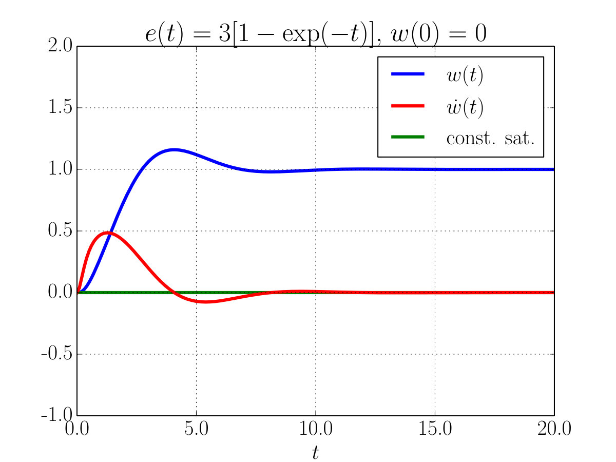 Figure 1
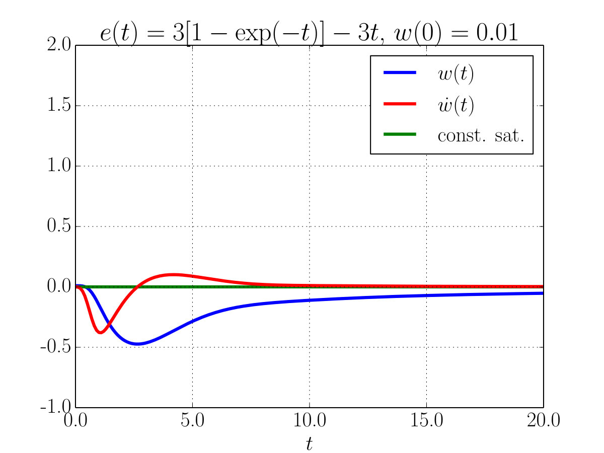 Figure 2
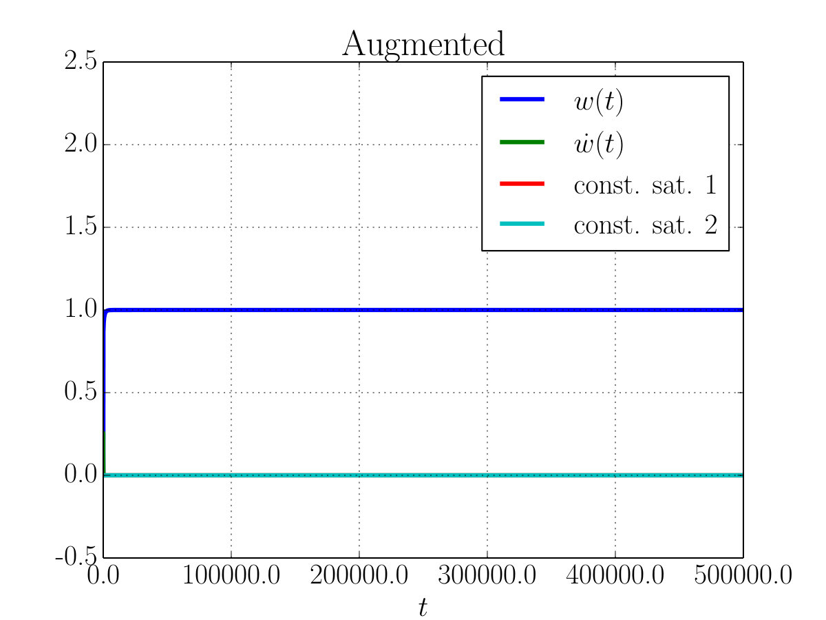 Figure 3
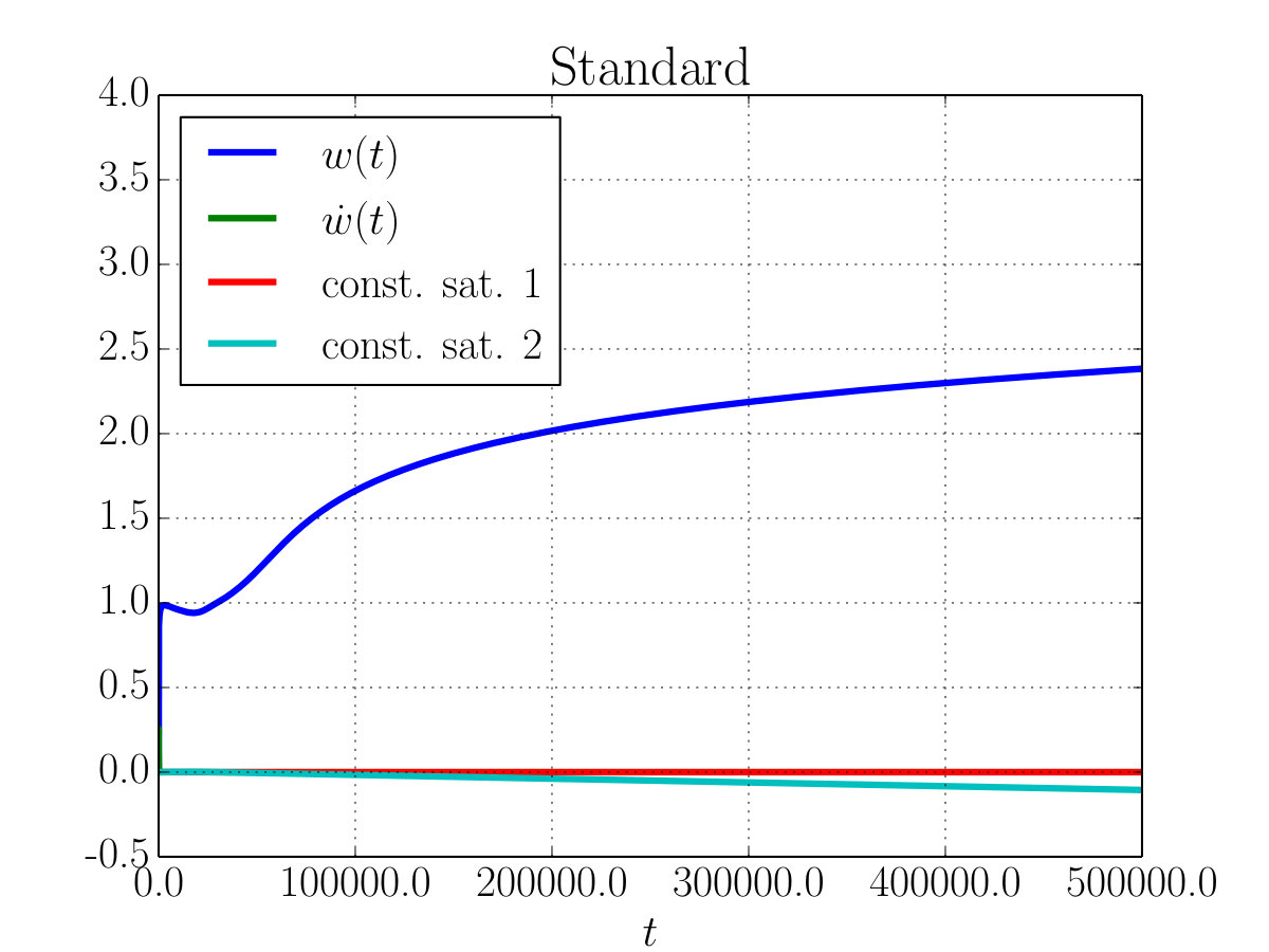 Figure 4
| Learning | Mechanics | Remarks |
|---|---|---|
| Weights and neuronal outputs are interpreted as generalized coordinates. | ||
| Weight variations and neuronal variations are interpreted as generalized velocities. | ||
| The cognitive action is the dual of the action in mechanics. |
Peer Reviews
No public reviews on file for this paper yet. If you reviewed it on a platform where reviews are public (OpenReview, ICLR, NeurIPS, ICML), you can paste yours below so the community can read it here.
Videos
No videos yet. Explain this paper in a talk, walkthrough, or lecture? Add one.
Taxonomy
TopicsNeural Networks and Applications · Model Reduction and Neural Networks · Neural dynamics and brain function
Spatiotemporal Local Propagation
Alessandro Betti
University of Florence
Florence, Italy
&Marco Gori
SAILab, University of Siena
Siena, Italy
Abstract
This paper proposes an in-depth re-thinking of neural computation that parallels apparently unrelated laws of physics, that are formulated in the variational framework of the least action principle. The theory holds for neural networks that are also based on any digraph, and the resulting computational scheme exhibits the intriguing property of being truly biologically plausible. The scheme, which is referred to as SpatioTemporal Local Propagation (STLP), is local in both space and time. Space locality comes from the expression of the network connections by an appropriate Lagrangian term, so as the corresponding computational scheme does not need the backpropagation (BP) of the error, while temporal locality is the outcome of the variational formulation of the problem. Overall, in addition to conquering the often invoked biological plausibility missed by BP, the locality in both space and time that arises from the proposed theory can neither be exhibited by Backpropagation Through Time (BPTT) nor by Real-Time Recurrent Learning (RTRL).
1 Introduction
Since mid-eighties, the explosion of interest in neural computation has been mostly fueled by finite-dimensional optimization in the space of the connection weights. Because of the typical large number of parameters involved, gradient-descent methods have dominated the searching heuristics. Moreover, it early became clear that large-scale problems can only be faced thanks to stochastic gradient descent (SGD) and related algorithms, that represent the on-line side of classic batch-mode optimization schemes. To some extent, SGD gives learning a sort of temporal dimension. If one assumes that the examples come at discrete time then weight updating takes place, for each example, at each temporal step. As early pointed out in the seminal PDP book (1) (p.324), on-line learning can be regarded as an approximation of gradient descent of the error function. In their words
By changing the weights after each pattern is presented we depart to some extent from a true gradient descent in . Nevertheless, provided the learning rate (i.e. the constant of proportionality) is sufficiently small, this departure will be negligible and the delta rule will implement a ver close approximation to gradient-descent in sum-squared error.
The resulting on-line process, along with mini-batch versions, have been the subject of in-depth recent investigations (e.g. (2)) that have contributed to shed light on SGD and on many specific versions that have been massively using in machine learning.
This paper is motivated by the curiosity of providing a truly new foundation of learning, where “time” is regarded as an intrinsic variable for the acquisition of concepts. Basically, we propose a formulation of learning by differential equations instead of by the dominating approach of using finite-dimensional optimization. This can be traced back to a number of relevant contributions, including (3) and (4), as well as to a recent interesting continuous-based formulation of deep learning (5). While following this track, this paper proposes a new view of learning, that can regarded as the outcome of laws of nature. We use the unifying view that arises from physics when using variational calculus and, particularly, when deriving laws of nature as stationary points of the action. We establish a parallel with mechanics according to which particle positions is associated with the neural parameters (weights and outputs), so as the velocity turns out to indicate the rate of the learning process (see Table 1). The kinetic energy has related meaning, while the potential energy indicates the degree of satisfaction of the environmental constraints – for instance, in case of supervised learning the potential turns out to be a loss function. Interestingly, the presence of motion constraints on particles has a counterpart in the constraints that express the neural model, so as “learning motion” is a stationary point of a functional, referred to as the cognitive action, under the neural architectural constraints. Like in mechanics, the resulting solution is a differential equations in the Lagrangian variables that dictates the evolution of the weights and of the neural outputs. The learning behavior reminds us of damped oscillators and the process of dissipation leads to ordered configurations which correspond to the outcome of learning. As dissipation increases the proposed theory leads to solutions that approaches classic gradient descent.
The most striking results of the theory are deeply rooted into the variational formulation under the subsidiary conditions, that represent the neural constraints. It is shown that STLP exhibits locality in both space and time for neural networks defined by any digraph. Temporal locality is basically the outcome of the variational optimization that yields models based on differential equation. Interestingly, space locality turns out to be the outcome of imposing the stationarity of the cognitive action under neural constraints. The issue of biological plausibility has been recently the subject of a related investigation in (6).
The message that emerges from the paper is that in order to gain a truly biological plausibility, temporal locality and strong space locality must be supported. On the other hand, classic algorithms for gradient computation in recurrent neural network do not exhibit this property: neither BPTT (BackPropation Through Time) nor Real-Time Recurrent Learning (RTRL) possess space and temporal locality. BPTT is local in space, but not in time, whereas RTRL is local in time, but not in space (7). Moreover, in these classic algorithms, space locality refers to the property gained by the backpropation factorization, not to strong space locality that is gained by STLP. Overall, the proposed theory stimulates a re-thinking of neural computation driven by laws of nature, where there is no distinction between learning and test, where the weight updating is paired with computation of the output in the learning environment. The theory also opens the doors for an in-depth reformulation of learning algorithms.
2 Modified Dirichlet problem
Let be an open, bounded domain in , let , and be, and define the following functional
[TABLE]
which is a weighted Dirichlet integral plus the term. We are here interested in the necessary conditions for to be an extremizer of the modified Dirichlet functional (1) subject to a class of holonomic constraints of the form 111In this section, for the sake of simplicity, we are considering holonomic constraints that do not depend explicitly on the independent variable , however the arguments presented here can be readily generalized also to include the case . Indeed in Section 3 we will consider general holonomic constraints. . Let us consider the problem in Eq. (1) where is subject to the constraints for all and of class . Furthermore assume that the Jacobian matrix defined by satisfies222We could ask for a less restrictive condition here, namely that should be full rank on all the points such that .:
[TABLE]
From the theory of calculus of variation with subsidiary conditions (see (8) Chap. 2) we know that there exist such that the constrained stationary points of coincides with the unconstrained stationary points of the extended functional
[TABLE]
and the Euler equation for this functional are 333throughout this paper we will adopt Einstein summation convention; that is to say two repeated indices, unless otherwise specified imply summation.
[TABLE]
where is the Euler operator ((8) p. 18 and (9)). Differentiating the constraints two times with respect to one obtaines
[TABLE]
Hence if we scalar multiply Euler equation by we obtain
[TABLE]
where we defined . Therefore Euler equations for the constrained functional (3) are (4) with
[TABLE]
Notice that in order to get from Eq. (6) to (7) we need to know that is invertible. Whenever our assumption (2) holds the Gram matrix turns out to be a invertible in view of the following (well known) lemma:
Lemma 1**.**
If ,…, are linear independent vectors, then the Gram matrix is positive definite.
Proof.
. However if and only if , therefore we can conclude that for every . ∎
3 Neural network constraints
The typical learning paradigm within the framework of NN consists of a model, that depends on a set of parameters , together with an update rule for the parameters; this rule is usually a gradient descent of a function that measure the goodness of the model on a specific learning task. However in this section we will show that when the dynamics of the parameters is described by laws that comes from stationarity conditions of a functional, as it happens for canonical coordinates in classical mechanics (see Table 1), then the NN model can be treated using the theory of constraints described in the previous sections. As an immediate consequence of this approach the learning process gains temporal and spatial locality even in the case of recurrent NN.
First of all let us describe the architecture of the models that we will address. Given a simple digraph of order without loss of generality we can assume and . A neural network constructed on consists of a set of maps444Please notice that now is a the variable of the variational problem, and therefore represent a mapping . It not to be intended as the independent variable of the problem described in the previous sections. and together with constraints where . Let be the set of all real matrices and the set of all strictly lower triangular matrices over . If we say that the NN has a feedforward structure. In this paper we will consider both feedforward NN and NN with cycles. The relations for specify the computational scheme with which the information diffuses trough the network. In a typical network with inputs these constraints are defined as follows (see also Fig. 1): For any vector , for any matrix with entries and for any given map we define the constraint on neuron when the example is presented to the network as
[TABLE]
where is of class .
Our goal here is to show that such relations, that normally are considered just a local description of the compositional structure of the NN, once properly interpreted as constraints in the space (see Fig. 1) are suitable holonomic subsidiary conditions in the sense of (2).
Like in the case of classical mechanics, when dealing with learning processes we are interested in the temporal dynamics of the variables when they are exposed to the data from which the learning is supposed to happen. For this reason in this section we can restrict ourselves to the case and regard this variable as time (). Moreover because the neural constraints involve not only but also the variables split into and .
Feedforward Networks. Now let us consider the case and let us extend the theory described in Eq. (1) by allowing , so that, in the end, we consider the functional
[TABLE]
subject to the constraints
[TABLE]
Then the following proposition holds true:
Proposition 1**.**
The matrix is full rank.
Proof.
First of all notice that if is full rank also has this property. Then, since
[TABLE]
we immediately notice that and that for all we have . This means that
[TABLE]
which is clearly full rank. ∎
Notice that this result heavily depends on the assumption ; however we will now discuss how the introduction of an additional variable that models the degree of satisfaction of the neural constraints acts as a regularizer of constraints (8) and ensure the satisfaction of (2).
Recurrent networks. Let us suppose that we also assign to each neuron a variable that measure the degree of violation of the constraint. Then Eq. (10) assumes the form , where
[TABLE]
In doing so it is important to notice that Proposition 1 holds without the assumption that as it is immediate to prove since , which is of course full rank. This important remark opens the possibility to extend the theory to networks with “feedback” connections based on general simple digraphs.
In this formulation of the theory the action, described in Eq. (9) must be modified to take into account of the introduction of the new variable :
[TABLE]
where .
4 Cognitive action and laws of learning: Feedforward architecture
In the previous section we concentrated ourselves on showing that the set of constraints that define a NN are good constraints (in the sense of (2)). In this section we will focus on the feedforward case described by the functional (9) together with constraints (10). In particular we will discuss the updates rules (Euler-Lagrange equations) for the variables and derived from the stationarity conditions of the functional (9). We notice in passing that when imposing the stationarity of action we give rise to a computational model that, in general, is remarkably different from classic optimization approaches used in machine learning, that are typically driven by the gradient heuristics. Basically, the models arising from , instead of gradually reducing the action from its initial value, satisfy this condition for any time instant, thus resembling what happens for Newtonian’s laws.
We begin by deriving the constrained Euler-Lagrange (EL) equations associated with the functional (9) under subsidiary conditions (10). The constrained functional is
[TABLE]
and its EL-equations thus read
[TABLE]
where , are the functional derivatives of with respect to and respectively (see (9)). An expression for Lagrange multiplies, as it is explained in Section 2 is derived by differentiating two times the constraint with respect to the time and using the obtained expression to substitute the second order terms in the Euler equations. In this case the analogue of Eq. (6) is
[TABLE]
where , , , , and are the gradients and the hessians of constraint (10).
**Initial conditions. ** Suppose now that we want to solve Eq. (14)–(15) with Cauchy initial conditions. Of course we must choose and such that , where we posed , for . However since the constraint must hold also for all we must also have at least . These conditions written explicitly means
[TABLE]
If the constraints does not depend explicitly on time it is sufficient to to choose and , while for time dependent constraint this condition leaves
[TABLE]
which is an additional constraint on the initial conditions and to be satisfied. Therefore one possible consistent way to impose Cauchy conditions is
[TABLE]
Higher derivative of becomes automatically satisfied thanks through the differential equations.
Supervised Learning and reduction to BP. In order to see how this theory can be readily applied to learning let us restrict ourselves to the case and choose , , . Now let us choose
[TABLE]
where is an assigned supervision signal and
[TABLE]
being the variables associated with the outputs neurons. A typical input signal and the corresponding supervision signal can be constructed from a standard training set in the following manner. Choose a sequence of times such that is constant . Furthermore define the following sequences: and . Let , where are standard Friedrichs mollifiers and define
[TABLE]
where is the characteristic function of the set and . Then the signal
[TABLE]
is piecewise constant signals with smooth transitions. The temporal behaviour of these signals is depicted in the side figure.
To understand the behaviour of the Euler equations (14) and (15) we observe that in the case of feedforward networks, as it is well known, the constraints can be solved for so that eventually we can express the value of the output neurons in terms of the value of the input neurons. If we let be the value of when , then the theory defined by (9) under subsidiary conditions (10) is equivalent, when , to the unconstrained theory defined by
[TABLE]
where . The Euler equations associated with (18) are
[TABLE]
that in the limit and reduces to the gradient method
[TABLE]
with learning rate . Notice that the presence of the term that we proposed in the general theory it is essential in order to have a learning behaviour as it produce dissipation.
Typically the term in Eq. (20) can be evaluated using the Backpropagation algorithm; we will now show that Eq. (14)–(16) in the same limit used above , , reproduces Eq. (20) where the term explicitly assumes the form prescribed by BP. In order to see this choose and multiply both sides of Eq. (14)–(16) by , then take the limit , , . In this limit Eq. (15) and Eq. (16) becomes respectively
[TABLE]
where is the limit of . Because the matrix not only is invertible, but it is a Gram matrix if we define , then we have . If we then pose , the ’s satisfies with that is an upper triangular matrix. Solving this equation is equivalent to the solution of and . From this last equation we immediately see that once is known is recursively derived starting from the output neurons. Finally, we can interpret in Eq. (22) as the delta-error, which is the recursively determined by Eq. (21) because of the special structure of of matrix .
Optimal inversion of . Since is Gram matrix, its inversion of , which is required for determining in Eq. 16, can be efficiently determined with an optimal complexity (10). Basically, we only need a number of dominant floating-point operation with grows quadratically with the dimension of .
4.1 Simulation of the dynamics
In order to prove the soundness of the proposed theory we performed some simulations of the Euler equations (14) and (15) in the special case , , and , where in particular is taken to be a quadratic loss on the output neuron. To understand the learning dynamic of the weights we choose a constant supervision signal and various time-dependent input signals . Figure 2 shows the evolution of the weight of a single linear neuron with a target and a variable input . In Fig. 2–(a) as , and indeed converges to . In Fig. 2–(b) and consistently . Notice that in both cases the neuron constraint is always exactly satisfied. Remember that the initial conditions must be consistent with Eq. (17); in this example in Fig. 2–(a) we have that guaranteed , while in the experiment relative to Fig. 2–(b) one can choose as the condition is ensured by .
In Fig. 3 instead we tested the robustness of the method with respect to numerical errors by running the simulation for a longer period of time. The model here consists of two neurons NN with nonlinear activation function. We observed that due to numerical errors the system can fail to converge to the correct solution (Fig. 3–(a)). This can be understood as soon as we realize that, following the ideas of Section 2, EL-equations implements only the satisfaction of the second derivative of the constraints, therefore errors on the trajectories can shift the dynamic of the system on another constraint that differs from the correct one by a linear function of time. Hence, we found that such behaviour can be effectively corrected (see Fig. 3–(b)) by adding to the potential a quadratic loss on the constraint itself.
5 Conclusions
This paper proposes a novel formulation of learning by differential equations instead of by the dominating approach of using finite-dimensional optimization. This can be traced back many contributions that early appeared at the of the eighties (see e.g. (3) and (4)), as well as from the recent trend of emphasizing continuous-based computational models of learning (see e.g. (5)555Best student paper awards at NeurIPS 2018.. The distinctive view proposed in this paper consists of the close parallel with mechanics, that arises from the general principle of formulating variational laws of nature. The STLP computational scheme possesses the distinctive feature of being local in both space and time. Moreover, the gained space locality property goes beyond the classic local neural communication required for computing the gradient. Unlike BP, there is no need to synchronize the forward and backward step that return the factors of the gradient, since they are locally available. The theory nicely addresses classic arguments on BP biologically plausibility (11), and opens the doors to an in-depth reformulation of learning algorithms for both feedforward and recurrent neural networks.
The reference list from the paper itself. Each links out to its DOI / PubMed record.
- 1(1) D.E. Rumelhart, J.L. Mc Clelland, and the PDP Research Group. Parallel Distributed Processing: Explorations in the Microstructure of Cognition , volume 1. MIT Press, Cambridge, 1986.
- 2(2) Léon Bottou, Frank E. Curtis, and Jorge Nocedal. Optimization methods for large-scale machine learning. SIAM Review , 60(2):223–311, 2018.
- 3(3) F.J. Pineda. Generalization of back-propagation to recurrent neural networks. Physical Review Letters , 59:2229–2232, 1987.
- 4(4) B.A. Pearlmutter. Learning state space trajectories in recurrent neural networks. Neural Computation , 1:263–269, 1989.
- 5(5) Tian Qi Chen, Yulia Rubanova, Jesse Bettencourt, and David K. Duvenaud. Neural ordinary differential equations. In Samy Bengio, Hanna M. Wallach, Hugo Larochelle, Kristen Grauman, Nicolò Cesa-Bianchi, and Roman Garnett, editors, Neur IPS , pages 6572–6583, 2018.
- 6(6) Yoshua Bengio, Dong-Hyun Lee, Jörg Bornschein, and Zhouhan Lin. Towards biologically plausible deep learning. Co RR , abs/1502.04156, 2015.
- 7(7) R.J. Williams and D. Zipser. A learning algorithm for continually running fully recurrent neural networks. Neural Computation , 1:270–280, 1989.
- 8(8) Mariano Giaquinta and Stefan Hildebrandt. Calculus of variations, vol. i. number 310 in a series of comprehensive studies in mathematics, 1996.